Synchronization in networks of networks: The onset of coherent collective behavior in systems of interacting populations of heterogeneous oscillators

Abstract

The onset of synchronization in networks of networks is investigated. Specifically, we consider networks of interacting phase oscillators in which the set of oscillators is composed of several distinct populations. The oscillators in a given population are heterogeneous in that their natural frequencies are drawn from a given distribution, and each population has its own such distribution. The coupling among the oscillators is global, however, we permit the coupling strengths between the members of different populations to be separately specified. We determine the critical condition for the onset of coherent collective behavior, and develop the illustrative case in which the oscillator frequencies are drawn from a set of (possibly different) Cauchy-Lorentz distributions. One motivation is drawn from neurobiology, in which the collective dynamics of several interacting populations of oscillators (such as excitatory and inhibitory neurons and glia) are of interest.

In recent years, there has been considerable interest in networks of interacting systems. Researchers have found that an appropriate description of such systems involves an understanding of both the dynamics of the individual oscillators and the connection topology of the network. Investigators studying the latter have found that many complex networks have a modular structure involving motifs [1], communities [2, 3], layers [4], or clusters [5]. For example, recent work has shown that as many kinds of networks (including isotropic homogeneous networks and a class of scale-free networks) transition to full synchronization, they pass through epochs in which well-defined synchronized communities appear and interact with one another [3]. Knowledge of this structure, and the dynamical behavior it supports, informs our understanding of biological [6], social [7], and technological networks [8].

Here we consider the onset of coherent collective behavior in similarly structured systems for which the dynamics of the individual oscillators is simple. In seminal work, Kuramoto analyzed a mathematical model that illuminates the mechanisms by which synchronization arises in a large set of globally-coupled phase oscillators [9]. An important feature of Kuramoto’s model is that the oscillators are heterogeneous in their frequencies. And, although these mathematical results assume global coupling, they have been fruitfully applied to further our understanding of systems of fireflies, arrays of Josephson junctions, electrochemical oscillators, and many other cases [10].

In this work, we study systems of several interacting Kuramoto systems, i.e., networks of interacting populations of phase oscillators. Our motivation is drawn not only from the applications listed above (e.g., an amusing application might be interacting populations of fireflies, where each population inhabits a separate tree), but also from other biological systems. Rhythms arising from coupled cell populations are seen in many of the body’s organs (including the heart, the pancreas, and the kidneys, to name but a few), all of which interact. For example, the circadian rhythm influences many of these systems. We draw additional motivation from consideration of how neuronal tissue is organized. Although we do not consider neuronal systems specifically in this paper, we note that heterogeneous ensembles of neurons often exhibit a “network-of-networks” topology. At the cellular level, populations of particular kinds of neurons (e.g., excitatory neurons) interact not only among themselves, but also with populations of other distinct neuronal types (e.g., inhibitory neurons). At a higher level of organization, various anatomical regions of the brain interact with one another as well [6].

Although our network is simple, it is novel in that we include heterogeneity at several levels. Each population consists of a collection of phase oscillators whose natural frequencies are drawn at random from a given distribution. To allow for heterogenity at the population level, we let each population have its own such frequency distribution. In addition, our system is heterogeneous at the coupling level as well: we consider global coupling such that the coupling strengths between the members of different populations can be separately specified.

The assumpion of global (but population-weighted) coupling permits an analytic determination of the critical condition for the onset of coherent collective behavior, as we will show. While this assumption may not strictly apply in some applications, our results provide insight into the behavior of networks of similar topology even if the connectivity is less than global.

We begin by specifying our model and deriving our main results. We then discuss several illustrative examples.

Consider first a two-species Kuramoto model. We label the separate species θ and φ and assume that there are N_θ and N_φ such oscillators in each population, respectively. Thus, the system equations are

$$\begin{array}{l}\frac{d{\theta }_i}{dt}={\omega }_{\theta i}+\eta \frac{k_{\theta \theta }}{N_{\theta }}\sum _{j=1}^{N_{\theta }}\mathit{sin}({\theta }_j-{\theta }_i-{\alpha }_{\theta \theta })+\eta \frac{k_{\theta \phi }}{N_{\phi }}\sum _{j=1}^{N_{\phi }}\mathit{sin}({\phi }_j-{\theta }_i-{\alpha }_{\theta \phi }),\\ \frac{d{\phi }_i}{dt}={\omega }_{\phi i}+\eta \frac{k_{\phi \theta }}{N_{\theta }}\sum _{j=1}^{N_{\theta }}\mathit{sin}({\theta }_j-{\phi }_i-{\alpha }_{\phi \theta })+\eta \frac{k_{\phi \phi }}{N_{\phi }}\sum _{j=1}^{N_{\phi }}\mathit{sin}({\phi }_j-{\phi }_i-{\alpha }_{\phi \phi }).\end{array}$$

Here, η is an overall coupling strength, the α’s provide additional heterogeneity in the coupling functions, and the matrix

$$\mathbf{K}=\left(\begin{array}{ll}{k}_{\theta \theta }\hfill & k_{\theta \phi }\hfill \\ k_{\phi \theta }\hfill & k_{\phi \phi }\hfill \end{array}\right)$$ (1)

defines the connectivity among the populations [11].

For arbitrarily many different species, let σ range over the various population symbols θ, φ, … with the understanding that depending on the context, σ may represent either a label (when subscripted) or a variable. Thus, we have

$$\frac{d{\sigma }_i}{dt}={\omega }_{\sigma i}+\sum _{{\sigma }^{\prime }}\left[\eta \frac{k_{\sigma {\sigma }^{\prime }}}{N_{{\sigma }^{\prime }}}\sum _{j=1}^{N_{{\sigma }^{\prime }}}\mathit{sin}({\sigma }_j^{\prime }-{\sigma }_i-{\alpha }_{\sigma {\sigma }^{\prime }})\right].$$

The ω_σi are the constant natural frequencies of the oscillators when uncoupled, and are distributed according to a set of time-independent distribution functions G_σ(ω_σ) [12].

We define the usual Kuramoto order parameter for each population, i.e.,

$$r_{\sigma }{e}^{i{\psi }_{\sigma }}=\frac{1}{N_{\sigma }}\sum _{j=1}^{N_{\sigma }}{e}^{i{\sigma }_j}.$$

Here, r_σ describes the degree of synchronization in each population, and ranges from 0 to 1. Using this, the above equations can be expressed

$$\frac{d{\sigma }_i}{dt}={\omega }_{\sigma i}+\sum _{{\sigma }^{\prime }}\eta k_{\sigma {\sigma }^{\prime }}{r}_{{\sigma }^{\prime }}\mathit{sin}({\psi }_{{\sigma }^{\prime }}-{\sigma }_i-{\alpha }_{\sigma {\sigma }^{\prime }}).$$

Assuming that the N_σ are very large, we solve for the onset of coherent collective behavior by using a distribution function approach. Thus, instead of discrete indicies, we imagine continua of oscillators described by distribution functions F_σ(σ, ω_σ, t) such that F_σ(σ, ω_σ, t)dσdω_σ is the fraction of σ-oscillators whose phases and natural frequencies lie in the infinitesimal volume element dσdω_σ at time t. Note that in the N_σ → ∞ limit,

$$G_{\sigma }({\omega }_{\sigma })={\int }_0^{2\pi }{F}_{\sigma }(\sigma ,{\omega }_{\sigma },t)d\sigma ,$$

and the order parameters are given by

$$r_{\sigma }{e}^{i{\psi }_{\sigma }}=\iint F_{\sigma }{e}^{i\sigma }d\sigma d{\omega }_{\sigma }.$$ (2)

In this context, the distribution functions satisfy the equations of continuity, i.e.,

$$\frac{\partial F_{\sigma }}{\partial t}+\overrightarrow{\nabla }·(F_{\sigma }\frac{d\sigma }{dt}\widehat{\sigma })=0,$$

and if we write F_σ(σ, ω_σ, t) = f_σ(σ, ω_σ, t)G_σ(ω_σ), we have

$$\frac{\partial f_{\sigma }}{\partial t}+\frac{\partial }{\partial \sigma }\left\{\left[{\omega }_{\sigma }+\sum _{{\sigma }^{\prime }}\eta k_{\sigma {\sigma }^{\prime }}{r}_{{\sigma }^{\prime }}\mathit{sin}({\psi }_{{\sigma }^{\prime }}-\sigma -{\alpha }_{\sigma {\sigma }^{\prime }})\right]f_{\sigma }\right\}=0.$$ (3)

The incoherent state has σ distributed uniformly over [0, 2π], so that f_σ = 1/2π and r_σ = 0. These satisfy Eq. (3) trivially. We test the stability of this solution by perturbing it. Note that a perturbation to f_σ leads to a perturbation of r_σ, and we expect these perturbations to either grow or shrink exponentially in time, depending on the overall coupling strength η. The marginally stable case occurs at a critical value η* at which coherent collective behavior emerges.

Thus, we write f_σ = 1/2π + (δf_σ)e^st and r_σ = (δr_σ)e^st, where (δf_σ) and (δr_σ) are small. Inserting the first of these into the continuity equation (Eq. (3)), and keeping only first-order terms, we obtain

$$s(\delta f_{\sigma })+{\omega }_{\sigma }\frac{\partial }{\partial \sigma }(\delta f_{\sigma })=\frac{1}{2\pi }\sum _{{\sigma }^{\prime }}\eta k_{\sigma {\sigma }^{\prime }}(\delta r_{{\sigma }^{\prime }})cos({\psi }_{{\sigma }^{\prime }}-\sigma -{\alpha }_{\sigma {\sigma }^{\prime }}).$$

The solution to this equation is

$$(\delta f_{\sigma })=\frac{1}{4\pi }\sum _{{\sigma }^{\prime }}\eta k_{\sigma {\sigma }^{\prime }}(\delta r_{{\sigma }^{\prime }})\left[\frac{e^{i({\psi }_{{\sigma }^{\prime }}-\sigma -{\alpha }_{\sigma {\sigma }^{\prime }})}}{s-i{\omega }_{\sigma }}+\frac{e^{-i({\psi }_{{\sigma }^{\prime }}-\sigma -{\alpha }_{\sigma {\sigma }^{\prime }})}}{s+i{\omega }_{\sigma }}\right].$$ (4)

Consistency demands that the perturbations (δf_σ) and (δr_σ) be related to each other via the order parameter equation, Eq. (2). This yields our main result, as follows. Eq. (2) becomes

$$(\delta r_{\sigma })e^{st}{e}^{i{\psi }_{\sigma }}={\int }_{-\infty }^{\infty }{G}_{\sigma }({\omega }_{\sigma }){\int }_0^{2\pi }\left(\frac{1}{2\pi }+(\delta f_{\sigma })e^{st}\right)e^{i\sigma }d\sigma d{\omega }_{\sigma }.$$

The integral involving 1/2π is zero. Inserting the solution for (δf_σ) from Eq. (4), one obtains [13]

$$(\delta r_{\sigma })e^{i{\psi }_{\sigma }}=\left[\frac{1}{2}{\int }_{-\infty }^{\infty }\frac{G_{\sigma }({\omega }_{\sigma })}{s-i{\omega }_{\sigma }}d{\omega }_{\sigma }\right]\sum _{{\sigma }^{\prime }}\eta k_{\sigma {\sigma }^{\prime }}(\delta r_{{\sigma }^{\prime }})e^{i({\psi }_{{\sigma }^{\prime }}-{\alpha }_{\sigma {\sigma }^{\prime }})}.$$

Define the bracketed expression to be g_σ(s), and define z_σ = (δr_σ)e^iψ_σ. Then, we have

$$z_{\sigma }=g_{\sigma }(s)\sum _{{\sigma }^{\prime }}\eta k_{\sigma {\sigma }^{\prime }}{e}^{-i{\alpha }_{\sigma {\sigma }^{\prime }}}{z}_{{\sigma }^{\prime }}.$$

Now define the complex quantity k̄_σσ′ = ηk_σσ′e^{−iα_σσ′}. Using the Kronecker delta δ_σσ′, the above equation can be written

$$\sum _{{\sigma }^{\prime }}\left({\overline{k}}_{\sigma {\sigma }^{\prime }}-\frac{{\delta }_{\sigma {\sigma }^{\prime }}}{g_{\sigma }(s)}\right)z_{{\sigma }^{\prime }}=0.$$

In matrix notation for the case of two populations labeled θ and φ, this is

$$\left(\begin{array}{cc}{\overline{k}}_{\theta \theta }-\frac{1}{g_{\theta }(s)}& {\overline{k}}_{\theta \phi }\\ {\overline{k}}_{\phi \theta }& {\overline{k}}_{\phi \phi }-\frac{1}{g_{\phi }(s)}\end{array}\right)\left(\begin{array}{c}{z}_{\theta }\\ z_{\phi }\end{array}\right)=0.$$ (5)

This equation has a non-trivial solution if the determinant of the matrix is zero. This condition determines the growth rate s in terms of η, k̄_σσ′, and the parameters of the distributions G_σ(ω_σ) (via g_σ(s)).

To illustrate the resulting behavior, we note that g_σ(s) can be evaluated in closed form for a Cauchy-Lorentz distribution

$$G_{\sigma }({\omega }_{\sigma })=\frac{{\mathrm{\Delta }}_{\sigma }}{\pi }·\frac{1}{{({\omega }_{\sigma }-{\mathrm{\Omega }}_{\sigma })}^2+{\mathrm{\Delta }}_{\sigma }^2},$$ (6)

where Ω_σ, the mean frequency of population σ, and the half-width-at-half-maximum Δ_σ are both real, and Δ_σ is positive. One obtains

$$\frac{1}{g_{\sigma }({\omega }_{\sigma })}=2(s+{\mathrm{\Delta }}_{\sigma }+i{\mathrm{\Omega }}_{\sigma }).$$

Using this, the determinant condition for the two-population case reduces to

$$[{\overline{k}}_{\theta \theta }-2(s+{\mathrm{\Delta }}_{\theta }+i{\mathrm{\Omega }}_{\theta })][{\overline{k}}_{\phi \phi }-2(s+{\mathrm{\Delta }}_{\phi }+i{\mathrm{\Omega }}_{\phi })]-{\overline{k}}_{\theta \phi }{\overline{k}}_{\phi \theta }=0.$$

For simplicity, we set the phase angles α_σσ′ to zero for the remainder of this paper [14]. In this case, the matrix elements k̄_σσ′ are purely real, so that k̄_σσ′ = ηk_σσ′. The determinant condition then becomes

$$[\eta k_{\theta \theta }-2(s+{\mathrm{\Delta }}_{\theta }+i{\mathrm{\Omega }}_{\theta })][\eta k_{\phi \phi }-2(s+{\mathrm{\Delta }}_{\phi }+i{\mathrm{\Omega }}_{\phi })]-{\eta }^2{k}_{\theta \phi }{k}_{\phi \theta }=0.$$ (7)

Notice that if η = 0, then s = −Δ_σ − iΩ_σ, indicating that the incoherent state is stable for zero coupling (since −Δ_σ is negative). We imagine increasing (or decreasing) η until s crosses the imaginary axis at a critical value η*. At this point, the incoherent state loses stability and coherent collective behavior emerges in the ensemble. Thus, the critical value η* can be determined from the determinant condition by setting s = iυ, where υ is real (so that the perturbations are marginally stable), and equating the real and imaginary parts of the left side of Eq. (7) to zero. This results in two equations which can be solved simultaneously for the two (real) unknowns η and υ.

For our first example, we choose two identical populations; we set Δ_θ = Δ_φ = Δ and Ω_θ = Ω_φ = Ω. (A more generic example will follow.) Denoting D = det(K) and T = tr(K), we separate the real and imaginary parts of Eq. (7) to obtain

$$\begin{array}{c}D{\eta }^2-2\mathrm{\Delta }T\eta +4{\mathrm{\Delta }}^2-4{(v+\mathrm{\Omega })}^2=0\\ (v+\mathrm{\Omega })(4\mathrm{\Delta }-\eta T)=0.\end{array}$$ (8)

One solution to these equations is

$$v_{\ast }=-\mathrm{\Omega },{\eta }_{\ast }=\mathrm{\Delta }\left(\frac{T\pm \sqrt{T^2-4D}}{D}\right),$$

which is valid for T² ≥ 4D, since η is assumed to be real. Notice that the appropriate solution as D → 0 (using the negative sign for T > 0 and the positive sign for T < 0) is

$$v_{\ast }=-\mathrm{\Omega },{\eta }_{\ast }=\frac{2\mathrm{\Delta }}{T},$$

as can be verified by setting D = 0 in Eq. (8) directly. Another solution is

$$v_{\ast }=-\mathrm{\Omega }\pm \frac{\mathrm{\Delta }}{T}\sqrt{4D-T^2},{\eta }_{\ast }=\frac{4\mathrm{\Delta }}{T}.$$

Finally, setting T = 0 in Eq. (8) yields υ* = −Ω and ${\eta }_{\ast }=\pm \frac{2\mathrm{\Delta }}{\sqrt{-D}}$ for D < 0, and no solution for D ≥ 0. These results are summarized in Table I.

TABLE I.

Solutions to Eq. (8) for two identical populations. D = det(K) and T = tr(K), where K is the connectivity matrix (Eq. (1)), and Δ is the width parameter in Eq. (6).

Case	Condition	υ*	η *
1	T2 > 4D	−Ω	$\mathrm{\Delta }\left(\frac{T\pm \sqrt{T^2-4D}}{D}\right)$
2	T2 ≤ 4D	$-\mathrm{\Omega }\pm \frac{\mathrm{\Delta }}{T}\sqrt{4D-T^2}$	$\frac{4\mathrm{\Delta }}{T}$
3	D = 0	−Ω	$\frac{2\mathrm{\Delta }}{T}$
4	T = 0, D < 0	−Ω	$\pm \frac{2\mathrm{\Delta }}{\sqrt{-D}}$
5	T = 0, D ≥ 0	no solution	no solution

Thus, the critical values η* are determined by T, D, and Δ. To illustrate this result, we begin by discussing a particular example. Consider the matrix

$$\mathbf{K}=\left(\begin{array}{cc}1& -1\\ 1& 0\end{array}\right),$$

which has trace T = 1 and determinant D = 1. This corresponds to case two in Table I, from which we find that η* = 4Δ/T. Fig. 1 shows the results of a numerical simulation of two populations of 10, 000 oscillators each, using Δ = 1. The order parameters r_σ versus η are shown, and we can see that the oscillator populations are incoherent for η values below the predicted critical value η* = 4, and that they grow increasingly synchronized as η is increased beyond η*.

FIG. 1.

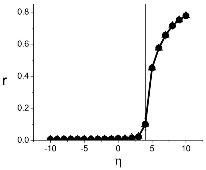
Numerical calculation of the order parameters (●, △) versus η for case A in Table II. The vertical line corresponds to the predicted value η* = 4. The data point nearest η* is at η = 4.15.

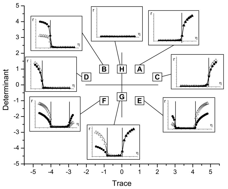
Next, we examined eight different connectivity matricies K that were chosen to sample the various regions in T − D space. Table (II) shows these matricies and the corresponding value(s) of η*. These predictions were tested by numerically calculating the order parameters r_σ for a range of coupling values η [15]. Results are shown in Fig. 2. The various cases are located by letter in the D − T plane according to the trace and determinant of the matricies, and the corresponding inset shows the numerically-calculated order parameters plotted versus η, with the predicted critical coupling indicated by a vertical line at η = η*. For example, the inset to case A (with (T, D) = (1, 1)) corresponds to Fig. 1, which was discussed above. It can be seen that for all cases, the onset of synchronization occurs as predicted.

FIG. 2.

Numerical simulations using the matricies listed in Table (II) for identical populations. The letters indicate the placement of each case in the T − D plane, and the corresponding insets show numerical calculations of the order parameters (●, △) versus η for that case (in all cases, η = 0 is in the center of the horizontal axis). Vertical lines in the insets indicate the predicted value(s) η* listed in Table (II) for the onset of coherent collective behavior. In all cases, we used Δ = 1. Note that for D > 0, there is one value of η*, whose sign corresponds to the sign of the trace T. If D ≥ 0 and T = 0, then synchronization is not possible for any coupling strength. For D < 0, there are two values of η*: one positive, and one negative.

Note that more than one prediction for η* may be specified by our analysis (see Table I). The solutions closest to η = 0 are the relevant ones, because we expect the incoherent state to lose stability once the first η* solution is encountered. There are two possible cases depending on the sign of D. First, if the two solutions have the same sign, then there is only one critical value η* (which may be positive or negative depending on the sign of the trace) for the onset of synchronization. This occurs for D > 0 and T ≠ 0, as can be seen in Fig. 2. (Interestingly, for D > 0 and T = 0, synchronization does not occur for any η.) The other case occurs for D < 0, for which the two η* solutions have opposite signs. In this case, there are two critical values η* for the onset of synchronization – one on either side of η= 0. This can also be observed in Fig. 2.

In the more general case in which the various populations have different natural frequency distributions, it is not typically possible to describe the onset of synchronization in terms of the determinant and trace of the coupling matrix K = k_σσ′ alone. We now consider this situation, but retain the Cauchy-Lorentz form of the natural frequency distributions for convenience. We manipulate Eq. (7) as follows. Let s = iυ (i.e., purely imaginary, to consider the marginally stable case) and define a = Δ_θ + i(υ + Ω_θ) and b = Δ_φ + i(υ + Ω_φ). We obtain

$$D{\eta }^2-2\eta (b{k}_{\theta \theta }+a{k}_{\phi \phi })+4ab=0.$$ (9)

There are two unknowns in this equation: η and υ. Eq. (9) is a quadratic equation in η with complex coefficients, and we can easily obtain two complex solutions η^(1,2) as functions of υ. Since the critical values ${\eta }_{\ast }^{(1,2)}$ must be real, we solve for the roots of Im(η^(1,2)), and evaluate Re(η^(1,2)) at these roots. This yields the possible critical values ${\eta }_{\ast }^{(1,2)}$. Typically, these steps must be performed symbolically and/or numerically; we used MATLAB^® [16]. As before, the values of ${\eta }_{\ast }^{(1,2)}$ that are closest to zero (on either side) are the relevant values.

To illustrate, we choose two populations with Cauchy-Lorentz natural frequency distributions (Eq. (6)) with parameters Δ_θ = 1, Ω_θ = 2, Δ_φ = 0.5, and Ω_φ = 4. We consider the same K matricies as before, i.e., those listed in the second column of Table II. Case E is straightforward; the analysis is illustrated in Fig. (3) and the numerical verification is in Fig. (4). Note that since Eq. (9) has complex coefficients, obtaining η typically involves taking the square root of a complex number. Therefore, one must be mindful of branch cuts when obtaining symbolic and/or numerical solutions. This is important in the analysis for case A, shown in Figs. (5) and (6). Finally, case H, which exhibits no synchronization for identical populations for any value of η, does show synchronization in the present case. The analysis is shown in Figs. (7–8).

TABLE II.

Connectivity matricies K chosen to sample T − D space.

Case	Matrix	T	D	η*
A	$\left(\begin{array}{cc}1& -1\\ 1& 0\end{array}\right)$	1	1	4
B	$\left(\begin{array}{cc}-2& -3\\ 1& 1\end{array}\right)$	−1	1	−4
C	$\left(\begin{array}{cc}3& 1\\ -3.5& -1\end{array}\right)$	2	0.5	$2(2-\sqrt{2})=1.172$
D	$\left(\begin{array}{cc}-3& 1\\ -3.5& 1\end{array}\right)$	−2	0.5	$2(-2+\sqrt{2})=-1.172$
E	$\left(\begin{array}{cc}-1& -1\\ 1& 2\end{array}\right)$	1	−1	$-(1\pm \sqrt{5})=-3.236,1.236$
F	$\left(\begin{array}{cc}1& 1\\ -1& -2\end{array}\right)$	−1	−1	$1\pm \sqrt{5}=-1.236,3.236$
G	$\left(\begin{array}{cc}2& 1\\ -3& -2\end{array}\right)$	0	−1	±2
H	$\left(\begin{array}{cc}1& -1\\ 2& -1\end{array}\right)$	0	1	None

FIG. 3.

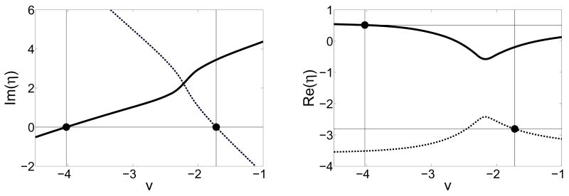
Case E, different populations. The left panel shows Im(η^(1,2)), with the vertical lines identifying roots at υ₁ = −4.024 and υ₂ = −1.722. The right panel shows Re(η^(1,2)); values at the roots found above are indicated by horizontal lines, yielding ${\eta }_{\ast }^{(1)}=0.515$ and ${\eta }_{\ast }^{(2)}=-2.809$. Thus, we expect synchronization to occur at these values as η is either increased or decreased away from zero.

FIG. 4.

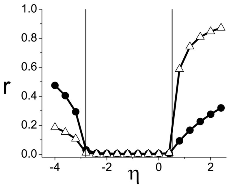
Case E, different populations. Calculations of the order parameters versus η confirm that the onset of synchronization occurs at η* = −2.809 and 0.515 (vertical lines), as predicted in Fig. (3).

FIG. 5.

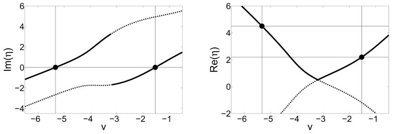
Case A, different populations. Panels as in Fig. (3). Note that the standard branch cut leads to discontinutites and the occurrence of two roots for Im(η⁽¹⁾)(υ) (solid lines, left panel), and none for Im(η⁽²⁾)(υ) (dotted lines, left panel). From the right panel we find η* = 2.189, 4.501, taking care to obtain these from Re(η⁽¹⁾) (solid line, right panel). We expect to find synchronization onset at the smaller of these values.

FIG. 6.

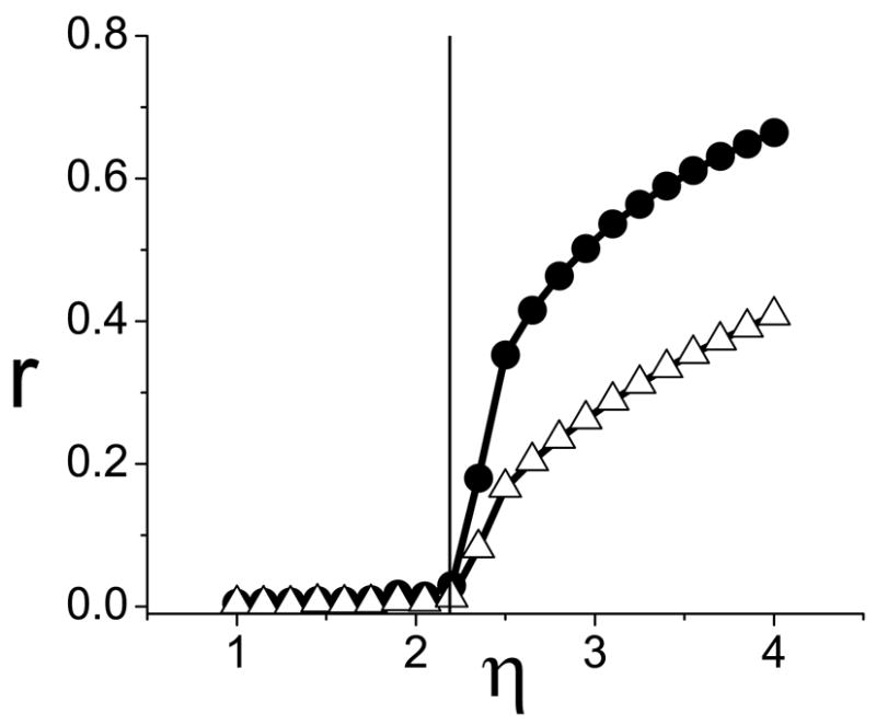
Case A, different populations: The onset of synchronziation occurs at η* = 2.189 (vertical line), as predicted in Fig. (5). No synchronization is observed for smaller values of η (not shown).

FIG. 7.

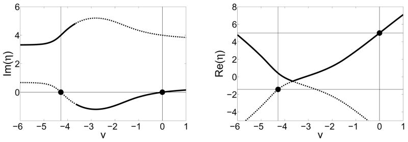
Case H, different populations. We find η* = −1.429, 5.000.

FIG. 8.

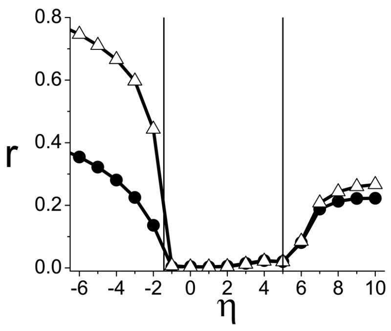
Case H, different populations. Synchronization occurs at η* = −1.429 and 5.000 (vertical lines), as predicted in Fig. (7).

We close by giving an example with three different populations. We choose the same Cauchy-Lorentz distributions as above, and add a third with Δ_ρ = 1/3 and Ω_ρ = 1. We use the following K matrix:

$$\left(\begin{array}{ccc}-1& 1& 1\\ 1& -1& 1\\ 1& 1& -1\end{array}\right).$$

The procedure for deriving η* proceeds as above, except that Eq. (7) is replaced by a third-degree polynomial in η. Fig. (9) shows the imaginary and real parts of the three η solutions. (Note that the branch cuts are more complicated.) The predicted onset of synchronization was verified, as shown in Fig. (10).

FIG. 9.

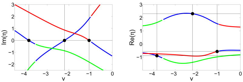
(Color online) Three populations. The imaginary and real parts of η^(1,2,3) are plotted in blue, red, and green to illustrate the discontinuties due to branch cuts. The analysis proceeds as in the previous cases. Because of branch cuts, two roots occur on η⁽¹⁾, one on η⁽²⁾, and none on η⁽³⁾. Evaluating the real parts appropriately, we find η* = −0.891, −0.564, 2.303.

FIG. 10.

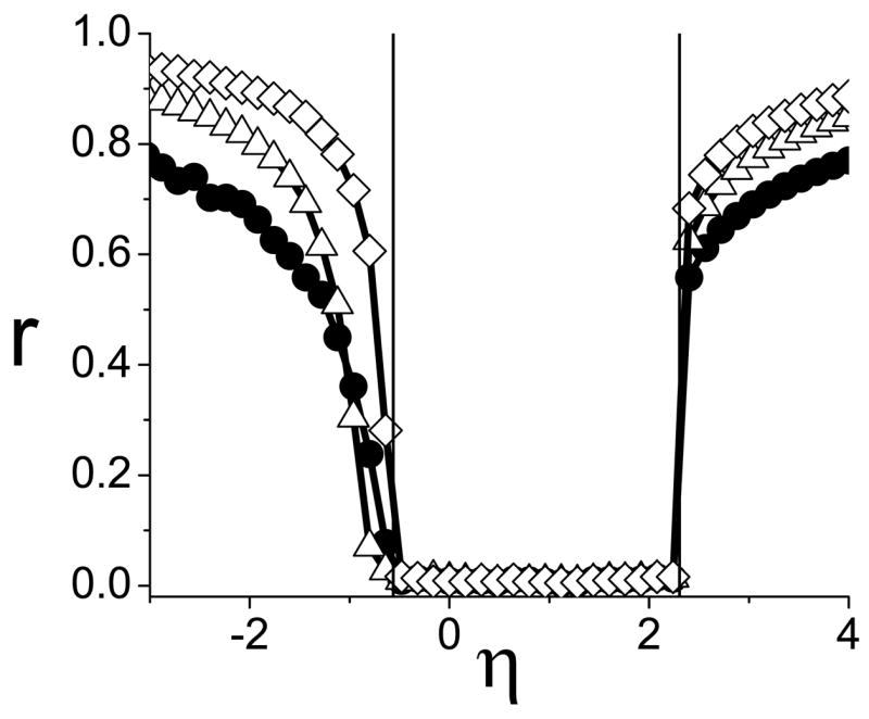
Three populations. Synchronization occurs at η* = −0.564 and 2.303, as predicted in Fig. (9).

References

- 1.Milo R, et al. Science. 2002;298:824–827. doi: 10.1126/science.298.5594.824. [DOI] [PubMed] [Google Scholar]
- 2.Newman MEJ, Girvan M. Phys Rev. 2004;E 69:026113. doi: 10.1103/PhysRevE.69.026113. [DOI] [PubMed] [Google Scholar]
- 3.Arenas A, Díaz-Guilera A, Pérez-Vicente CJ. Phys Rev Lett. 2006;96:114102. doi: 10.1103/PhysRevLett.96.114102. [DOI] [PubMed] [Google Scholar]; Arenas A, Díaz-Guilera A, Pérez-Vicente CJ. Physica D. 2006;224:27–34. [Google Scholar]
- 4.Kurant M, Thiran P. Phys Rev Lett. 2006;96:138701. doi: 10.1103/PhysRevLett.96.138701. [DOI] [PubMed] [Google Scholar]
- 5.Wang X, Huang L, Lai Y-C, Lai CH. Phys Rev. 2007;E 76:056113. doi: 10.1103/PhysRevE.76.056113. [DOI] [PubMed] [Google Scholar]
- 6.Zhou C, Zemanová L, Zamora G, Hilgetag CC, Kurths J. Phys Rev Lett. 2006;97:238103. doi: 10.1103/PhysRevLett.97.238103. [DOI] [PubMed] [Google Scholar]
- 7.Girvan M, Newman MEJ. Proc Natl Acad Sci. 2002;99:7821–7826. doi: 10.1073/pnas.122653799. [DOI] [PMC free article] [PubMed] [Google Scholar]
- 8.Milo R, et al. Science. 2004;303:1538–1542. doi: 10.1126/science.1089167. [DOI] [PubMed] [Google Scholar]
- 9.Kuramoto Y. International Symposium on Mathematical Problems in Theoretical Physics. In: Araki H, editor. Lecture Notes in Physics. Vol. 39. Springer; Berlin: 1975. [Google Scholar]; Chemical Oscillators, Waves and Turbulence. Springer; Berlin: 1984. [Google Scholar]
- 10.Winfree AT. The Geometry of Biological Time. Springer; New York: 1980. [Google Scholar]; Strogatz SH. Physica D. 2000;143:1. [Google Scholar]; Acebrón JA, et al. Rev Mod Phys. 77:137–185. [Google Scholar]; Wiesenfeld K, Swift JW. Phys Rev. 1995;E 51:1020–1025. doi: 10.1103/physreve.51.1020. [DOI] [PubMed] [Google Scholar]; Kiss IZ, Zhai Y, Hudson JL. Science. 2005;296:1676. doi: 10.1126/science.1070757. [DOI] [PubMed] [Google Scholar]
- 11.A similar system of two asymmetrically interacting populations with a particular form of coupling matrix K was considered in Montbrio E, Kurths J, Blasius B. Phys Rev. 2004;E 70:056125. doi: 10.1103/PhysRevE.70.056125. The formulation in the current paper is more general in two important aspects: K is arbitrary, and we allow for any number of interacting populations
- 12.Our system is similar to that studied in Restrepo JG, Ott E, Restrepo JG. Chaos. 2005;16:015107. However, our formulation permits different natural frequency distributions for each population
- 13.The bracketed expression is valid for Re(s) > 0 and may be analytically continued into the region where Re(s) ≤ 0. See Ott E, So P, Barreto E, Antonsen T. Physica D. 2002;173:226–258.Ott E. Chaos in Dynamical Systems. 2. Cambridge University Press; 2002. p. 240.
- 14.Many interesting states require ασσ′ ≠ = 0, such as the chimera state observed in Abrams DM, Strogatz SH. Int J Bif Chaos. 2006;16(1):21–37.
- 15.Simulations used fourth-order Runge-Kutta with a timestep of 0.01 seconds, N = 10, 000 or 50, 000, and parameters as noted. The system was initialized in the incoherent state and an initial transient was discarded. The order parameters were then averaged over the subsequent 10 seconds. Because the standard deviations over this interval were small, no error bars were plotted.
- 16.MATLAB®, The MathWorks, Inc., Natick, MA (http://www.mathworks.com/).