Efficiency of the human observer detecting random signals in random backgrounds

Abstract

The efficiencies of the human observer and the channelized-Hotelling observer relative to the ideal observer for signal-detection tasks are discussed. Both signal-known-exactly (SKE) tasks and signal-known-statistically (SKS) tasks are considered. Signal location is uncertain for the SKS tasks, and lumpy backgrounds are used for background uncertainty in both cases. Markov chain Monte Carlo methods are employed to determine ideal-observer performance on the detection tasks. Psychophysical studies are conducted to compute human-observer performance on the same tasks. Efficiency is computed as the squared ratio of the detectabilities of the observer of interest to the ideal observer. Human efficiencies are approximately 2.1% and 24%, respectively, for the SKE and SKS tasks. The results imply that human observers are not affected as much as the ideal observer by signal-location uncertainty even though the ideal observer outperforms the human observer for both tasks. Three different simplified pinhole imaging systems are simulated, and the humans and the model observers rank the systems in the same order for both the SKE and the SKS tasks.

1. INTRODUCTION

We take a task-based approach for image quality assessment. That is, we measure image quality on the basis of the performance of a particular observer on a particular task. The tasks of interest in medical imaging are either estimation tasks, where parameters of interest are estimated, or classification tasks, where a given image is classified into one of a set of defined categories. In this paper, we focus on a classification task, namely a two-alternative forced-choice (2AFC) signal-detection task. The 2AFC task gives an observer two stimuli, i.e., signal-absent and signal-present images, and forces the observer to identify which image has a signal.¹

In principle, human observers could be used to perform signal-detection tasks for system design or optimization. However, having human observers perform the tasks is too time-consuming for system design or optimization in practice. A good alternative is to use model observers such as Hotelling observers or ideal observers. The Hotelling observer maximizes the signal-to-noise ratio (SNR), which is a common measure of observer performance. The Hotelling observer constrained to a number of channels is called the channelized-Hotelling observer (CHO). The CHO using Laguerre–Gaussian (LG) channels has been shown to well approximate the Hotelling observer in terms of the SNR (see Ref. 2) when lumpy backgrounds and circularly symmetric signals are used for object variability. We will call this kind of CHO an efficient CHO (eCHO) since LG channels are used as efficient channels for the CHO to approximate the Hotelling observer. Other channels such as difference-of-Gaussian and Gabor channels are used for a CHO to model the human observer. The Bayesian ideal observer is optimal among all the observers, because it makes use of all the statistical information of the image data and sets an upper limit on the performance of any observer on the tasks. Thus the ideal observer gives a measure of the quality of image data.

The problem of estimating the ideal-observer test statistic has drawn considerable interest from the medical imaging community. However, in order to facilitate the computation of the ideal observer, backgrounds that had been used were too simplified to characterize realistic and complicated features in clinical images. Recently Kupinski et al.³ developed Markov chain Monte Carlo (MCMC) methods for estimating the likelihood ratio with random backgrounds and fixed Gaussian signals. Park et al.⁴ extended MCMC methods to the cases in which both backgrounds and signals are random. In these studies, the lumpy background, which was proposed by Rolland and Barrett,⁵ was used for background uncertainty. As Barrett et al.⁶ mentioned in their work, the lumpy background may accurately capture important features of real anatomical backgrounds at least for simple signal-detection tasks. Thus the lumpy background may still be a good choice for a random background, although more realistic and anatomical backgrounds are desired.

Human observers are inefficient, so they are unable to perform the detection tasks as well as the ideal observer. A source of human inefficiency is intrinsic uncertainty.⁷ Intrinsic uncertainty about signal characteristics such as intensity, location, and size may contribute to the degradation of the detection performance of the human observer compared with that of the ideal observer. Pelli⁸ studied uncertainty that explains the human-observer detection of contrast-defined signals. Moreover, it has been shown that the detection performance of the human observer is affected by inherent location uncertainty in the human visual system. Swensson and Judy⁹ used an extreme detector model for detecting spatially uncertain signals in noisy backgrounds in order to predict the performance degradation of the human observer for both signal-detection and localization tasks by increasing the number of possible signal locations. Manjeshwar and Wilson¹⁰ studied the effect of inherent location uncertainty on the detection of stationary targets in noisy images. Their studies showed that the detection performance of the human observer is degraded by inherent location uncertainty even in the signal-known-exactly (SKE) case in simplified backgrounds. That is, human observers act as if they are uncertain about the physical characteristics of the signal to be detected when the signal is exactly known. When a marker was added around the signal, the detection performance of the human observer improved by as much as 77%.

A detectability index and an efficiency expression were proposed by Tanner and Birdsall¹¹ as measures of observer performance. Human-observer detectability tells us how humans perform on the detection tasks. The efficiency is defined as the squared ratio of the detectability of the human observer to that of a standard observer. We use the Bayesian ideal observer as our standard observer since the ideal observer has the best achievable performance. The knowledge of the human-observer efficiency relative to the ideal observer is useful for system optimization because the efficiency reveals how much improvement is available to reach the best achievable performance. The human efficiency also tells us how much room we have available to develop and improve machine observers, which may be used for computer-aided diagnosis in the future. Therefore we are interested in measuring the efficiency of the human observer for performing signal-detection tasks.

Burgess et al.¹² measured the human efficiency relative to the ideal observer for detecting a SKE signal in spatially uncorrelated Gaussian noise. Burgess and Chandeharian¹³ conducted multiple-alternative forced-choice (MAFC) experiments using simple visual signals in uncorrelated image noise to calculate the human efficiency under signal-location uncertainty and found that the human efficiency is 50% for aperiodic signals. However, in these experiments, the backgrounds and signals were simplified in order to compute ideal-observer performance. More recently, Burgess et al.¹⁴ simulated image backgrounds with two-component noise; i.e., a background was generated by low-pass filtering of zero-mean Gaussian noise to simulate a statistically defined background, and then a component of white Gaussian noise was added to the resulting background to simulate image noise. Human-observer detectabilities of aperiodic signals were measured and were compared with those of various model observers including the Bayesian ideal observer. Both the noise and the background used in their experiments were independent stationary Gaussian random processes, and hence the sum of the noise and the background was also stationary Gaussian. This results in a linear Bayesian ideal observer for their experiments. Burgess et al.¹⁵ measured the human efficiency using the same types of lumpy backgrounds with power-law noise when the signal size was varied, and the signal contrast giving 90% correct responses for their 2AFC experiments was used. The average human efficiency relative to the ideal observer was about 40%. Burgess et al.¹⁵ also considered M statistically independent locations for MAFC experiments and found that the human efficiency for the MAFC experiments was about the same as for the 2AFC experiments. Bochud et al.¹⁶ did MAFC experiments similar to those of Burgess et al.¹⁵ to consider signal-location uncertainty and obtained similar results. Bochud et al. also discussed how to define M statistically independent locations more effectively by considering human perception of background characteristics.

By contrast, we generate the lumpy-background object with a Poisson random process and add Poisson measurement noise. Therefore the lumpy background for our studies may be non-Gaussian, so the ideal observer uses a nonlinear decision procedure.⁷ Signal-known-statistically (SKS) tasks, where both the background and signal-location are random, are compared with SKE tasks, where the signal is fixed and only the background is random. For our SKS tasks that consider signal-location uncertainty, signal locations are not statistically independent. We also simulate three simplified pinhole imaging systems in nuclear medicine and use the lumpy background as our object to be imaged by these systems to generate the image data for our studies. We shall see how observers rank these different imaging systems.

MCMC methods enable us to compare the performance of the human observer and the eCHO with the ideal observer and hence to quantify the efficiencies of the human observer and the eCHO on signal-detection tasks using lumpy backgrounds and random signals. For the comparison of observer performance, we conduct 2AFC psychophysical studies to obtain human-observer performance and employ MCMC methods to estimate the likelihood ratio for ideal-observer performance. The eCHOs are implemented using LG channels. We use a common figure of merit that is derived from the receiver-operating-characteristic (ROC) curve as our performance metric, the area under the ROC curve (AUC). The ROC curve can be generated by plotting the probability of detection (true-positive fraction) versus the false-alarm rate (false-positive fraction) varying the decision threshold. The AUC is an overall figure of merit without choosing a decision threshold. For 2AFC psychophysical studies, the AUC is the fraction of correct decisions, and the AUC for the eCHO can be estimated from the SNR. We measure the human and eCHO efficiencies relative to the ideal observer in the SKE cases as well as in the SKS cases.

2. MATHEMATICAL BACKGROUND

A. Imaging Process and Signal Detection

The imaging process can be written mathematically as

$$\mathbf{g}=\mathcal{H}\mathbf{f}+\mathbf{n},$$ (1)

where H is a continuous-to-discrete imaging operator that maps an object f to an M × 1 vector of image data g, f is a function of continuous variables, and n is an M × 1 vector of measurement noise with mean zero. That is, if our image is to be 128 × 128, the image and object vectors are 128² × 1. In nuclear medicine, the measurement noise is modeled to be conditionally Poisson on the mean image $\overline{\mathbf{g}}=\mathcal{H}\mathbf{f}$,

$$\text{pr}(\mathbf{g}\mid \overline{\mathbf{g}})=\prod _{m=1}^{M}exp(-{\overline{g}}_m)\frac{{\overline{g}}_m^{g_m}}{g_m!}.$$ (2)

A linear continuous-to-discrete imaging operator H can be written mathematically as

$$g_m={\int }_S\text{d}\mathbf{r}{h}_m(\mathbf{r})f(\mathbf{r})+n_m,$$ (3)

where r is a two-dimensional spatial coordinate, S is a field of view (FOV), h_m is the mth sensitivity function of H, and g_m and n_m are elements of g and n. Gaussian blur functions are used to simulate our simplified single-pinhole imaging systems^3,4:

$$h_m(\mathbf{r})=\frac{h}{2\pi w^2}exp\left[-\frac{{(\mathbf{r}-{\mathbf{p}}_m)}^{†}(\mathbf{r}-{\mathbf{p}}_m)}{2w^2}\right].$$ (4)

We use three different imaging systems A, B, and C with characteristics given in Table 1. The resolutions and relative sensitivities appearing in Table 1 correspond to different pinhole parameters and exposure times.

Table 1.

Characteristics of the Three Imaging Systems

Imaging System	Resolution w	Relative Sensitivity h
A	0.5	40
B	2.5	100
C	5	200

For 2AFC signal-detection tasks, we consider the tumor to be a signal f_s in a random background f_b, so the two hypotheses are given as

$$H_0:\mathbf{g}=\mathcal{H}{\mathbf{f}}_b+\mathbf{n},$$ (5)

$$H_1:\mathbf{g}=\mathcal{H}\text{(}{\mathbf{f}}_b+{\mathbf{f}}_s)+\mathbf{n}.$$ (6)

We define the background and signal image data to be $\mathbf{b}=\mathcal{H}{\mathbf{f}}_b$ and $\mathbf{s}=\mathcal{H}{\mathbf{f}}_s$ henceforth for notational convenience.

We generate an ensemble of signal-absent and signal-present images under both hypotheses and have the ideal observer, the human observer, and the eCHO perform the 2AFC signal-detection tasks in order to compare their performance.

B. Background and Signal Models

To describe background and signal uncertainty, we use statistical background and signal models. The lumpy background is written mathematically as⁵

$${\mathbf{f}}_b={\mathbf{f}}_b(\mathbf{r})=\sum _{n=1}^{N}L(\mathbf{r}-{\mathbf{c}}_n\mid a,s),$$ (7)

where r is a two-dimensional spatial coordinate, N is the random number of lumps in the object (Poisson with mean N̄), L(·) is the lump function, c_n is the center of the nth lump that is randomly chosen from a uniform distribution, and a and s are the fixed intensity and width of the lump function, respectively. The lump function L (·) is given by

$$L(\mathbf{r}-{\mathbf{c}}_n\mid a,s)=aexp\left[-\frac{{(\mathbf{r}-\mathbf{c})}^{†}(\mathbf{r}-\mathbf{c})}{2s^2}\right].$$ (8)

We use a = 1, s = 7, N̄ = 100, and M = 128² for M × 1 objects f, so the lumpy background images with these parameters are not well approximated by correlated Gaussian noise (see Fig. 1).

Fig. 1.

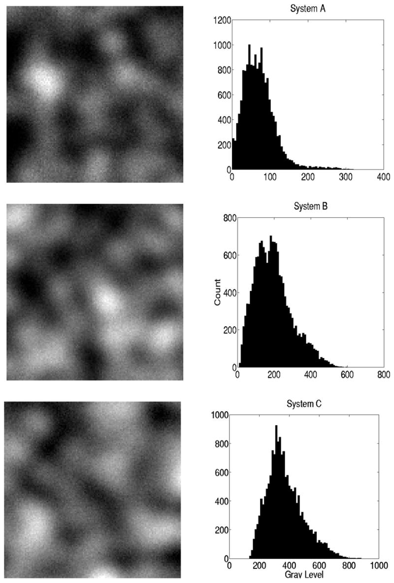
Gray-level histograms of three different lumpy backgrounds through the imaging systems A, B, and C.

The signal is written mathematically as⁴

$${\mathbf{f}}_s={\mathbf{f}}_s(\mathbf{r})=a_{s}exp\{-{[{\mathbf{R}}^{†}(\mathbf{r}-\mathbf{c})]}^{†}{\mathbf{D}}^{-1}[{\mathbf{R}}^{†}(\mathbf{r}-\mathbf{c})]\},$$ (9)

where a_s and c are the intensity and the center of the signal function, respectively; R is a rotation matrix; and D is a diagonal matrix whose diagonal entries are $2{\sigma }_1^2$ and $2{\sigma }_2^2$:

$$\mathbf{R}=\left[\begin{array}{cc}cos\theta & sin\theta \\ -sin\theta & cos\theta \end{array}\right],$$ (10)

$$\mathbf{D}=\left[\begin{array}{cc}2{\sigma }_1^2& 0\\ 0& 2{\sigma }_2^2\end{array}\right].$$ (11)

Signal-shape uncertainty can be considered by varying θ, σ₁, and σ₂. Park et al.⁴ use such signal models to include signal-shape uncertainty for estimating the ideal observer on various SKS detection tasks. In our experiments for SKS tasks, however, we consider only signal-location uncertainty and hence fix the shapes of the signals as circularly symmetric Gaussians; i.e., θ and σ₁(=σ₂) are constants, and we choose the locations of the signals from a uniform distribution in the FOV. For both the SKE and the SKS tasks, we used signal widths σ₁ = σ₂ = 3 and used a range of different signal intensities to fit their psychometric curves. The images of a fixed signal that are generated by the three different imaging systems are shown in Fig. 2.

Fig. 2.

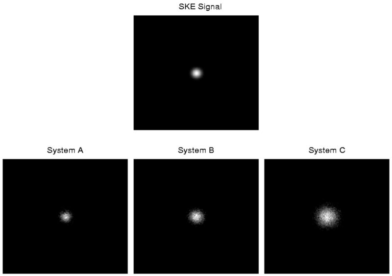
Images of a fixed signal through the three imaging systems A, B, and C.

3. METHODS

A. Ideal Observer

The ideal observer computes the likelihood ratio as its test statistic. The likelihood ratio is defined as

$$\mathrm{\Lambda }(\mathbf{g})=\frac{\text{pr}(\mathbf{g}\mid H_1)}{\text{pr}(\mathbf{g}\mid H_0)},$$ (12)

where pr(g|H_j) is the probability density of image data g under the hypothesis H_j.

1. Likelihood Ratio for Lumpy Backgrounds and Random Signals

As we consider the randomness of the background and the signal, the computation of the likelihood ratio in Eq. (12) becomes difficult. Because the background and the signal are random, we need to marginalize the conditional probabilities of the given data over the random background and random signal as follows:

$$\mathrm{\Lambda }(\mathbf{g})=\frac{\int \text{d}\mathbf{b}\int \text{d}\mathbf{s}\text{pr}(\mathbf{g}\mid \mathbf{b},\mathbf{s},H_1)\text{pr}(\mathbf{b})\text{pr}(\mathbf{s})}{\int \text{d}{\mathbf{b}}^{\prime }\text{pr}(\mathbf{g}\mid {\mathbf{b}}^{\prime },H_0)\text{pr}({\mathbf{b}}^{\prime })}.$$ (13)

Then the numerator and denominator in Eq. (13) are high-dimensional integrals. In order to estimate the likelihood ratio of the high-dimensional integrals more efficiently, MCMC methods have been developed for SKE-detection tasks by Kupinski et al.³ and extended for SKS-detection tasks by Park et al.⁴ We will summarize these methods below.

First, to reduce the high-dimension of the integrals in the likelihood ratio Eq. (13), we took advantage of our knowledge of the background and signal models. We defined parameter vectors θ to be {N, c₁, c₂,…,c_N} and α to be {c, θ, σ₁, σ₂}, respectively, for the background and signal models. The lumpy background b and the signal s are fully characterized by θ and α, respectively, and we assume that b and s are statistically independent of each other.

With this notation, we can write

$$\mathrm{\Lambda }(\mathbf{g})=\int \text{d}\mathit{\alpha }\int \text{d}\mathit{\theta }{\mathrm{\Lambda }}_{\text{BSKE}}(\mathbf{g}\mid \mathbf{b}(\mathit{\theta }),\mathbf{s}(\mathit{\alpha }))\text{pr}(\mathit{\theta }\mid \mathbf{g},H_0)\text{pr}(\mathit{\alpha }),$$ (14)

where Λ_BSKE, the likelihood ratio for background and signal known exactly (BSKE), is given by

$${\mathrm{\Lambda }}_{\text{BSKE}}(\mathbf{g}\mid \mathbf{b}(\mathit{\theta }),\mathbf{s}(\mathit{\alpha }))=\frac{\text{pr}(\mathbf{g}\mid \mathbf{b}(\mathit{\theta }),\mathbf{s}(\mathit{\alpha }),H_1)}{\text{pr}(\mathbf{g}\mid \mathbf{b}(\mathit{\theta }),H_0)},$$ (15)

and a posterior density in Eq. (14) is given by

$$\text{pr}(\mathit{\theta }\mid \mathbf{g},H_0)=\frac{\text{pr}(\mathbf{g}\mid \mathbf{b}(\mathit{\theta }),H_0)\text{pr}(\mathit{\theta })}{\int \text{d}{\mathit{\theta }}^{\prime }\text{pr}(\mathbf{g}\mid \mathbf{b}({\mathit{\theta }}^{\prime }),H_0)\text{pr}({\mathit{\theta }}^{\prime })}.$$ (16)

Likelihood ratio (14) is the posterior mean of Λ_BSKE, and we know how to compute Λ_BSKE from Poisson measurement noise, which is given as Eq. (2).

2. Computation of the Likelihood Ratio

Ideally, we would use the method of Monte Carlo integration to compute Eq. (14) as

$$\widehat{\mathrm{\Lambda }}(\mathbf{g})=\frac{1}{J}\sum _{j=1}^J{\mathrm{\Lambda }}_{\text{BSKE}}[\mathbf{g}\mid \mathbf{b}({\mathit{\theta }}^{(j)}),\mathbf{s}({\mathit{\alpha }}^{(j)})],$$ (17)

but pr(θ|g, H₀), from which we sample, is unknown. Therefore, MCMC methods are employed for estimating expectation (14) by means of Eq. (17).^3,4 In particular, we use the Metropolis–Hastings algorithms with symmetric proposal densities for pr(θ|g, H₀)pr(α).

A Markov chain is constructed with pr(θ|g, H₀)pr(α) as the stationary density for the chain. We can choose a proposal density q_b(θ| θ⁽ⁱ⁾)q_s(α| α⁽ⁱ⁾) for our Markov chain, where q_b(θ| θ⁽ⁱ⁾) and q_s(α| α⁽ⁱ⁾) are proposal densities, respectively, for pr(θ|g, H₀) and pr(α), because we assume that b and s are statistically independent of each other. To construct our Markov chain, given (θ⁽ⁱ⁾, α⁽ⁱ⁾), we draw a sample vector (θ̃, α̃) from the proposal densities and accept or reject it with acceptance probability

$$\begin{array}{l}\alpha (({\mathit{\theta }}^{(i)},{\mathit{\alpha }}^{(i)}),(\stackrel{\sim }{\mathit{\theta }},\stackrel{\sim }{\mathit{\alpha }}))\\ =min\left\{1,\frac{[\text{pr}(\stackrel{\sim }{\mathit{\theta }}\mid \mathbf{g},H_0)\text{pr}(\stackrel{\sim }{\mathit{\alpha }})][q_b({\mathit{\theta }}^{(i)}\mid \stackrel{\sim }{\mathit{\theta }})q_s({\mathit{\alpha }}^{(i)}\mid \stackrel{\sim }{\mathit{\alpha }})]}{[\text{pr}({\mathit{\theta }}^{(i)}\mid \mathbf{g},H_0)\text{pr}({\mathit{\alpha }}^{(i)})][q_b(\stackrel{\sim }{\mathit{\theta }}\mid {\mathit{\theta }}^{(i)})q_s(\stackrel{\sim }{\mathit{\alpha }}\mid {\mathit{\alpha }}^{(i)})]}\right\}.\end{array}$$ (18)

For q_s(α| α⁽ⁱ⁾), Park et al.⁴ used uniform distributions for choosing signal locations in the FOV; i.e., q_s(α| α⁽ⁱ⁾) = 1/M. Kupinski et al.³ designed a symmetric q_b(θ| θ⁽ⁱ⁾) for MCMC methods to estimate the likelihood ratio. Since the proposal densities are symmetric and the denominators of pr(θ̃|g, H₀) and pr(θ⁽ⁱ⁾|g, H₀) are the same as given in Eq. (16), we can rewrite the ratio in Eq. (18) into a computationally simpler one by canceling all q_b(θ| θ⁽ⁱ⁾), q_s(α| α⁽ⁱ⁾), pr(α), and the denominators; that is,

$$\frac{\text{pr}(\mathbf{g}\mid \mathbf{b}(\stackrel{\sim }{\mathit{\theta }}),H_0)\text{pr}(\stackrel{\sim }{\mathit{\theta }})}{\text{pr}(\mathbf{g}\mid \mathbf{b}({\mathit{\theta }}^{(i)}),H_0)\text{pr}({\mathit{\theta }}^{(i)})}.$$ (19)

The denominator and the numerator of ratio (19) are determined by the known distributions as follows:

$$\begin{array}{l}\text{pr}(\mathbf{g}\mid \mathbf{b}(\mathit{\theta }),H_0)\text{pr}(\mathit{\theta })=\text{pr}(\mathbf{g}\mid \mathbf{b}(\mathit{\theta }),H_0)\text{pr}(N)\text{pr}(\{{\mathbf{c}}_n\})\\ =\left\{\prod _{m=1}^{M}exp[-b_m(\theta )]\frac{b_m{(\theta )}^{g_m}}{g_m!}\right\}\\ \times \left[exp(-\overline{N})\frac{{\overline{N}}^N}{\overline{N}!}\right]\left[\frac{N!}{M^N}\right].\end{array}$$ (20)

Using MCMC methods, we estimate only one integral in Eq. (14) without having to calculate the denominator in Eq. (16), contrary to Eq. (13).

For each study of detection tasks with a signal intensity, we construct 400 Markov chains corresponding to 200 pairs of 128 × 128 signal-absent and signal-present images, estimate 400 corresponding likelihood ratios Λ̂(g), and then compute an estimate of the AUC, which would tell how well the ideal observer detects such a signal.

B. Human Observer

1. Psychophysical Studies

We have completed psychophysical studies for human-observer performance on the 2AFC signal-detection tasks, where signal and background uncertainties are present. A range of different signal intensities are used to fit psychometric functions for observer performance in the SKE and SKS cases.

One case at each level of signal intensity consisted of three studies for the three different imaging systems. On the study for each imaging system, observers were presented with 200 pairs of signal-absent and signal-present images after 100 trials of training. The lights were turned off in the room, where the experiments were performed, and a black background was used for the computer screen to reduce distractions to the observers. For each 2AFC detection task as shown in Fig. 3, three images were presented. A signal alone was presented in the middle image to show what the signal looks like. The other two images were random backgrounds with or without a signal, and the signal-present image was randomly on the left or right. The size of the images was 128 × 128 with a width of 35 mm on the display by Matlab software. A Cornea 17-in. CT 1700 LCD monitor was used for display. Luminance was measured by a Minolta CS-100 telephotometer. The mean luminances were 1.70 cd/m², 1.72 cd/m², and 3.66 cd/m², respectively, for imaging systems A, B, and C. The relation between gray level and luminance was a sigmoid curve, and our monitor was not linearized. Very low signal intensity may limit human contrast sensitivity because of the nearly flat shape of the sigmoid curve. However, none of the signal intensitiy values that were used for our experiments were low enough to fall into the nearly flat shape of the sigmoid curve. For the SKE cases, the signal is centered in the FOV, but for the SKS cases of signal-location uncertainty, the signal is not centered but randomly placed at one of 128² locations in the FOV. The observers were asked to choose which image had the signal. The observers were allowed unlimited time to reach a decision, and the viewing distance was not constrained.

Fig. 3.

2AFC signal-detection task.

Four observers participated in our studies, and none of them had any previous experience with 2AFC-detection experiments. To reduce an observer’s performance variability, a training session of 100 trials was conducted before the 200 actual trials began in each study. In these training trials, the observer was shown the result of each trial. The fraction of the observer’s correct responses was reported as well at the end of the trial session. We also disregarded the first few studies results for both the SKE and the SKS tasks, so that the observers were sufficiently familiar with the backgrounds and the signals over the whole studies with different levels of signal intensity.

2. Figure of Merit for Human-Observer Performance

For the performance of the human observer, we measure the fraction of correct decisions in the 2AFC experiment. It can be shown that the fraction of correct decisions is an estimate of the AUC,^7,17 and this derivation is reviewed below.

From the definition of the AUC and after manipulating the analytic form of the AUC, we get another form of the AUC given by¹⁷

$$\begin{array}{l}\text{AUC}={\int }_{\infty }{\text{d}}^{M}g{\int }_{\infty }{\text{d}}^M{g}^{\prime }\text{pr}(\mathbf{g}\mid H_0)\text{pr}({\mathbf{g}}^{\prime }\mid H_1)\\ \times \text{step}[\theta ({\mathbf{g}}^{\prime })-\theta (\mathbf{g})]\end{array}$$ (21)

where θ(g) is a test statistic and two independent data vectors g and g′ are drawn from H₀ and H₁, respectively.

For the human observer, we may consider θ(·) as a nonlinear discriminant function in the human visual system. Through the 2AFC psychophysical studies, the observers internally compute the two test statistics θ(g) and θ(g′), and they assign the data vector that gives the higher value to H₁. Their assignment is correct if θ(g′) > θ(g). Therefore the fraction of correct decisions is given by

$$Pr(\text{correct})=Pr[\theta ({\mathbf{g}}^{\prime })>\theta (\mathbf{g})]$$ (22)

$$\begin{array}{l}={\int }_{\infty }{\text{d}}^{M}g{\int }_{\infty }{\text{d}}^M{g}^{\prime }\text{pr}(\mathbf{g}\mid H_0)\text{pr}({\mathbf{g}}^{\prime }\mid H_1)\\ \times \text{step}[\theta ({\mathbf{g}}^{\prime })-\theta (\mathbf{g})],\end{array}$$ (23)

which is the AUC by Eq. (20).

C. Channelized-Hotelling Observer

The Hotelling observer uses the ensemble mean and covariance of the image data and maximizes the SNR, a measure of separability of the probability densities of the signal-present and signal-absent image data. The Hotelling template is linear and is given by⁷

$${\mathbf{w}}_{\mathbf{g}}={\mathbf{K}}_{\mathbf{g}}^{-1}\mathbf{s},$$ (24)

where w_g is an M × 1 vector, K_g is half the sum of the covariance matrices of the signal-absent and signal-present image data, and s is the difference between the mean signal-present and signal-absent image data; i.e.,

$$\mathbf{s}={\overline{\mathbf{g}}}_1-{\overline{\mathbf{g}}}_0,{\overline{\mathbf{g}}}_j=\langle \mathbf{g}\mid H_j\rangle ,j=0,1,$$ (25)

$$\begin{array}{l}{\mathbf{K}}_{\mathbf{g}}=\frac{1}{2}[{\mathbf{K}}_0+{\mathbf{K}}_1],\\ {\mathbf{K}}_j=\langle (\mathbf{g}-{\overline{\mathbf{g}}}_j){(\mathbf{g}-{\overline{\mathbf{g}}}_j)}^t\mid H_j\rangle .\end{array}$$ (26)

The test statistic for the Hotelling observer is computed by

$$t={\mathbf{w}}_{\mathbf{g}}^t\mathbf{g},$$ (27)

where g is under the signal-absent or the signal-present hypothesis. The AUC can be estimated directly from an ROC curve by use of this test statistic, and the SNR(= d_a) can be estimated by means of Eq. (37) below. Alternatively, given the Hotelling template, the SNR_Hot can be determined as⁷

$${\text{SNR}}_{\text{Hot}}^2={\mathbf{s}}^t{\mathbf{K}}_{\mathbf{g}}^{-1}\mathbf{s}.$$ (28)

If the test statistics under both hypotheses are Gaussian distributed, then SNR_Hot = d_a.

Since K_g is 16384 × 16384 for 128 × 128 (hence 16384 × 1) image data, the estimation of the Hotelling template is computationally burdensome, so we constrain the Hotelling observer to LG channels to construct the eCHO. We note that the eCHO is used not to model the human observer but to approximate the Hotelling observer by using LG channels as efficient channels. Gallas and Barrett² have shown that the eCHO approximates the Hotelling observer well in terms of the SNR when LG channels are used for lumpy backgrounds and circularly symmetric Gaussian signals; i.e., SNR_eCHO ≈ SNR_Hot, where SNR_eCHO represents the SNR for the eCHO.

Channel outputs v are defined as

$$\mathbf{v}=\mathbf{Tg}=\mathbf{T}(\mathcal{H}\mathbf{f}+\mathbf{n}),$$ (29)

where T is a channel matrix consisting of rows of M-dimensional channel vectors. The template w_v and the SNR_eCHO can be calculated with the covariance matrix of the channel outputs and the channel outputs of the signal as follows:

$${\mathbf{w}}_{\mathbf{v}}={\mathbf{K}}_{\mathbf{v}}^{-1}{\overline{\mathbf{s}}}_{\mathbf{v}},$$ (30)

$${\text{SNR}}_{\text{eCHO}}^2={\overline{\mathbf{s}}}_{\mathbf{v}}^t{\mathbf{K}}_{\mathbf{v}}^{-1}{\overline{\mathbf{s}}}_{\mathbf{v}},$$ (31)

$$\begin{array}{l}{\mathbf{K}}_{\mathbf{v}}=\mathbf{T}{\mathbf{K}}_{\mathbf{g}}{\mathbf{T}}^t,\\ {\overline{\mathbf{s}}}_{\mathbf{v}}={\langle {\mathbf{s}}_{\mathbf{v}}\rangle }_{\mathbf{s}},{\mathbf{s}}_{\mathbf{v}}=\mathbf{Ts}.\end{array}$$ (32)

For the SKE signal, s̄_v = s_v. The covariance matrix of the channel outputs can be computed as follows:

$${\mathbf{K}}_{\mathbf{v}}=\frac{1}{2}[{\mathbf{K}}_{\mathbf{v},0}+{\mathbf{K}}_{\mathbf{v},1}],$$ (33)

$${\mathbf{K}}_{\mathbf{v},0}=\mathbf{T}[\overline{\mathbf{b}}\mathbf{I}+{\mathbf{K}}_{\mathbf{b}}]{\mathbf{T}}^t,$$ (34)

$${\mathbf{K}}_{\mathbf{v},1}=\mathbf{T}[(\overline{\mathbf{b}}+\overline{\mathbf{s}})\mathbf{I}+{\mathbf{K}}_{\mathbf{b}}+{\mathbf{K}}_{\mathbf{s}}]{\mathbf{T}}^t$$ (35)

$$={\mathbf{K}}_{\mathbf{v},0}+\overline{\mathbf{s}}\mathbf{T}{\mathbf{T}}^t+\mathbf{T}{\mathbf{K}}_{\mathbf{s}}{\mathbf{T}}^t,$$ (36)

where K_v,0 and K_v,1 are the covariance matrices of the signal-absent and the signal-present channel outputs, respectively; K_b and K_s are the covariance matrices of the lumpy background and the signal, respectively; I is the identity matrix; and b̄ and s̄ are the mean background and mean signal, respectively.

For the SKE tasks, s̄ = s and K_s is a zero matrix. For the SKS tasks, s̄ = 〈s〉_s and the third term TK_sT^t in expression (36) is the covariance matrix of the channel outputs of the signal s_v, K_vs. For our 2AFC experiments, 20 LG channels were used; i.e., T is a 20 × 16384 matrix, and the channel outputs of 5000 training images were used to estimate K_v for each imaging system.

The eCHO performs poorly in detecting signals with location uncertainty. For the SKS tasks, the mean signal s̄_v in Eq. (30) is an average of an ensemble of signals over random signal locations, so the mean signal would be constant in theory. In other words, the difference between the mean signal-present and signal-absent image data is independent of spatial locations, so the eCHO template does not contain the information about where the signal is. This results in low performance of signal detection.

An alternative procedure¹⁸ may be employed to include signal-location uncertainty in the eCHO template. That is, an eCHO template for a SKE signal at each location is used to scan all 128² possible locations in the FOV to estimate the maximum linear discriminant t_max of all discriminants t over all the SKE signal locations. The t_max may be obtained at a location where the signal is most likely to be, but it may also be obtained at a location when the lump density is high. In the former case, this scanning eCHO would perform detection tasks better than the eCHO described earlier. In the latter case, the scanning eCHO template takes that false location as the signal location even though the signal is not there, which may result in low performance of signal detection. Note that we did not use this scanning scheme to incorporate signal-location uncertainty into the eCHO.

D. Detectability and Efficiency

For 2AFC signal-detection experiments, the detectability index d_a is related to the fraction of correct decisions (and hence AUC),

$$d_a\equiv 2{\text{erf}}^{-1}(2\text{AUC}-1),$$ (37)

where erf⁻¹ is the inverse of the error function. Note that this is merely a definition and does not imply that we are assuming Gaussian statistics.

To see how closely the human observer as well as the eCHO approximates the ideal observer in performance, we compare the AUC or detectability values for these observers. We also use observer efficiency to measure the perceptual efficiency of the human observer as well as the eCHO efficiency relative to the ideal observer. The efficiency e of an observer is defined as the squared ratio of the detectabilities of that observer to the ideal observer^11,12:

$$e={\left[\frac{d_a(·)}{d_a(\text{ideal})}\right]}^2.$$ (38)

E. Psychometric Function Fitting

1. Psychometric Functions

A psychometric function describes how an observer’s performance depends on some aspect of the physical stimulus. In our experiments, the physical stimulus is signal intensity. We are interested in comparing the performance of the human observer and the eCHO with that of the ideal observer when we vary signal intensity. Comparing psychometric functions for the human observer and the eCHO relative to the ideal observer with respect to signal intensity would be a reasonable way to compare their performance on the signal-detection tasks.

Plotting signal intensity versus observer performance gives a psychometric curve as long as enough data points for signal intensity and observer performance are provided. However, it is not feasible to measure observer performance at all levels of signal intensity for a continuous psychometric function, since it is too time-consuming to repeat psychophysical experiments for a large number of signal-intensity values. In practice, we can get only a small number of data points for both human-observer and ideal-observer performance. In order to fit psychometric functions with our experiment data using a small number of signal intensity values, we employ a maximum-likelihood (ML) method proposed by Wichmann and Hill.^19,20 We summarize their curve-fitting method for our experiments briefly in the following subsection.

2. Curve Fitting

We define K as the number of signal intensities used in our experiments, $\mathbf{x}={\{a_{\mathbf{s},i}\}}_{i=1}^K$ as a vector of signal intensities, and $\mathbf{n}={\{n_i\}}_{i=1}^K$ and $\mathbf{y}={\{y_i\}}_{i=1}^K$ as vectors of the number n_i of 2AFC trials and of observer performance y_i, respectively, at each level of signal intensity a_s,i. The y_i is the fraction of correct decisions for the 2AFC study using signal intensity a_s,i.

To model the process underlying the experimental data and fit psychometric curves, we used the method of ML estimation by Wichmann and Hill.^19,20 They assume the number of correct decisions y_in_i, given a signal intensity a_s,i, to be the sum of random samples from a Bernoulli process with a probability of success p_i. In order to specify the relationship between the underlying probability of a correct decision p and the signal intensity a_s, a general form is used given by

$$p=\psi (a_s;\alpha ,\beta ,\gamma ,\lambda )=\gamma +(1-\lambda -\gamma )F(a_s;\alpha ,\beta ),$$ (39)

where ψ (·) is a function from ℝ to ℝ and F is typically a sigmoid function such as the Weibull, logistic, cumulative Gaussian, or Gumbel distribution.¹⁹

The function F ranges in [0, 1]. The two parameters α and β of the function F determine the shape of the curve between the two bounds. We fix γ at 0.5 for our 2AFC detection experiments, which can be interpreted as the guess rate in the absence of a signal. The upper bound of the curve is 1 − λ, which is the performance level for a large signal intensity. The parameter λ reflects the rate of observers’ incorrect decisions regardless of signal intensity.

To estimate the three parameters, we define Ω as {α, β, λ} and the likelihood function $\mathcal{L}(\mathrm{\Omega };\mathbf{y})$ as the probability of having obtained y, given Ω; i.e.,

$$\begin{array}{l}\mathcal{L}(\mathrm{\Omega };\mathbf{y})=\prod _{i=1}^K\left(\begin{array}{c}{n}_i\\ y_i{n}_i\end{array}\right)\psi {(a_{s,i};\mathrm{\Omega })}^{y_i{n}_i}[1\\ -\psi (a_{s,i};\mathrm{\Omega }){]}^{(1-y_i)n_i}.\end{array}$$ (40)

The ML estimator Ω̂ of Ω is the set of three parameters that makes L largest for all Ω. The log-likelihood log $\mathcal{L}(\mathrm{\Omega };\mathbf{y})$ is maximized by the same estimator Ω̂ since the logarithm is monotonic. The log-likelihood log L is maximized by using the multidimensional Nelder–Mead simplex search algorithm.¹⁹ Bayesian priors W(Ω) are introduced in order to avoid inappropriate values for λ, such as a large λ or a negative λ. The case of a large λ can be interpreted to imply that the observer makes a large proportion of incorrect decisions no matter how strong the signal intensity, which means that the experiment was not performed properly.¹⁹ A negative λ means that an observer’s performance can exceed 100% correct, which does not make sense. Bayesian priors provide a mechanism for constraining parameters within realistic ranges on the basis of the experimenter’s prior beliefs about the likelihood of particular values.¹⁹ Finally, the fitting process maximizes $W(\mathrm{\Omega })\mathcal{L}(\mathrm{\Omega };\mathbf{y})$ or $logW+log\mathcal{L}$, rather than $\mathcal{L}(\mathrm{\Omega };\mathbf{y})$ or $log\mathcal{L}$. In other words, this process finds the maximum a posteriori estimator Ω̂.

For our experiments, we chose to use the Weibull function for F, since it has been widely used to fit psychometric curves throughout the literature.^21–23 The Weibull function is described by

$$F(x;\alpha ,\beta )=1-exp[-{(x/\alpha )}^{\beta }],0\le x<\infty ,$$ (41)

and a prior W(Ω) is used, given as¹⁹

$$W(\lambda )=\{\begin{array}{ll}1\hfill & \text{on}[0,0.05]\hfill \\ 0\hfill & \text{otherwise}\hfill \end{array}.$$ (42)

4. RESULTS

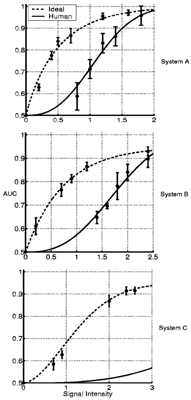
To estimate the likelihood ratio, the linear discriminant of the eCHO, and human-observer performance, 200 pairs of 128 × 128 signal-absent and signal-present images were used for the SKE and SKS detection tasks for each signal intensity and each imaging system. ROC analysis with LABROC4 (Ref. ²⁴) and PROPROC (Ref. ²⁵) software, and the 2AFC method¹⁷ were used to estimate the AUC values for three imaging systems for the ideal observer and the eCHO. For ideal-observer performance, we repeated the MCMC computation using different random-number seeds to calculate the sample variances of the AUC estimates.⁴ For human-observer performance, we calculated the fraction of correct decisions, which is an estimate of the AUC.¹⁷ After we estimated the AUC values for all the above observers, we fitted psychometric functions using PSIGNIFIT version 2.5.41, which implements Wichmann and Hill’s MLE method.¹⁹ From the fitted psychometric functions, observer efficiencies were calculated (see Figs. 4–6). However, the fitting scheme was not applied to the eCHO for the SKS tasks, owing to their poor performance; that is, their AUC values could not provide the proper shape of psychometric curves within signal-intensity values used in our experiments, as indicated in Fig. 6.

Fig. 4.

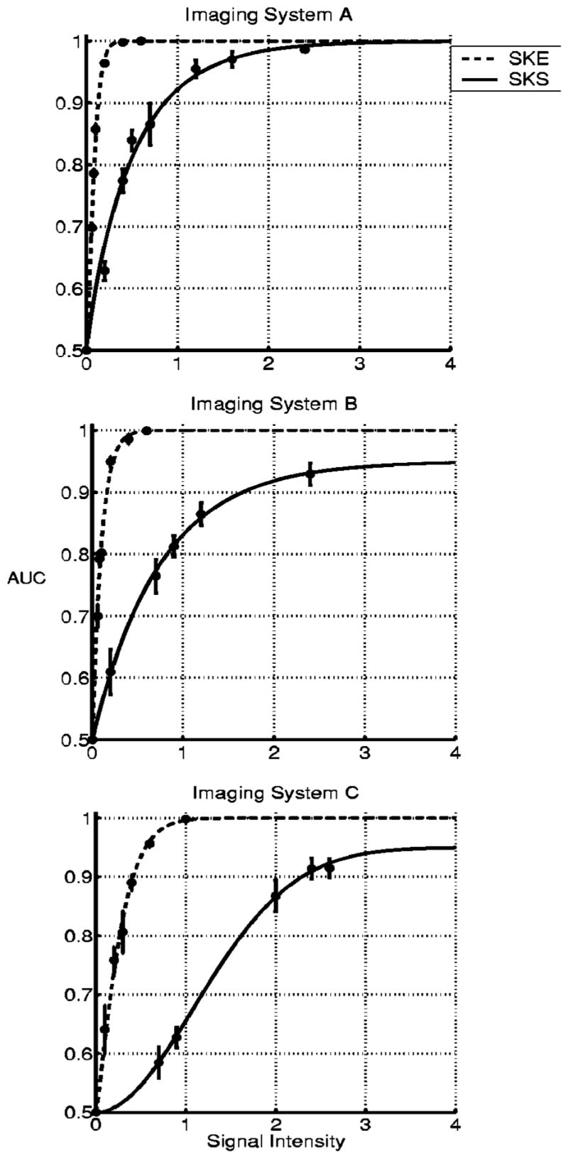
Psychometric curves for the ideal observer on the SKE and SKS tasks for each imaging system. The measured data points of observer performance and their error bars are provided.

Fig. 6.

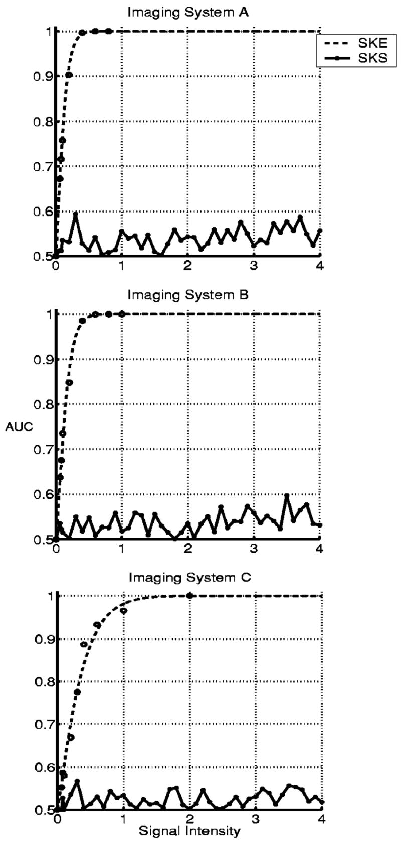
Psychometric curves for the eCHO on the SKE and SKS tasks for each imaging system. The measured data points of observer performance are provided.

The performance of the ideal observer, the human observer, and the eCHO reveals the rankings between imaging systems A, B, and C for performing the SKE signal-detection tasks in Fig. 7. The rankings remain the same, and the performance of each observer is highest on system A and lowest on system C. In Fig. 8 a comparison of the performance of the ideal observer and the human observer shows that the rankings among imaging systems A, B, and C for performing the SKS signal-detection tasks are the same as for the SKE tasks. However, the signal intensities that are needed to achieve certain observer performance are different depending on which observer and task are considered. The eCHO is not able to rank imaging systems for the SKS tasks, owing to its poor performance.

Fig. 7.

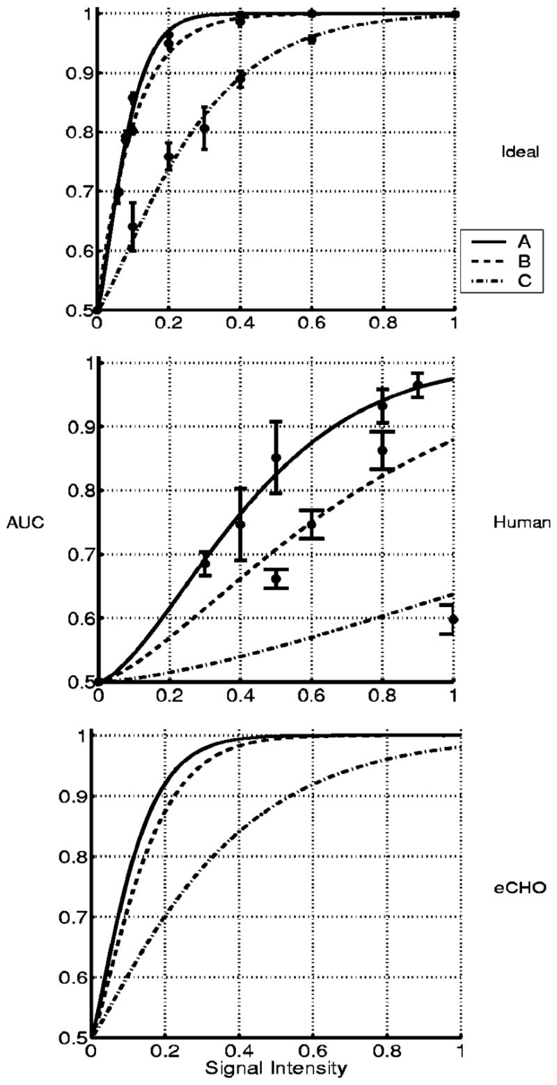
Psychometric curves for each observer on the SKE tasks for imaging systems A, B, and C.

Fig. 8.

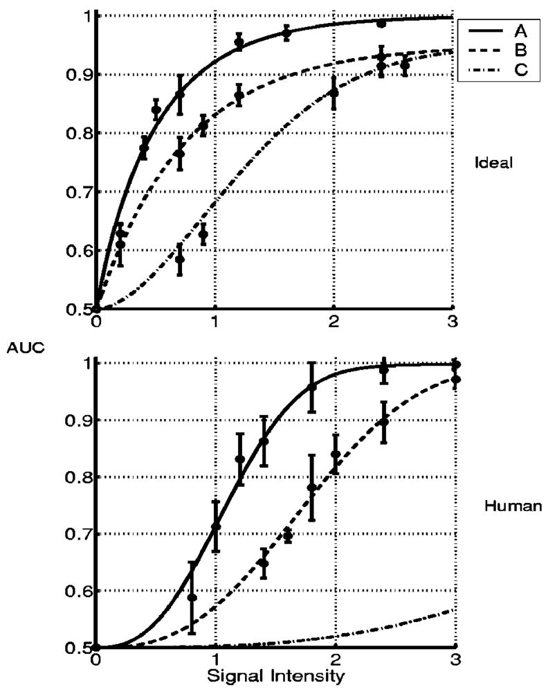
Psychometric curves for the ideal observer and the human observer on the SKS tasks for imaging systems A, B, and C.

Figures 4, 5, and 6 show that the performance of the ideal observer, the human observer, and the eCHO degrades when signal-location uncertainty is added to background uncertainty, while the ideal observer outperforms the human observer and the eCHO for each imaging system as shown in Figs. 9 and 10. Interestingly, human-observer performance is degraded less from ideal-observer performance for the SKS tasks than for the SKE tasks, as shown in Figs. 9 and 10. As a result, the human-observer efficiency is higher for the SKS tasks than for the SKE tasks.

Fig. 5.

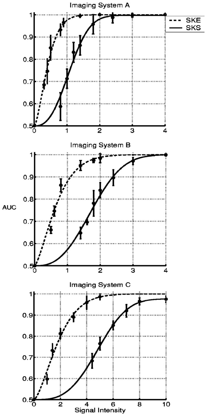
Psychometric curves for the human observer on the SKE and SKS tasks for each imaging system. The measured data points of observer performance and their error bars are provided.

Fig. 9.

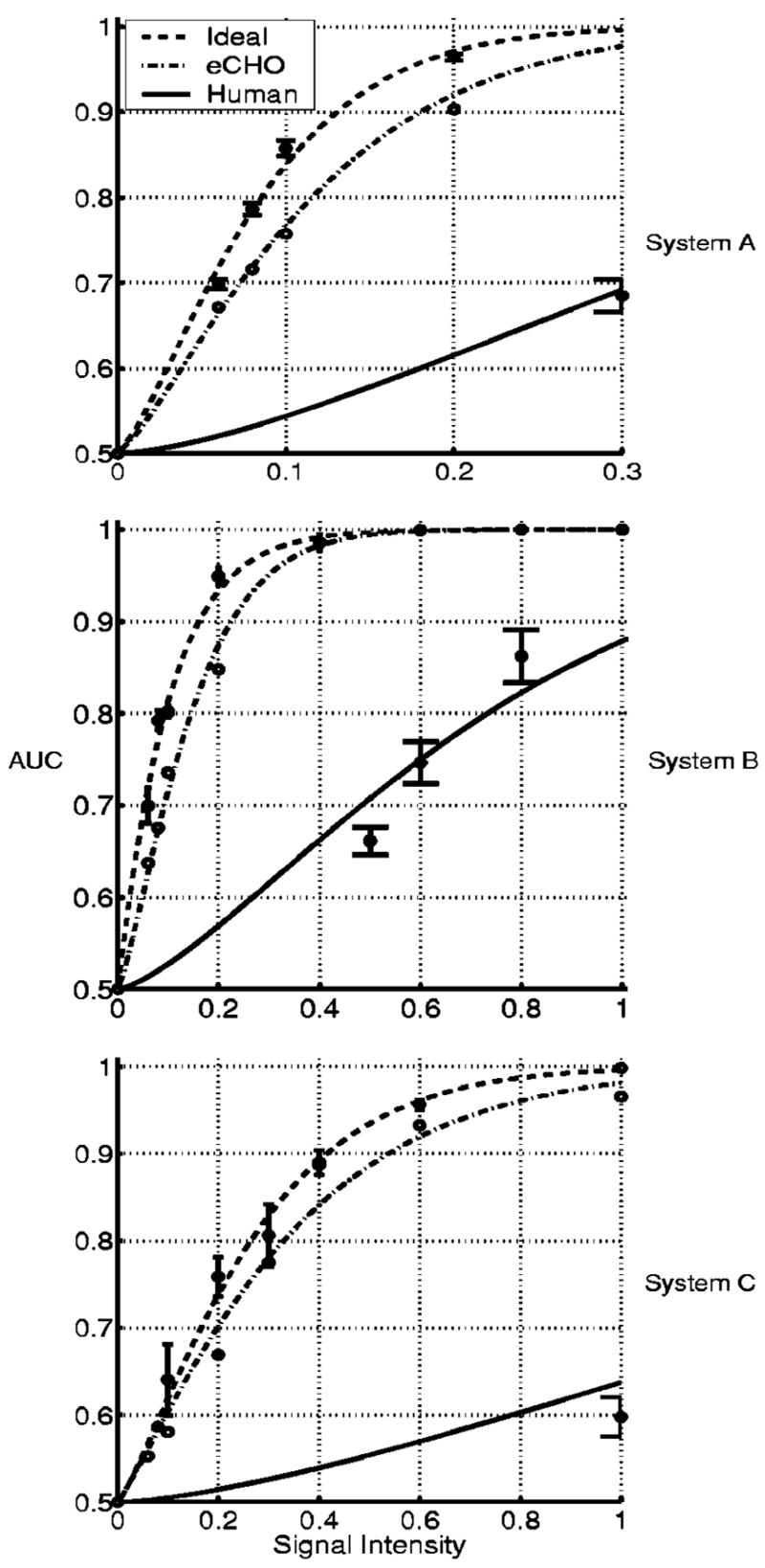
Psychometric curves for each imaging system on the SKE tasks.

Fig. 10.

Psychometric curves for each imaging system on the SKS tasks.

Figures 11 and 12 provide observer detectability for estimating the human and eCHO efficiencies shown in Fig. 13. The human efficiencies for the SKE tasks are less than 2.5% and 1.5% for the two best imaging systems, A and B, respectively, as indicated in Fig. 13(a). The human efficiencies for the SKS tasks are less than 41% and 13%, respectively, for imaging systems A and B, as shown in Fig. 13(b), but they are higher than 1.6%. The ranges of signal intensities for these figures are from 0.1 to 0.2 and from 0.8 to 1.4, respectively, in Figs. 13(a) and 13(b). In these ranges, the AUC for the ideal observer varies between 0.80 and 0.95, as indicated by Fig. 4. In particular, the efficiencies of the human observer are 2.1% and 24%, respectively, for the SKE and SKS tasks, when the AUC for the ideal observer is ~0.94 for both tasks with imaging system A. The above results imply that the human observer is not affected by signal-location uncertainty as much as the ideal observer is in performing the 2AFC signal-detection tasks.

Fig. 11.

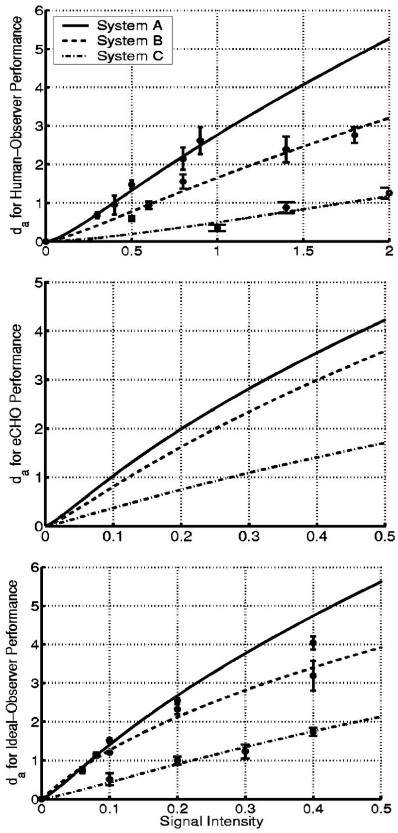
Observer detectability for the SKE tasks. The measured data points of observer performance and their error bars are provided.

Fig. 12.

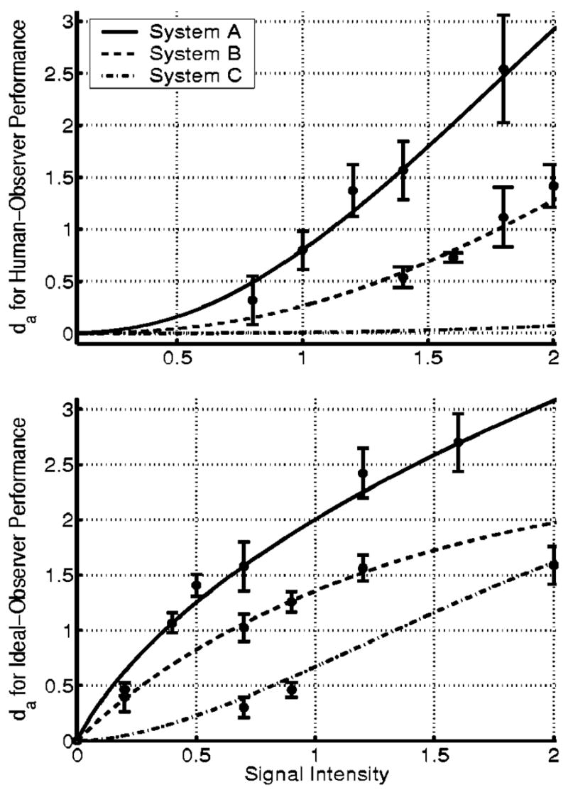
Observer detectability for the SKS tasks. The measured data points of observer performance and their error bars are provided.

Fig. 13.

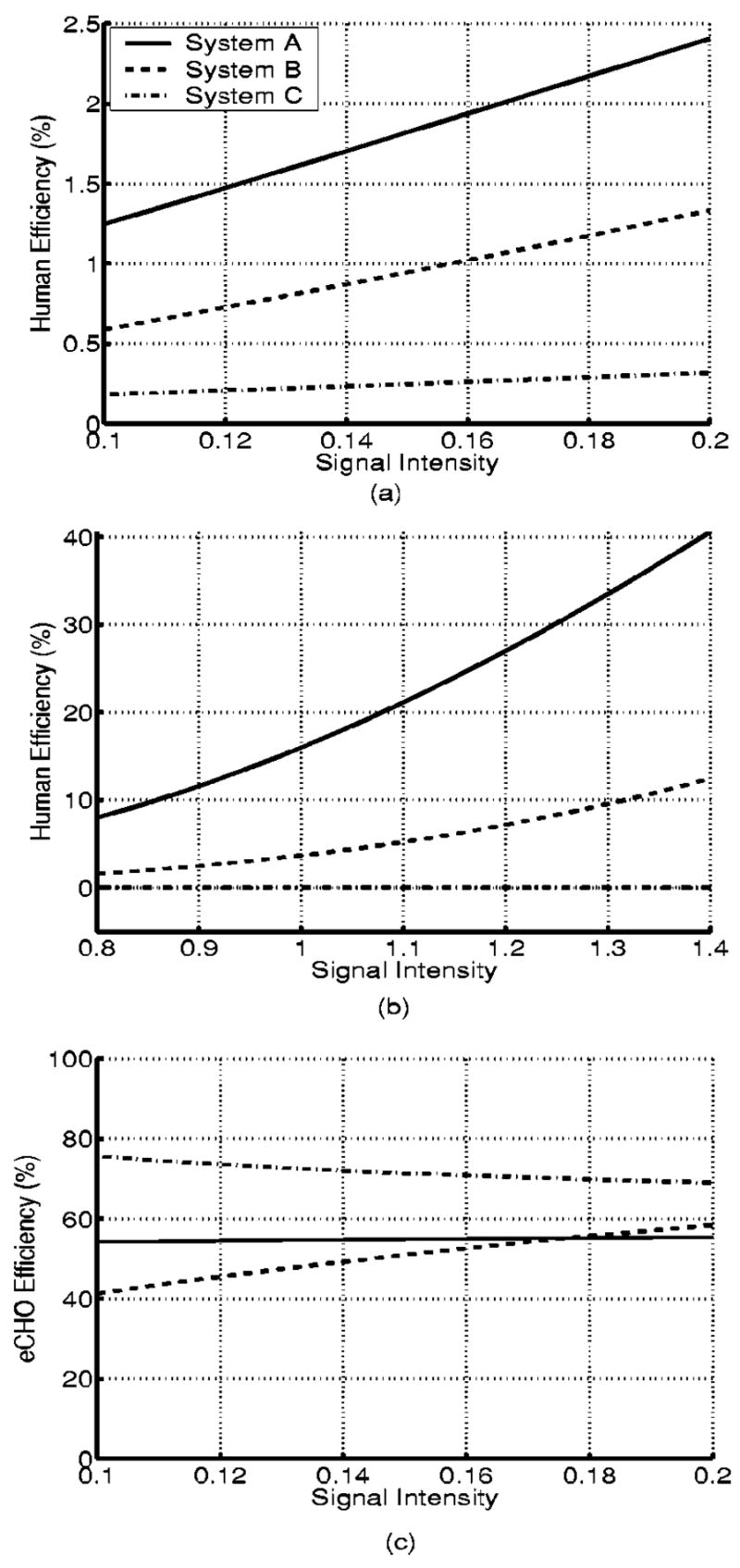
The human-observer efficiency for the SKE and SKS tasks and the eCHO efficiency for the SKE tasks for imaging systems A, B, and C. (a) SKE, (b) SKS, (c) SKE.

For imaging system C, the human efficiency for the SKE tasks is higher [<0.32% but >0.18% given in Fig. 13(a)] than for the SKS tasks [less than 0.047% in Fig. 13(b)]. However, the AUC for the ideal observer is small for system C, ranging from 0.60 to 0.75, for the SKE and SKS tasks as shown in Figs. 9 and 10, and the human efficiencies are too small to be significant. If we consider the range of the AUC for the ideal observer from 0.85 to 0.94 for the imaging system C for both the SKE and the SKS tasks, the estimated efficiency of the human observer varies between 0.52% and 0.84% for the SKE tasks and between 0.13% and 1.41% for the SKS tasks. Thus, contrary to the other systems, the human observer performs the SKE tasks better than the SKS tasks for system C, as the AUC of the ideal observer increases to 0.94 for both the SKE and SKS tasks. We believe that the human efficiency is compromised owing to the combined effect of high measurement noise in system C and signal-location uncertainty added to background uncertainty when signal intensity is not too strong.

In the range of signal intensities from 0.85 to 0.95 for systems A and B, the eCHO efficiencies for the SKE tasks are between 40% and 60% for both imaging systems, as indicated in Fig. 13(c). In particular, if the AUC for the ideal observer is approximately 0.94 for systems A and B, the eCHO efficiencies are 55% and 60%, respectively. The eCHO efficiency for imaging system C is between 70% and 80%, but the AUC for the ideal observer is from 0.6 to 0.73. When the AUC for the ideal observer varies from 0.85 to 0.95, the eCHO efficiency for system C ranges from 64% and 66%.

The eCHO outperforms the human observer on the SKE detection tasks for all imaging systems, as indicated by Fig. 9. However, for the SKS tasks with signal-location uncertainty, the human observer performs better than the eCHO, as shown in Figs. 5 and 6. The eCHO efficiency for the SKS tasks is less than 3% for imaging systems A and B, while the AUC for the ideal observer ranges from 0.80 to 0.95.

5. DISCUSSION AND CONCLUSIONS

We have estimated the human-observer efficiency relative to the ideal observer to show how well the human observer performs the 2AFC signal-detection tasks when the backgrounds and signal locations are random. The human efficiency for detecting the SKE and SKS signals in lumpy backgrounds has been shown to be small. Our results show that the ideal observer outperforms the human observer for both the SKE and the SKS tasks. However, the human observer is not affected by signal-location uncertainty as much as the ideal observer is, and this result is consistent with the past findings in the literature.^26–28 The human observer suffers from inherent location uncertainty, and the detection performance of the human observer is degraded by inherent location uncertainty even in SKE cases, so the addition of actual signal-location uncertainty would not degrade the performance of the human observer as much as that of the ideal observer.

The human efficiencies for the SKE tasks are approximately 2.1% and 1.6%, respectively, for the two best imaging systems, A and B, while the ideal observer performs well enough to get an AUC of ~0.94 for each system. The efficiencies on the SKS tasks are approximately 24% and 6%, respectively, for the two best imaging systems, A and B, while the AUCs for the ideal observer are ~0.94 and 0.85, respectively, for systems A and B. These results for the SKS tasks are consistent with those reported in the literature.¹⁵

The eCHO efficiencies relative to the ideal observer have been estimated as well for comparison with the human-observer efficiency. For the SKE tasks, they are between 50% and 60% when the AUC is 0.94 for systems A and B. The efficiencies are much higher than the human efficiency for the SKE tasks. However, the eCHO efficiencies for the SKS tasks are lower than 1% for all three imaging systems when the AUC is 0.95 for system A. They are much lower than the human efficiency for the SKS tasks.

The SKS tasks are more complicated and realistic than the SKE tasks, and the human observer performs the SKS tasks better than the eCHO. Furthermore, signal-location uncertainty does not affect human-observer performance as much as ideal-observer performance. However, the human efficiency is still low, so our results indicate that it is better to use the ideal observer for system optimization than the human observer or other model observers that predict the human-observer performance as long as we are aided by computational tools to estimate the ideal observer by using realistic backgrounds and signals. Therefore there is great potential for improvement of model observers that transcend human-observer performance.

References

- 1.Carpenter RHS, Robson JG, editors. Vision Research: A Practical Guide to Laboratory Methods. Oxford U. Press; New York: 1998. [Google Scholar]
- 2.Gallas BD, Barrett HH. Validating the use of channels to estimate the ideal linear observer. J Opt Soc Am. 2003;A 20:1725–1738. doi: 10.1364/josaa.20.001725. [DOI] [PubMed] [Google Scholar]
- 3.Kupinski MA, Hoppin JW, Clarkson E, Barrett HH. Ideal observer computation using Markov-chain Monte Carlo. J Opt Soc Am. 2003;A 20:430–438. doi: 10.1364/josaa.20.000430. [DOI] [PMC free article] [PubMed] [Google Scholar]
- 4.Park S, Kupinski MA, Clarkson E, Barrett HH. Ideal-observer performance under signal and background uncertainty. In: Taylor CJ, Noble JA, editors. Information Processing in Medical Imaging. Vol. 2732 of Lecture Notes in Computer Science. Springer-Verlag; New York: 2003. pp. 342–353. [DOI] [PubMed] [Google Scholar]
- 5.Rolland JP, Barrett HH. Effect of random background inhomogeneity on observer detection performance. J Opt Soc Am. 1992;A 9:649–658. doi: 10.1364/josaa.9.000649. [DOI] [PubMed] [Google Scholar]
- 6.Barrett HH, Abbey C, Gallas B, Eckstein M. Stabilized estimates of Hotelling-observer detection performance in patient-structured noise. Medical Imaging 1998: Image Perception. In: Kundel HL, editor. Proc SPIE 3340. Vol. 27. 1998. p. 43. [Google Scholar]
- 7.Barrett HH, Myers KJ. Foundations of Image Science. Wiley; New York: 2004. [Google Scholar]
- 8.Pelli DG. Uncertainty explains many aspects of visual contrast detection and discrimination. J Opt Soc Am. 1985;A 2:1508–1532. doi: 10.1364/josaa.2.001508. [DOI] [PubMed] [Google Scholar]
- 9.Swensson RG, Judy PF. Detection of noisy visual targets: Models for the effects of spatial uncertainty and signal-to-noise ratio. Percept Psychophys. 1981;29:521–534. doi: 10.3758/bf03207369. [DOI] [PubMed] [Google Scholar]
- 10.Manjeshwar RM, Wilson DL. Effect of inherent location uncertainty on detection of stationary targets in noisy image sequences. J Opt Soc Am. 2001;A 18:78–85. doi: 10.1364/josaa.18.000078. [DOI] [PubMed] [Google Scholar]
- 11.Tanner WP, Birdsall TG. Definitions of d′ and η as psychophysical measures. J Acoust Soc Am. 1958;30:922–928. [Google Scholar]
- 12.Burgess AE, Wagner RF, Jennings RJJ. Statistical efficiency: a measure of human visual signal detection performance. J Appl Photogr Eng. 1982;8:76–78. [Google Scholar]
- 13.Burgess AE, Chandharian H. Visual signal detection. II. Signal-location identification. J Opt Soc Am. 1984;A 1:906–910. doi: 10.1364/josaa.1.000906. [DOI] [PubMed] [Google Scholar]
- 14.Burgess AE, Xing Li, Abbey CK. Visual signal detectability with two noise components: anomalous masking effects. J Opt Soc Am. 1997;A 14:2420–2442. doi: 10.1364/josaa.14.002420. [DOI] [PubMed] [Google Scholar]
- 15.Burgess AE, Jacobson FL, Judy PF. Human observer detection experiments with mammograms and power-law noise. Med Phys. 2001;28:419–437. doi: 10.1118/1.1355308. [DOI] [PubMed] [Google Scholar]
- 16.Bochud FO, Abbey CK, Eckstein MP. Search for lesions in mammograms: statistical characterization of observer responses. Med Phys. 2004;31:24–36. doi: 10.1118/1.1630493. [DOI] [PubMed] [Google Scholar]
- 17.Barrett HH, Abbey CK, Clarkson E. Objective assessment of image quality III: ROC metrics, ideal observers, and likelihood-generating functions. J Opt Soc Am. 1998;A 15:1520–1535. doi: 10.1364/josaa.15.001520. [DOI] [PubMed] [Google Scholar]
- 18.Gifford HC, Pretorius PH, King MA. Comparison of human- and model-observer LROC studies. Medical Imaging 2003: Image Perception. In: Chakraborty DP, Krupinski EA, editors. Proc SPIE 5034. 2003. pp. 112–122. [Google Scholar]
- 19.Wichmann FA, Hill NJ. The psychometric function: I. Fitting, sampling, and goodness of fit. Percept Psychophys. 2001;63:1314–1329. doi: 10.3758/bf03194544. [DOI] [PubMed] [Google Scholar]
- 20.Wichmann FA, Hill NJ. The psychometric function: II. Bootstrap-based confidence intervals and sampling. Percept Psychophys. 2001;63:1314–1329. doi: 10.3758/bf03194545. [DOI] [PubMed] [Google Scholar]
- 21.Nachmias J. On the psychometric function for contrast detection. Vision Res. 1981;21:215–223. doi: 10.1016/0042-6989(81)90115-2. [DOI] [PubMed] [Google Scholar]
- 22.Quick RF. A vector magnitude model of contrast detection. Kybernetik. 1974;16:65–67. doi: 10.1007/BF00271628. [DOI] [PubMed] [Google Scholar]
- 23.Weibull W. Statistical distribution function of wide applicability. J Appl Mech. 1951;18:292–297. [Google Scholar]
- 24.Metz CE, Herman BA, Shen JH. Maximum likelihood estimation of receiver operating characteristic (ROC) curves from continuously-distributed data. Stat Med. 1998;17:1033–1053. doi: 10.1002/(sici)1097-0258(19980515)17:9<1033::aid-sim784>3.0.co;2-z. [DOI] [PubMed] [Google Scholar]
- 25.Metz CE, Pan X. Proper binormal ROC curves: theory and maximum-likelihood estimation. J Math Psychol. 1999;43:1–33. doi: 10.1006/jmps.1998.1218. [DOI] [PubMed] [Google Scholar]
- 26.Judy PF, Kijewski MF, Swensson RG. Observer detection performance loss: target size uncertainty. Medical Imaging 1997: Image Perception. In: Krupinski EA, Chakraborty DP, editors. Proc SPIE 3036. 1997. pp. 39–47. [Google Scholar]
- 27.Eckstein MP, Abbey CK. Model observers for signal-known-statistically tasks (SKS). Medical Imaging 2001: Image Perception. In: Krupinski EA, Chakraborty DP, editors. Proc SPIE 4324. 2001. pp. 91–102. [Google Scholar]
- 28.Zhang Y, Pham BT, Eckstein MP. Evaluation of JPEG 2000 encoder options: human and model observer detection of variable signals in X-ray coronary angiograms. IEEE Trans Med Imaging. 2004;23:613–632. doi: 10.1109/tmi.2004.826359. [DOI] [PubMed] [Google Scholar]