Avoiding bias from aggregate measures of exposure

Abstract

Background

Sometimes in descriptive epidemiology or in the evaluation of a health intervention policy change, proportions exposed to a risk factor or to an intervention are used as explanatory variables in log‐linear regressions for disease incidence or mortality.

Aim

To demonstrate how estimates from such models can be substantially inaccurate as estimates of the effect of the risk factor or intervention at individual level. To show how the individual level effect can be correctly estimated by excess relative risk models.

Methods

The problem and solution are demonstrated using data on prostate‐specific antigen testing and prostate cancer incidence.

In the past, temporal relationships between disease rates and potential risk factors estimated in ecological studies have given unexpected results.¹,²,³ This is likely to be due to unobserved confounding variables.¹ It may also be due to the bias engendered by using as an explanatory variable of the proportion exposed to a given factor in log‐linear or logistic regression analysis of aggregate rather than individual data. It is not well known that the use of the proportion exposed in such an analysis does not give the same estimates as would result from analysis of the effect of exposure at individual rather than aggregate level.

In this paper, we describe the principles of the potential bias, and show how it can be quantified. In addition, we develop methods for correct estimation of the individual relative risk (RR) from the aggregate data.

Methods

Usual individual‐level log‐linear model

Suppose that at individual level there is a relationship between risk of disease and exposure x given by

Ln(p) = α + βx

where p = risk (either probability or incidence rate) of disease and x = 0 if unexposed, x = 1 if exposed to a given risk factor. The quantity

R = exp(β)

is the RR of disease for an exposed subject compared to an unexposed. The quantity

p = exp(α)

is the risk of disease in subjects who are unexposed.

Use of aggregate data on exposure

Suppose that in a given period we do not know the risk factor status of individuals, but do know that a proportion φ of individuals were exposed to the risk factor. The unexposed subjects will have disease risk p, and the exposed will have risk Rp. The overall risk of disease in that period will be

P(D|φ) = φRp + (1−φ)p (1)

In a second period in which a proportion φ+h of individuals were exposed, the overall risk would be

P(D|φ+h) = (φ+h)Rp + (1−φ−h)p(2)

If we fit a log‐linear regression model with risk of disease as the dependent variable and proportion exposed as the explanatory variable, the regression model would be

log{P(D|φ)} = a+bφ(3)

Such a regression gives

exp(a+bφ) = P(D|φ)

and

exp(a+b(φ+h)) = P(D|φ+h)

Dividing equation (2) by the equation (1) gives

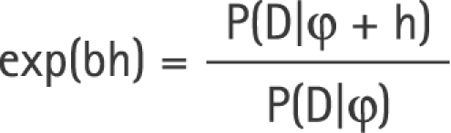Our estimate of the relative risk for exposure, R* = exp(b), will therefore have expectation

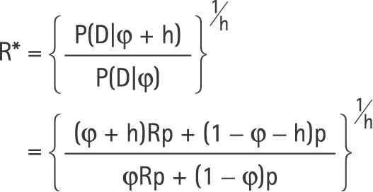Therefore,

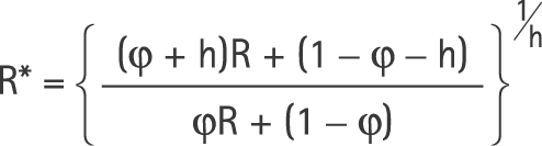Clearly, R* does not equal R, but additionally depends on the baseline risk and the proportions exposed. R* and R will be approximately equal if the arithmetic mean risk within any given period (as given in equation (1)) is approximately equal to the geometric mean as derived for equation (3).

In the case where there are only two periods, a closed‐form estimate of R, the true RR associated with individual exposure, can be derived by solving equation (4) for R. After a little algebra,

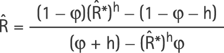where R̂* is the exponential of the estimated log‐linear regression coefficient for the proportion exposed.

Additive RR model

A closed‐form expression is not available where there are more than two periods. An alternative approach might be to attempt to estimate R using a software such as “R” where equation (1) can be fitted directly (code given in Appendix A), using product additive excess modelling, often referred to as excess RR, with fixed parameters, using the EPICURE software (code given in Appendix B).⁴,⁵,⁶

Consider a baseline period with exposure proportion φ as above, and average risk in that period as given in equation (1). Suppose there are k additional periods of observation with exposure proportions φ_i = φ+h_i(i = 1,…,k). For any given non‐baseline period i, the average risk is

P(D|φ+h_i) = (φ+h_i)Rp + (1−φ−h_i)p

 = φRp+(1−φ)p + h_i(R−1)p

 = P(D|φ) + (R−1)ph_i

Equation (1) can be written for any given φ_i as follows:

P(D|φ_i) = φ_ie^βe^a + (1−φ_i)e^a

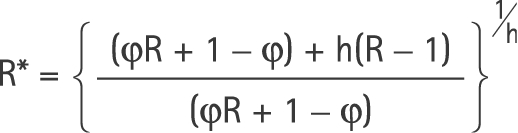
This can be re‐expressed in the form of an excess RR model, as defined by Breslow and Day,⁵ in chapter 4, as

P(D|φ_i) = e^a(1 + (e^β−1)φ_i)

 = e^a(1+(e^β−1)φ) + e^a(e^β−1)h_i

P(D|φ_i) + e^a(e^β−1)h_i

where P(D|φ_i) is the risk in the baseline category. Fitting such a model gives two estimates α̂, and β̂, from which we can, in turn, estimate p and R, by taking their exponentials. For further quantification of the relationship between the true R, the observed R* from traditional log linear regression on the proportion, and the absolute proportions exposed, see Discussion.

Demonstration 1: Simple example with fictitious data

Table 1 shows data from a simple example with two periods only.

Table 1 A simple fictitious dataset with two periods only.

Period	Cases	Period‐years	Proportion exposed
1	57	10455	0.20
2	100	9699	0.70

To generate the data, we calculate the expected numbers when the underlying disease rate for the unexposed is p = 0.0035 and when R = 3.77. For the two periods with φ = 0.2 and φ+h = 0.7, and period‐years of 10 455 and 9699, respectively, this gives the data in table 1. A conventional log‐linear regression analysis would give R̂* = 3.58.

Application of equation (5) gives the correct estimate of R,

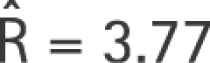Using the statistical package EPICURE⁶ with code given in Appendix B, the estimates of α and β in equation (6) were

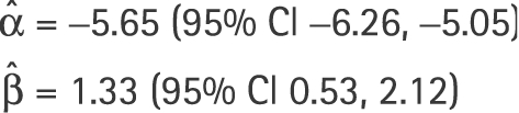This gives us estimates of p and R,

P^ = 0.0035 with 95% CI (0.0019 to 0.0065) and R^ = 3.77 (1.71 to 8.30)

The results estimated by the software “R” are identical. Thus, in this simple situation where the true result is already known, the excess RR model gives the correct estimates.

Demonstration 2: Example with more than two categories and no closed‐form solution

Table 2 shows incidence of prostate cancer in Cambridge, by 5 year age group, from 1996 to 2001 inclusive. It also shows the corresponding proportions of men exposed to prostate‐specific antigen testing. A conventional Poisson regression (using the numbers of cases and population at risk from which the incidence figures were calculated) of the proportion of men exposed to prostate‐specific antigen testing on prostate cancer risk gives a RR of 60.76 (95% CI 0.32 to 11 365).

Table 2 Prostate cancer cases, male population at risk and percentage exposed to prediagnostic prostate‐specific antigen testing in Cambridge, by age and calendar year.

Year	Cases						Population						Percentage exposed
	1996	1997	1998	1999	2000	2001	1996	1997	1998	1999	2000	2001	1996	1997	1998	1999	2000	2001
Age group
40–44	0	1	0	0	0	0	6175	6273	6432	6398	6549	6773	0.1	0.3	0.4	0.6	0.7	1.0
45–49	0	2	0	0	0	0	6677	6594	6284	6144	6024	6012	0.3	0.7	0.9	1.0	1.0	1.7
50–54	2	2	2	3	4	4	5298	5629	6247	6397	6261	6047	0.6	1.6	1.4	1.7	2.2	3.3
55–59	6	7	5	5	7	7	4385	4426	4606	4716	5166	5564	0.6	1.8	3.1	3.7	3.2	4.7
60–64	7	12	3	6	15	17	3763	3803	3968	4074	4079	4119	1.9	3.1	4.0	4.4	5.4	6.6
65–69	17	16	13	13	21	20	3443	3438	3422	3380	3419	3486	2.7	4.7	5.3	5.1	6.5	7.7
70–74	27	19	16	18	24	22	3027	2955	2979	3003	3076	3093	3.3	4.6	5.4	5.8	6.0	6.9
75–79	10	11	10	25	19	22	2209	2283	2462	2490	2380	2387	3.5	5.1	4.9	5.5	7.9	7.4
80–84	15	5	12	17	13	11	1518	1533	1400	1368	1553	1607	3.4	6.1	5.2	5.9	7.2	8.0
85–89	7	1	9	12	10	5	742	761	815	823	582	564	4.4	5.5	5.9	6.3	8.6	13.8
Total	91	76	70	99	113	108	37 237	37 695	38 615	38 793	39 089	39 652	20.8	33.5	36.5	40	48.7	61.1

The minimum exposure proportion was 0.001 and the maximum was 0.1383. This would give φ = 0.001 and h = 0.1373. Applying equation (5) gives R̂ = 6.57. However, this is only an approximation. The correct solution as given by the excess RR model in EPICURE, is R̂ = 6.51 (95% CI 1.58 to 26.66). Using the software “R”, the estimate is R̂ = 6.51 (95% CI 1.59 to 26.66).

Discussion

The above demonstrations show that regression of risk on the proportion exposed in a log‐linear model yields a RR estimate which can substantially differ from the RR associated with individual exposure. The inaccuracy can be an overestimate or an underestimate. It can also be substantial, as in the case of our example of prostate cancer. The latter is arguably an extreme example, as the exposure is very rare in this population and the association between exposure and risk is very strong. Table 3 shows the extent of the inaccuracy for a range of less‐extreme examples. Here, we set the values of R, φ and h and calculate the expected values of observed R. The essential relationship among the quantities φ, h, R* and R is defined by equations (4) and (5). Table 3 indicates that the bias from the naïve analysis is substantial and positive when the baseline prevalence is low and the difference in prevalences is high. This can be seen to be reasonable when we re‐express equation (4) as

Table 3 Observed RR estimate and its bias for traditional Poisson regression, for various values of R, φ and h*.

R	φ	h	Observed R	Bias (%)
1.5	0.05	0.1	1.62	+8
	0.2	0.2	1.55	+3
	0.2	0.6	1.49	−1
	0.5	0.2	1.47	−2
2.0	0.05	0.1	2.59	+30
	0.2	0.2	2.16	+8
	0.2	0.6	1.57	−2
	0.5	0.2	1.87	−7
2.5	0.05	0.1	3.69	+48
	0.2	0.2	2.82	+13
	0.2	0.6	2.40	−4
	0.5	0.2	2.21	−12

*R is true RR, φ is lowest observed proportion exposed, h is difference between the highest and lowest observed proportions.

What this paper adds

• This paper describes a common but often inappropriate interpretation of aggregate data in the analysis of descriptive studies that investigate associations between disease rates and population exposure. An easily applied and correct alternative is presented for epidemiologists.

The situation is more complicated when there are two aggregate proportions as explanatory variables, and one wishes to estimate a possible intervention between the two. Lasserre and colleagues⁷ developed complex models for when the proportion exposed to both factors is known, and for when it has to be estimated.

Clearly, the difference between the individual RR and that estimated by conventional log‐linear regression using the proportion exposed is potentially large enough to justify use of the excess RR model to derive an estimate of the former. It is frequently the case in descriptive epidemiology and other observational studies that only the proportion exposed at an aggregate level is available. The technique of excess RR estimation has been used to good effect in studies of radiation exposure.⁸,⁹ It is also likely to be useful in assessing the effects of health service interventions such as disease screening, or in the case of our example, the increased availability of diagnostic technology.

APPENDIX A. R code for maximum likelihood estimation of true R

Note that the package Stats4 must be loaded in order to carry out this estimation.

# store data in object demo1

#

demo1<‐data.frame(d = c(57, 100), py = c(10455, 9699),pe = c(0.2,0.7))

#

# construct ‐log likelihood function and starting values for iterative estimation‐ see equation (6)

# and preceding material

# mll<‐function(alfa = ‐5, beta = 0)

‐sum(dpois(demo1$d,

lambda = exp(alfa+log(demo1$py))*(1+demo1$pe*exp(beta)‐demo1$pe), log = TRUE))

#

# estimation by maximum likelihood

#

res<‐mle(mll)

#

# show results

#

summary(res)

APPENDIX B. EPICURE code for excess RR estimation

! input data

!

names d py pe@

records 2@

input <@

57 10455 0.2

100 9699 0.7

!

! define period‐years and cases

!

pyr py@

cases d@

!

! define a product additive excess model in the

! form of a constant intercept

! times (1+ a function composed of a linear and

! a log‐linear subterm) as in equation (6)

! the parameters for the exposed proportion (pe) are fixed

!

loglinear 0@

linear 1 pe = 1@

loglinear 1 %con@

linear 2 pe = ‐1@

fit

References

- 1.Tulinius H, Day N E, Johannesson G.et al Reproductive factors and risk for breast cancer in Iceland. Int J Cancer 197821724–730. [DOI] [PubMed] [Google Scholar]
- 2.Ewertz M, Duffy S W. Incidence of female breast cancer in relation to prevalence of risk factors in Denmark. Int J Cancer 199456783–787. [DOI] [PubMed] [Google Scholar]
- 3.Kojo K, Jansen C T, Nybom P.et al Population exposure to ultraviolet radiation in Finland 1920–1995: exposure trends and a time‐series analysis of exposure and cutaneous melanoma incidence. Environ Res 2006101123–131. [DOI] [PubMed] [Google Scholar]
- 4.Venables W N, Ripley B D.Modern applied statistics with S. New York: Springer, 2002
- 5.Breslow N E, Day N E. The design and analysis of cohort studies. Statistical methods in cancer research. Vol II. Lyon: IARC Scientific Publications, 1987 [PubMed]
- 6.Preston D L, Lubin J H, Pierce D A.et alEPICURE user's guide. Seattle: Hirosoft International Corporation, 1988–93
- 7.Lasserre V, Guihenneuc‐Jouyaux C, Richardson S. Biases in ecological studies: utility of including within‐area distribution of confounders. Stat Med 20001945–59. [DOI] [PubMed] [Google Scholar]
- 8.Howe G R, McLaughlin J. Breast cancer mortality between 1950 and 1987 after exposure to fractionated moderate‐dose‐rate ionizing radiation in the Canadian fluoroscopy cohort study and a comparison with breast cancer mortality in the atomic bomb survivors study. Radiat Res 1996145694–707. [PubMed] [Google Scholar]
- 9.National Research Council Committee on Health Risks of Exposure to Radon. BEIR VI. Health effects of exposure to radon Washington, DC: National Academy Press, 199969–85.