On Using Truncated Sequential Probability Ratio Test Boundaries for Monte Carlo Implementation of Hypothesis Tests

Abstract

When designing programs or software for the implementation of Monte Carlo (MC) hypothesis tests, we can save computation time by using sequential stopping boundaries. Such boundaries imply stopping resampling after relatively few replications if the early replications indicate a very large or very small p-value. We study a truncated sequential probability ratio test (SPRT) boundary and provide a tractable algorithm to implement it. We review two properties desired of any MC p-value, the validity of the p-value and a small resampling risk, where resampling risk is the probability that the accept/reject decision will be different than the decision from complete enumeration. We show how the algorithm can be used to calculate a valid p-value and confidence intervals for any truncated SPRT boundary. We show that a class of SPRT boundaries is minimax with respect to resampling risk and recommend a truncated version of boundaries in that class by comparing their resampling risk (RR) to the RR of fixed boundaries with the same maximum resample size. We study the lack of validity of some simple estimators of p-values and offer a new simple valid p-value for the recommended truncated SPRT boundary. We explore the use of these methods in a practical example and provide the MChtest R package to perform the methods.

1 Introduction

This paper is concerned with designing Monte Carlo implementation of hypothesis tests. Common examples of such tests are bootstrap or permutation tests. We focus on general hypothesis tests without imposing any special structure on the hypothesis except the very minimal requirement that it is straightforward to create the Monte Carlo replicates under the null hypothesis. Thus, for example, we do not require either special data structures needed to perform network algorithms (see, e.g., Agresti, 1992) nor knowledge of a reasonable importance sampling function needed to perform importance sampling (see, e.g., Mehta, Patel, and Senchaudhuri, 1988, or Efron and Tibshirani, 1993).

Let any Monte Carlo implementation of a hypothesis test be called an MC test. When using an MC test with a fixed number of Monte Carlo replications, often one will know with high probability, before completing all replications, whether the test will be significant or not. Thus, it makes sense to explore sequential procedures in this situation. In this paper we propose using a truncated sequential probability ratio test (SPRT) for MC tests. This is simply the usual SPRT except we define a bound on the number of replications instead of allowing an infinite number.

For estimating a p-value from an MC test, we show that the simple maximum likelihood estimate or the more complicated unbiased estimate (Girshick, Mosteller, and Savage, 1946), are not necessarily the best estimators since they do not produce valid p-values. We show how for any finite MC test (i.e., one with a predetermined maximum number of replications) we can calculate a valid p-value. The method depends on the calculation of the number of ways to reach each point on the stopping boundary of the MC test, and we present an algorithm to aid in the speed of that calculation for the truncated SPRT boundary.

Fay and Follmann (2002) explored MC tests and defined the resampling risk as the probability that the accept/reject decision will be different from a theoretical MC test with an infinite number of replications. Here we show that based on Wald’s (1947) power approximation there exists a class of SPRT tests which are minimax with respect to the resampling risk. This improves upon Lock (1991) who explored the SPRT for use in MC tests but made recommendations for SPRT’s which were not minimax. Then we propose truncating the chosen SPRT to prevent the possibility of a very large replication number for the MC test. For a similar truncated SPRT, Armitage (1958) has outlined a method for calculating exact confidence intervals for the p-value, and here we show how our algorithm is used in that situation also.

The paper is organized as follows. In Section 2 we present the problem and introduce notation. We review the SPRT in Section 3 and some results for finite stopping boundaries in Section 4. In Section 5 we discuss validity of the p-values from the MC test. In Section 6 we discuss the resampling risk and show that a certain class of SPRT boundaries are minimax with respect to the resampling risk. We compare truncated SPRT (tSPRT) boundaries with the associated fixed boundary having the same maximum resample size and recommend a specific tSPRT boundary when the significance level is 0.05. In Section 7 we show the lack of validity of some simple p-value estimators when used with truncated SPRT boundaries and propose a simple valid p-value for use with the recommended tSPRT boundary. In Section 8 we compare the use of a truncated SPRT boundary and a fixed resample size boundary in some examples. We explore the timings and p-values from both methods. In Section 9 we discuss some additional issues related to MC tests.

2 Estimating P-values by Monte Carlo Simulation

Consider a test statistic, T, for which larger values indicate more unlikely values under the null hypothesis. Let T₀ = T (d₀) denote the value of the test statistic applied to the original data, d₀. The Monte Carlo test may be represented as taking repeated independent replications from the data (e.g., bootstrap resamples, or permutation resamples), say d₁, d₂, …, and obtaining T₁ = T (d₁), T₂ = T (d₂),…. Under this Monte Carlo scheme the T_i are independent and identically distributed (iid) random variables from some distribution such that Pr[T_i ≥ T₀|d₀] = p(d₀) for all i, where the p(d₀) is the p-value that would be obtained if an infinite Monte Carlo sample or a complete enumeration was taken. So our problem may be reduced to the familiar problem of estimating a Bernoulli parameter p ≡ p(d₀), from many iid binary random variables X_i = I(T_i ≥ T₀), where I(A) is the indicator of an event A. Let $S_n={\sum }_{i=1}^n{X}_i$. Then X_i has a Bernoulli distribution with success probability of p for each i, and S_n has a binomial distribution with parameters n and p for a fixed n. However, we are interested in more general stopping rules to achieve a more efficient decision, and allow the number of Monte Carlo samples, N, to be a random variable.

We want to satisfy two properties of an estimator of p. First, we want the estimator to produce a valid p-value for the Monte Carlo test. Second, we want to minimize in some way both the probability that we conclude that p > α when p ≤ α and the probability that we conclude that p ≤ α when p > α, where α is the significance level of the Monte Carlo test. Before discussing these two properties in Sections 5 and 6 we review SPRT stopping boundaries in Section 3 and finite stopping boundaries (i.e., boundaries with a known maximum possible resample size) in Section 4.

3 Review of the Sequential Probability Ratio Test

Consider the sequential probability ratio test. We formulate the MC test problem in terms of a hypothesis test: H_0: p > α versus H_a: p ≤ α. Note that the equality is in the alternative, since traditionally we reject in an MC test when p = α. This is a composite hypothesis, and the classical solution (Wald, 1947) is to transform the problem to testing between two simple hypotheses based on two parameters p_a < α < p₀, and then perform the associated SPRT. Let λ_N be the likelihood ratio after N observations. The SPRT requires choosing constants A and B such that we stop the first time either λ_N ≤ B (in which case we accept H_0: p = p₀) or λ_N ≥ A (in which case we reject H₀). Equivalently, the SPRT says to stop the first time either

$$S_N\ge C_1+N{C}_0,$$

(then accept H_0: p = p₀) or

$$S_N\le C_2+N{C}_0,$$

(then reject H₀) where $C_0=log\left(\frac{1-p_0}{1-p_a}\right)/log(r)$, C₁ = log (B)/log (r) , C₂ = log (A)/log (r), and r = {p_a(1 − p₀)}/{p₀(1 − p_a)}. Note that the SPRT is overparametrized in the sense that there are 4 parameters p₀, p_a, A and B, but the SPRT can be defined by 3 parameters C₀, C₁, and C₂. In other words, we can define equivalent SPRT for different pairs of p₀ and p_a by changing A and B accordingly as long as C₀ remains fixed. For example, the following pairs of (p₀, p_a) all give C₀ = 0.05: (.061, .040), (.077, .030), and (.099, .020). We show contours of potentially equivalent SPRT in Figure 1.

Figure 1.

Contours of values of p₀ and p_a with equivalent values of C₀.

The SPRT minimizes the expected sample size both under the null, p = p₀, and the alternative, p = p_a, among tests with the same size and power for testing between those two simple point hypotheses (see e.g., Siegmund, 1985). Wald (1947) has shown that in order to approximately bound the type I error (conclude p = p_a when in fact p = p₀) at some nominal level, say α₀, and the type II error (conclude p = p₀ when in fact p = p_a) at some nominal level, say β₀, then one should use A = (1 − β₀)/α₀ and B = β₀/(1 − α₀). These approximate boundaries are called the Wald boundaries (see e.g., Eisenberg and Ghosh, 1991). Note that α₀ (the nominal level for the type I error of null hypothesis H_0: p = p₀ from the SPRT) is different from α (the significance level of the MC test).

Wald (1947) gave approximation methods for estimating the power function at any p and the expected [re]sample size. We reproduce those approximations and use them in Section 6.

4 Finite Stopping Boundaries

Now consider finite stopping rules which may be represented by the stopping boundary denoted by a b × 2 matrix,

$$B=\left[\begin{array}{ll}{\text{S}}_1\hfill & {\text{N}}_1\hfill \\ {\text{S}}_2\hfill & {\text{N}}_2\hfill \\ ⋮\hfill & ⋮\hfill \\ {\text{S}}_b\hfill & {\text{N}}_b\hfill \end{array}\right].$$

We continue with the Monte Carlo resampling (creating S₁, S₂,…) until N = N_j and S_N = S_j for some j, at which time the Monte Carlo simulation is stopped. We consider only boundaries for which when resampling is done as described above, the probability of stopping on the boundary is one for any p. Following Girshick, Mosteller, and Savage (1946) we call such boundaries closed. Further, we write the boundaries minimally, such that for any 0 < p < 1 the probability of stopping at any boundary point is greater than 0.

Figure 2 shows two finite boundaries. The boundary depicted by the dotted line represents the boundary of Besag and Clifford (1991) where we stop if S_N = s_max or if N = n_max. The boundary depicted by the solid line is the focus of this paper, the truncated sequential probability ratio test boundary. In that case most values of N_j on B are not unique, appearing on both the “upper” and the “lower” boundaries. The decision at any stopping point will be based on the estimated p-value at that point, and we discuss p-value estimation later.

Figure 2.

Plot of two stopping boundaries: truncated sequential probability ratio test (tSPRT) boundary with m = 9999, p_a = .04 and p₀ = .0614 (so that C₀ = .05) using the Wald boundaries with α₀ = β₀ = .0001 (solid black), and Besag and Clifford (1991) boundary with s_max = 499 and n_max = 9999 (dotted gray).

Let (S_N, N) be a random variable representing the final value of the Monte Carlo resampling associated with the finite boundary, B, and a p-value, p. We can write the probability distribution of (S_N, N) as

$$f_j(p,\mathit{B})\equiv Pr[S_N={\text{S}}_j,N={\text{N}}_j;p,\mathit{B}]=K_j(\mathit{B})p^{{\text{S}}_j}{(1-p)}^{{\text{N}}_j-{\text{S}}_j}$$ (1)

where K_j(B) is the number of possible ways to reach (S_j, N_j) under B.

In this situation, the simplest estimator of p is the maximum likelihood estimator (MLE), p̂_MLE(S_N, N) = S_N/N; however, the MLE is biased. Girshick, Mosteller, and Savage (1946, Theorem 7) showed that the unique unbiased estimator of p for all the boundaries considered in this paper (i.e., boundaries that are finite and simple, where simple in this case means that for each n the set of possible values of S_n which denote continued resampling must be a set of consecutive integers) is

$${\widehat{p}}_U({\text{S}}_j,{\text{N}}_j)=\frac{K_j^{(1)}(\mathit{B})}{K_j(\mathit{B})}$$

Where $K_j^{(1)}(\mathit{B})$ is the number of possible ways to get from the point (1, 1) to reach (S_j, N_j), and recall K_j(B) is the number of ways to get from (0, 0) to (S_j, N_j). Once we have an estimator of p and a boundary it is conceptually straightforward (although computationally difficult) to calculate the exact confidence limits associated with that estimator (Armitage, 1958, see also Jennison and Turnbull, 2000, pp. 181–183). Let p̂(S_N, N; B) be an estimator of p, such as p̂_MLE, whose cumulative distribution function associated with the boundary evaluated at any fixed value q ∈ (0, 1) (i.e., Pr[p̂(S_N, N) ≤ q; p, B]) is monotonically decreasing in p. Then the associated 100(1 − γ) percent exact confidence limits for p at the point (s, n) under the boundary B, are the values p_L(s, n) and p_U (s, n) which solve

$$Pr[\widehat{p}(S_N,N)\ge \widehat{p}(s,n);p=p_L(s,n),\mathit{B}]=\gamma /2$$

and

$$Pr[\widehat{p}(S_N,N)\le \widehat{p}(s,n);p=p_U(s,n),\mathit{B}]=\gamma /2.$$

The hardest part in finding the confidence limits is the calculation of K_j(B), and an algorithm for doing that calculation is provided in the Appendix. Similar algorithms for calculating probabilities were done by Schultz, et al (1973) (see Jennison and Turnbull, 2000, pp. 236–237).

5 Validity

Consider the validity of the p-value as estimated by the MC test. Let p̂(S_N, N; B) be an arbitrary estimator of p using B. The most important property we want from our estimator of the p-value, say p̂, is not that it is the MLE or that it is unbiased but that it is valid. We say a p-value estimator is valid if we can use it in the usual way such that we reject at a level γ when p̂ ≤ γ, creating an MC test that conserves the type I error at γ for any γ ∈ (0, 1). In other words, following Berger and Boos (1994), p̂ is valid if

$$Pr[\widehat{p}(S_N,N;\mathit{B})\le t]\le t\text{ for each }t\in [0,1].$$ (2)

In our situation the probability is taken under the original null hypothesis of the MC test (not the null hypothesis H_0: p > α), so that p is represented by P, a uniformly distributed random variable on (0, 1). Note that under the original null hypothesis, the distribution of P is often not quite uniform on (0, 1) (for example, when the number of possible values of T_i is finite and ties are allowed), but the continuous uniform distribution provides a conservative bound (see Fay and Follmann, 2002). Using P ~ U(0, 1) we obtain a cumulative distribution for any proposed estimator p̂ (S_N, N; B) as,

$$\begin{array}{l}{F}_{\widehat{p}}(\gamma )=Pr[\widehat{p}(S_N,N;\mathit{B})\le \gamma ]={\int }_0^{1}Pr[\widehat{p}(S_N,N;\mathit{B})\le \gamma \mid p]dp\\ ={\int }_0^1\sum _{j=1}^{b}I(\widehat{p}({\text{S}}_j,N_j;\mathit{B})\le \gamma )K_j(\mathit{B})p^{{\text{S}}_j}{(1-p)}^{{\text{N}}_j-{\text{S}}_j}dp\\ =\sum _{j=1}^{b}I(\widehat{p}({\text{S}}_j,{\text{N}}_j;\mathit{B})\le \gamma )K_j(\mathit{B})\beta ({\text{S}}_j+1,{\text{N}}_j-{\text{S}}_j+1),\end{array}$$ (3)

where

$$\beta (s+1,r+1)={\int }_0^1{p}^s{(1-p)}^r=\frac{s!r!}{(s+r+1)!}.$$

Note that for any closed boundary the maximum likelihood estimator of p, p̂_MLE(S_N, N) = S_N/N, is not a valid p-value because there is a non-zero probability that p̂_MLE = 0.

We can create a valid p-value given only a finite boundary B and an ordering of the points in the boundary. The ordering of the boundary points indicates an ordering of the preference between the hypotheses, and we define higher order as a higher preference for the null hypothesis and lower order as a higher preference for the alternative hypothesis. A simple and intuitive ordering is to order the boundary points by the ratio S_j/N_j, since this is a simple estimator of the p-value and lower values would indicate a preference for the alternative hypothesis. This ordering is the MLE ordering. Although for clinical trials a stage-wise ordering may make sense (see Jennison and Turnbull, 2000, Sections 8.4 and 8.5), for the boundaries studied in this paper that stage-wise ordering is not appropriate. Other orderings mentioned in Jennison and Turnbull (likelihood ratio and score test) give similar, if not equivalent, orderings to the MLE ordering, so we only consider the MLE ordering in this paper.

Using the S_j/N_j (i.e., MLE) ordering, we define our valid p-value when S_n is a boundary point as p̂_v(S_n, n) = F_p̂MLE (S_n/n). Note that p̂_v has the same ordering as p̂MLE, where we define “the same ordering” as follows: any two estimators p̂₁ and p̂₂ have the same ordering if p̂₁(S_i, N_i) < p̂₁(S_j, N_j) implies p̂₂(S_i, N_i) < p̂₂(S_j, N_j). Let p̂_ALT be an alternative p-value estimator having the same ordering as p̂_v and p̂_MLE. Then if p̂_ALT (S_n, n) < p̂_v(S_n, n) for some (Sn, n), then p̂_ALT is not valid. To show this, first note that since p̂_MLE and p̂_ALT have the same ordering, Pr[p̂_ALT (S_N, N) ≤ p̂_ALT (S_n, n)] = Pr[p̂_MLE(S_N, N) ≤ p̂_MLE(S_n, n)] ≡ p̂_v(S_n, n). Thus, when p̂_ALT (S_n, n) < p̂_v(S_n, n) then Pr[p̂_ALT (S_N, N) ≤ p̂_ALT (S_n, n)] = p̂_v(S_n, n) > p̂_ALT (S_n, n), and equation 2 is violated. The definition of p̂_v requires calculation of the K_j(B) (see equation 3), and hence the algorithm in the Appendix is useful for this calculation as well.

Note that for some boundaries, p̂_v(S_j, N_j) simplifies considerably. For example with a fixed boundary (i.e., when N_j = n and S_j = j − 1 for j = 1,…, n + 1), then

$${\widehat{p}}_{\upsilon }({\text{S}}_j,{\text{N}}_j)=\sum _{i=1}^j\left(\begin{array}{c}n\\ {\text{S}}_i\end{array}\right)\frac{{\text{S}}_i!(n-{\text{S}}_i)!}{(n+1)!}=\frac{j}{n+1}=\frac{{\text{S}}_j+1}{{\text{N}}_j+1}.$$ (4)

Another example is the simple sequential boundary of Besag and Clifford (1991) for which sampling continues until either S_N = s_max or N = n_max (see Figure 2). For this boundary it can be shown that p̂_v is equal to the p-values derived by Besag and Clifford (1991),

$${\widehat{p}}_{\upsilon }({\text{S}}_j,{\text{N}}_j)=\{\begin{array}{ll}\frac{{\text{S}}_j+1}{{\text{N}}_j+1}\hfill & {\text{if S}}_j<s_{\mathit{max}}\hfill \\ \frac{{\text{S}}_j}{{\text{N}}_j}\hfill & {\text{if S}}_j=s_{\mathit{max}}\hfill \end{array}.$$ (5)

Besag and Clifford (1991) noted that in order to obtain exactly continuous uniform p-values, one can subtract from p̂_v(S_j, N_j) the pseudo-random Uniform value, U_j, defined as continuous uniform on [0, p̂_v(S_j, N_j) − p̂_v(S_j−1, N_j−1)], where here we order the stopping boundary such that p̂_v(S₁, N₁) < p̂_v(S₂, N₂) < … < p̂_v(S_b, N_b) and define p̂_v(S₀, N₀) ≡ 0. For simplicity, we do not explore subtracting pseudo-random Uniform values in this paper.

6 Resampling Risk

We now discuss the task of minimizing in some way both the probability that we conclude that p > α when p ≤ α and the probability that we conclude that p ≤ α when p > α. Closely following Fay and Follmann (2002) define the resampling risk at p associated with the null hypothesis H_0: p > α as

$$\begin{array}{l}R{R}_{\alpha }(p)=\{\begin{array}{ll}Pr[\mathit{Reject}{H}_0]\hfill & \text{if }p>\alpha \hfill \\ Pr[\mathit{Accept}{H}_0]\hfill & \text{if }p\le \alpha \hfill \end{array}\\ =\mathit{Pow}(p)I(p>\alpha )+\{1-\mathit{Pow}(p)\}I(p\le \alpha ),\end{array}$$

where Pow(p) = Pr[Reject H₀|p]. Note that RR_α(p) is the probability of making the wrong accept/reject decision given p.

When Pow(p) is a continuous decreasing function of p, then by inspection of the definition of RR_α(p), we see that RR_α(p) is increasing for p ∈ [0, α] and decreasing for p ∈ (α, 1]. Consider 3 types of (continuous decreasing) power functions:

1. power functions where Pow(α) < .5,

2. power functions where Pow(α) > .5, and

3. power functions where Pow(α) = .5.

For the first type, RR_α(p) is maximized at p = α and the maximum is > .5, and for the second type, RR_α(p) has its supremum at p just after α and this supremum is also > .5, and for the third type, the maximum is at p = α and is .5. Thus, for minimax estimators we want power functions of the third type, where Pow(α) = .5. That is the strategy we use in the next subsection.

In Section 6.1 we work with a (non-truncated) SPRT where the rejection regions are defined by the two different boundaries, while in Section 6.2 we work with a truncated SPRT and use the valid p-values as described in Section 5 to define the rejection regions (i.e., p̂_v ≤ α denotes reject the MC test null).

6.1 Using the SPRT

In this section we use the resampling risk function and Wald’s (1947) power approximation for the SPRT and show that if that approximation were exact, we can find a class of minimax estimators (see e.g., Lehmann, 1983) among the SPRT estimators.

First we give Wald’s power approximation. Let A = (1 − β₀)=α₀ and B = β₀=(1 − α₀), and recall that p₀ and p_a are the values of p under the simple null and simple alternative of the SPRT, with p_a < α < p₀. Although there is no closed form expression of the power approximation, it may be written as a function of a nuisance parameter, h. For any h ≠ 0 then the power approximation at p(h) is Pow(p(h)), where

$$p(h)=\frac{1-{\left(\frac{1-p_a}{1-p_0}\right)}^h}{{\left(\frac{p_a}{p_0}\right)}^h-{\left(\frac{1-p_a}{1-p_0}\right)}^h}$$

and

$$\mathit{Pow}(p(h))=1-\frac{A^h-1}{A^h-B^h}=\frac{1-B^h}{A^h-B^h}$$ (6)

Further, taking limits as h → 0 Wald showed that

$$p(0)\equiv \underset{h\to 0}{lim}p(h)=\frac{log\left(\frac{1-p_0}{1-p_a}\right)}{log\left(\frac{p_a}{p_0}\right)-log\left(\frac{1-p_a}{1-p_0}\right)}$$

and

$$\mathit{Pow}(p(0))=1-\frac{log(A)}{log(A)+\mid log(B)\mid }=\frac{\mid log(B)\mid }{\mid log(B)\mid +log(A)}$$ (7)

Note from Section 3 that p(0) = C₀, where C₀ is the slope of both stopping lines of the SPRT.

Now Pow(p), of equations 6 and 7, is a continuous decreasing function of p (see e.g., Wald, 1947), where Pow(0) = 1 and Pow(1) = 0. Thus, we want to choose from the class of SPRT estimators for which Pow(α) = .5. This class is too large so we restrict ourselves even further to SPRT with α₀ = β₀ < .5. In this case, by equation 7, Pow(p) = .5 at p(0). Thus, we want p(0) = α, or

$$\alpha =C_0=\frac{log\left(\frac{1-p_0}{1-p_a}\right)}{log\left(\frac{p_a}{p_0}\right)-log\left(\frac{1-p_a}{1-p_0}\right)}$$ (8)

Thus, for example, when α = 0.05 then SPRT estimators using any of the values of p₀ and p_a on the contour with C₀ = 0.05 of Figure 1 will be in the class of minimax estimators.

Lock (1991) explored the use of the SPRT for Monte Carlo testing and recommended using p₀ = α + δ and p_a = α − δ for some small δ and using B = 1/A for “fairly small” A. This recommendation is reasonable but does not meet the minimax property of the RR_α(p) (unless α = 0.5 which will not occur in practice). Note that the Lock (1991) recommended parameters are not far from the minimax. For example, with α = .05, δ = .01, A = 1/20 and B = 20 we get that the maximum RR.₀₅ using Wald’s approximation is .547, which is slightly larger than the .5 that can be obtained using p₀ and p_a that solve (8). When δ= .001 and keeping the other parameters the same, then the maximum RR.₀₅ is .505. Nevertheless, since the proposed method of using SPRT’s that satisfy (8) is slightly better, we only consider that method in this paper.

When picking the values of A and B (or α₀ and β₀ for the Wald boundaries), we have a tradeoff between smaller resampling risk and larger expected resample size, E(N). The expected resample size at p is E(N; p) and can be approximated by (see Wald, 1947, p. 99)

$$E(N;p)=\frac{(1-\mathit{Pow}(p))log(B)+\mathit{Pow}(p)log(A)}{plog\left(\frac{p_1}{p_0}\right)+(1-p)log\left(\frac{1-p_1}{1-p_0}\right)}.$$

We see this tradeoff in Figures 3, where we plot the resampling risk at p (i.e., RR_α(p)) and E(N; p) for some different SPRT tests in the minimax class. Note that the RR_α(.05) = .5 for all members of this class. Also, the SPRT with the largest E(N) also have the smallest RR.

Figure 3.

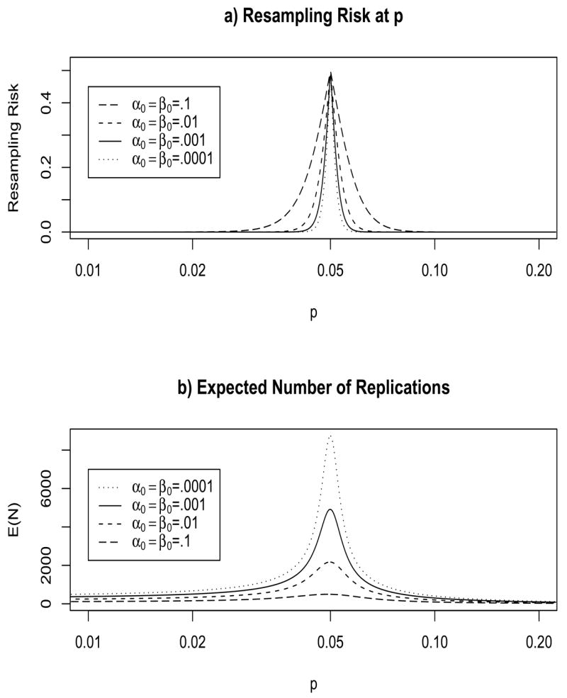
Properties of SPRT with p_a = .04 and p₀ = .0614 (so that C₀ = .05) using the Wald boundaries with α₀ and β₀ both equal to either 0.1, 0.01, 0.001 or 0.0001 (this corresponds to the parametrizations with C₁ = −C₂ equal to either 4.862, 10.168, 15.283 or 20.380 respectively). Figure 3a is resampling risk and Figure 3b is E(N), where both are calculated using Wald’s (1947) approximations.

6.2 Using a Truncated SPRT

In practice, we use a predetermined maximum N, say m. A simple truncation would be to use a SPRT except stop when N = m. We create a slight modification of this truncation by stopping at the curtailed boundary associated with m. In other words, we stop as soon as we either cross the SPRT boundary or the boundary with S_N ≥ α(m + 1) or N − S_N ≥ (1 − α)(m + 1). In this paper we will only explore this second type of truncated SPRT (or tSPRT). The details of the algorithm used to calculate the K_j values are given in the Appendix.

In Figures 4 we plot RR.₀₅(p) by p and E(N|p) by p for the fixed boundary with m = 9999 and several truncated SPRT boundaries with m = 9999, p_a = .04, and p₀ = 0.0614 (giving C₀ = .05). These calculations are based on using valid p-values as described in Section 5 and both RR.₀₅(p) and E(N|p) are exact, calculated using the K_j values from the algorithm in the Appendix. We see that the fixed boundary has the lowest resampling risk and the highest E(N). Notice we have a similar tradeoff as with the SPRT boundaries, as α₀ and β₀ get smaller the boundary widens (i.e., imagining the tSPRT boundary as a pencil shape [see Figure 2], the thickness of the pencil increases as α₀ and β₀ get smaller) and the resampling risk decreases while the E(N) increases. Note that RR.₀₅(p) can be larger than .5 and slightly asymmetrical; this is due to discreteness and the slightly conservative nature of the valid p-values, p̂_v.

Figure 4.

Properties of truncated SPRT with m = 9999, p_a = .04 and p₀ = .0614 (so that C₀ = .05) using the Wald boundaries with α₀ and β₀ both equal to either 0.1, 0.01, 0.001, or 0.0001 (this corresponds to the parametrizations with C₁ = − C₂ equal to either 4.862, 10.168, 15.283 or 20.380 respectively). Figure 4a is RR.₀₅(p) and Figure 4b is E(N), where both are calculated exactly using the algorithm in the appendix.

In the above we have held m constant, but we can also increase m, which will decrease the resampling risk and increase the E(N). But recall from Figure 3a that even with infinite m (i.e., a SPRT), the decrease in resampling risk is slight when going from α₀ = β₀ = .001 to α₀ = β₀ = .0001, so we expect that further reductions in α₀ and β₀ will not result in much reduction in RR_α per added E(N). Thus, we recommended the tSPRT boundary with α₀ = β₀ = .0001 and m = 9999 as a practical boundary for testing α = .05. In Figure 5 we show for this recommended boundary how the confidence intervals for the p-values are tightest close to p̂_v = 0.05.

Figure 5.

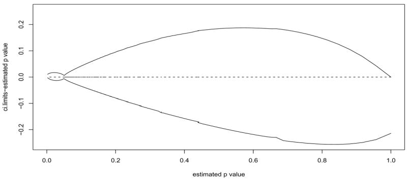
Plot of p̂_v vs. each of the 99% confidence limits minus p̂_v for the default tSPRT boundary with m = 9999, p_a = .04 and p₀ = .0614 (so that C₀ = .05) using the Wald boundaries with α₀ = β₀ = .0001.

7 Are the Simple P-value Estimators Valid?

We have already shown the p̂_MLE is not valid for any finite boundary. Since we have the software and algorithm to calculate the K_j values, we can calculate p̂_v; we can then try to find simple estimators of p similar to (4) and (5) that are valid.

Consider the tSPRT with m = 9999, p_a = 0.0400, p₀ = .0614, and α₀ = β₀ = .0001. This is equivalent to the tSPRT with m = 9999 and either p_a = 0.0466, p₀ = .0535 and α₀ = β₀ = .05; or p_a = 0.0490, p₀ = .0510 and α₀ = β₀ = .3. We consider two simple estimators, p̂_MLE(S_N, N) = S_N =N and p̃(S_N, N) = (S_N + 1)/(N + 1). In Figure 6a we plot p̂_MLE − p̂_v vs. p̂_v, and in Figure 6b we plot p̃ − p̂_v vs. p̂_v. We see that since both simple estimators drop below p̂_v for low p-values, and since for low p-values all three estimators have the same ordering, following the argument in Section 5, p̂ and p̃ are not valid. Notice that p̃ is closer to p̂_v for small p̂_v while p̂_MLE is closer to p̂_v for larger p̂_v. This is similar to the boundary of Besag and Clifford (1991) which has p̂_v equal to p̂_MLE for larger p-values and p̃ for smaller p-values.

Figure 6.

Validity of simple p-value estimators for the truncated SPRT with m = 9999, p_a = .04 and p₀ = .0614 with α₀ = β₀ = .0001. Figure 6a shows S_N =N − p̂_v vs. p̂_v, and Figure 6b shows (S_N + 1)/(N + 1) − p̂_v vs. p̂_v. Figure 6c shows p̂_A − p̂_v vs. p̂_v, where p̂_A is defined by (9). In both Figures 6a and 6b the difference falls below the line at 0, while in Figure 6c the difference never falls below 0, therefore, p̂_A is the only valid p-value of the three.

We propose a simple ad hoc estimator for p-values from this tSPRT boundary. Let

$${\widehat{p}}_A=\{\begin{array}{cc}\frac{S_N(1+\alpha /2)+1}{N+1}& \text{if }(S_N-C_2)/N\le \alpha \\ .04997& \text{if }N-S_N=max({\text{N}}_j-S_j)\\ \frac{S_N+1}{N+1}& \text{if }{S}_N=max({\text{S}}_j)\text{and}(S_N-C_1)/N<\alpha \\ \frac{S_N}{N}& \text{if }(S_N-C_1)/N\ge \alpha \end{array}$$ (9)

For the boundary of Figure 6c, p̂_A is valid since we can check every point in the boundary and show that p̂_A > p̂_v. For example, when N − S_N = max(N_j − S_j) then p̂_v(S_N, N) ∈ (.04910, .04997), so defining all p̂_A values as .04997 for those (S_N, N) values produces valid p-values. The utility of p̂_A is that it may be calculated without first calculating the K_j values. Note that p̂_A produces a valid p-value for only this one tSPRT boundary. It is an unsolved problem to define simple valid p-values for all tSPRT boundaries, although, as previously described, valid p-values may be calculated using the algorithm of the Appendix.

8 Application and Timings

Before applying the MC test with the tSPRT boundary to example data sets, there is some computation time that is required to set up the boundary. For example, on a personal computer with a Xeon 3.00GHz CPU with 3.5 GB of RAM, it took 73 minutes to calculate the tSPRT boundary with m = 9999, p_a = .04, p₀ = .0614, and α₀ = β₀ = .0001. This includes the time it took to calculate the 99% confidence intervals for each p-value. We call this boundary the default tSPRT boundary. Note, once that boundary is created and saved, then we can save computational time on a specific application of a MC test.

Now consider the application which motivated this research. Kim, et al (2000) developed a permutation test to see if there are significant changes in trend in cancer rates. Here we present the most basic application of the method. Figure 7 presents the standardized cancer incidence rates for all races and both sexes on a subset of the U.S. for either (a) brain and other nervous system cancer, (b) bones and joints cancer, or (c) eye and orbit cancer (SEER, 2006). For each type of cancer we plot a linear model, and the best joinpoint model (also called segmented line regression, or piecewise linear regression) with one joinpoint and joins allowed only on the years. We wish to test whether the joinpoint model fits significantly better than the linear model. To do this we perform an MC test, where the T₀ and T₁, T₂, … are defined as follows:

Figure 7.

Cancer incidence rates, standardized using the US 2000 standard (SEER, 2006). Solid line is the best linear fit and dotted line is the best 1-joinpoint fit, with joins allowed only exactly at each year.

1. Start with the observed data, letting d = d₀.

2. Calculate T(d) as follows:

   • Fit the linear regression model on d.

   • Do a grid search for the best joinpoint regression model on d with one joinpoint in terms of minimizing the sum of squares error (SSE), where joins are allowed only at the years (1976,1977,…,2002).

   • Calculate the statistic, T(d) equal to the SSE for the linear model over the SSE for the best joinpoint model on d.

3. Sequentially create permutation data sets by taking the predicted rates from the linear model on d₀, and adding the permuted residuals from the linear model also from d₀. Let these permutation data sets be denoted d₁, d₂, ….

4. Sequentially calculate T(d₁), T(d₂), … following Step 2.

Notice that this MC test requires a grid search for each permutation.

When we apply the MC test on the brain and other nervous system cancer rates using a fixed MC boundary with m = 9999 we get a p-value of p = 0.0001 with 99% confidence intervals on the p-value (0.00000, 0.00053). This took 24.6 minutes on the computer described above programmed in R. For this example, no attempt was made to optimize the computer code, since the timings will only be used to relatively compare the fixed boundary to the tSPRT boundary, and faster code, written in C++ with a graphical user interface, is freely available (Joinpoint, 2005). For the default tSPRT boundary, using the same random seed we get a p-value of p = 0.00244 with 99% confidence intervals on the p-value (0.00000, 0.01290). This took 1.0 minutes on the same computer (using precalculated K_j values and confidence intervals). Now apply the MC test on the bones and joints cancer rates. For the fixed MC boundary with m = 9999, we get a p-value of p = 0.308 with 99% confidence intervals on the p-value (0.296, 0.320), and it takes 24.6 minutes. For the default tSPRT boundary, using the same random seed we get a p-value of p = 0.369 with 99% confidence intervals on the p-value (0.222, 0.528). This took 9.8 seconds on the same computer. Applying the MC test on the eye and orbit cancer, it took 24.7 minutes to get a p-value of p = .0555 with 99% confidence intervals (0.0497, 0.0616) using the fixed MC boundary with m = 9999, and it took 3.6 minutes to get a p-value of 0.0634 with 99% confidence interval (0.0475, 0.0814) using the default tSPRT boundary. In all cases using the tSPRT boundary resulted in a savings in terms of time (not counting the set-up time) at the cost of precision on the p-value. In the third example there was less savings in time because the p-value was closer to 0.05.

The advantage of the tSPRT boundary over the fixed type boundary is apparent when each application of the test statistic is not trivially short. Then the tSPRT boundary automatically adjusts to take few replications when the p-value is far from α giving fairly large confidence intervals on the p-value, but takes many replications when the p-value is close to α giving relatively tight confidence intervals. Thus, for example, the tSPRT boundary is very practical for applying the joinpoint tests repeatedly to many different types of cancer rates.

9 Discussion

We have explored the use of truncated sequential probability ratio test (tSPRT) boundaries with MC tests. We related the p-value from an MC test to some classical results on sequentially testing of a binomial parameter, and provided an algorithm useful for calculating many of those results. Using that algorithm, we have shown how to calculate valid p-values and confidence intervals about those p-values. We have shown the form of a minimax SPRT boundary with respect to the resampling risk for α (RR_α). Among that class of minimax boundaries, we have shown (at least with resample sizes around 10⁴ for α = 0.05) that a reasonable tSPRT uses p_a = 0.04 and α₀ = β₀ = 0.0001 for the Wald parameters. Other reasonable tSPRT boundaries may have α₀ ≠ β₀, and we leave the exploration of the relative size of those parameters for future research.

There are other methods that may be used to decide among the tSPRT boundaries from within the minimax class even with α₀ = β₀ (or equivalently (C₁ = −C₂). Here we mention three. First one could choose C₁ = −C₂ such that the minimum possible p-value is less than some value, p_min. Note that the minimum p-value for the tSPRT boundary occurs when S_j = 0. Let that point be (S_b = 0, N_b). Then p̂_v(0, N_b) = 1/(N_b + 1) and N_b = [−C₂/α], where [x] is the smallest integer greater than or equal to x. For the default tSPRT (i.e., with parameters m = 9999, p_a = .04, p₀ = .0614, and α₀ = β₀ = .0001) we have that N_b = 408 and the minimum p-value is p = 0.0024.

A second method for choosing tSPRT parameters was suggested by the associate editor. Let m_f be the resample size for a fixed boundary that gives an acceptable width confidence interval at p̂ = .05. Set m for the tSPRT boundary at some multiple of m_f, say m = 1.5m_f, then solve for α₀ = β₀ so that the tSPRT confidence interval at p̂ = .05 has approximately the same width as the fixed boundary with m_f.

Finally, another way to choose an MC boundary, is to minimize the resampling risk among a set of distributions for the p-value as proposed by Fay and Follmann (2002). We briefly outline that approach, which adds an extra level of abstraction. Note from Figure 4a that the resampling risk varies widely throughout p. It would be nice to summarize RR_α(p) by taking the mean over all p. To do this we assume a distribution for the p-value. Let P be a random variable for the p-value, whose distribution is induced by the test statistic and the data. Define the random variable Z = g {T(D₀)}, where D₀ is a random variable representing the original data, and g(·) is an unknown monotonic function. Note that Z is a random variable, whose randomness comes from the data, while in much of paper, the original data, d₀, was treated as fixed and the only randomness came from the Monte Carlo resamplings. Suppose there exists some g(·) (possibly the identity function) such that under the null Z ~N(0, 1) and under the alternative Z ~N(μ, 1). We can rewrite μ in terms of α and the power of the test, 1 − β, as μ = Φ⁻¹(1 − α) − Φ⁻¹(β). Because of the central limit theorem many common test statistics induce random variables Z of this form. Then the distribution of the p-value under the alternative is F_P (x; μ) = 1 − Φ {Φ⁻¹(1 − x) − μ}. Fay and Follmann (2002) defined the resampling risk in terms of distributions for P as RR_α(F_P) = ∫RR_α(p)dF_P (p). They estimated F_P with beta distributions, F̂_P, then looked for the F̂_P which gave the largest RR_α(F̂_P) for fixed boundaries of different sizes over all possible values of β. They found through a numeric search that 1 − β equal to about .47 gave the largest RR_0.05(F̂_P) for fixed boundaries. We have found through numeric search that 1 − β = .47 also gave the largest RR_α(F̂_P) for fixed boundaries when α = 0.01. Let the distribution associated with 1 − β = .47 be F̂*. Thus, another method for choosing tSPRT would be to choose a maximum allowable RR_α(F̂*), say γ, then either (1) fix a suitable α₀ and β₀ and increase m until RR_α(F̂*) < γ, or (2) fix a suitable m and decrease α₀ = β₀ until RR_α(F̂*) < γ. The term suitable applied to the fixed parameters above denotes that RR_α(F̂*) < γ is possible by changing the other parameter(s). Note that RR_α(F̂*) = 0.0041 for the recommended tSPRT boundary with m = 9999; p₀ = .04, p₁ = 0.0614, and α₀ = β₀ = 0.0001.

We have not discussed other classes of boundaries such as the IPO boundary recommended by Fay and Follmann (2002) for bounding RR_α(F̂*). We simply note that the IPO boundary is intractable for values of RR_α(F̂*) smaller than 0.01, and in cases we studied where it is tractable, the IPO performs similarly to tSPRT boundaries (results not shown).

Note that there have recently been many advances in group sequential methods especially for use in monitoring clinical trials (see Jennison and Turnbull, 2000, and Proschan, Lan, and Wittes, 2006). We briefly show how these methods relate to the truncated SPRT. For group sequential methods, we specify a sample size for the certain end of the trial then specify either (1) how many looks at the data will be taken and which monitoring procedure will be used or (2) how the type I error will be spent by picking a spending function. To study both approaches for the MC test situation we first write the tSPRT as a B-value (Lan and Wittes, 1988). Suppose that we specify that the trial will continue until at most m observations and each observation is binary. Let Z_m be the statistic for testing whether p = α or not given a sampling of m observations:

$$Z_m=\frac{S_m-m\alpha }{\sqrt{m\alpha (1-\alpha )}}$$

Similarly we can define Z_N after N observations. At the N th observation, we are $\sqrt{N/m}$ of the way through the trial in terms of information. The B-value at the trial fraction $t=\sqrt{N/m}$ is,

$$B\left(\sqrt{\frac{N}{m}}\right)=\sqrt{\frac{N}{m}}{Z}_N=\frac{S_N-N_{\alpha }}{\sqrt{m\alpha (1-\alpha )}}$$

If we are taking an fixed number of equidistant looks at the data, at say $t_1=\sqrt{n_1/m},t_2=\sqrt{n_2/m},\dots t_k=1$, then using the standard recommended O’Brien-Fleming procedure we stop before t_k = 1 if either $B(t_i)\ge C_1^{\ast }$ or $B(t_i)\le C_2^{\ast }$ for any i < k, or equivalently at n_i = N < m stop if

$$S_N\ge C_1^{\ast }\sqrt{m\alpha (1-\alpha )}+N\alpha$$

or if

$$S_N\le C_2^{\ast }\sqrt{m\alpha (1-\alpha )}+N\alpha .$$

With m looks at the data we get the tSPRT minimax boundary that we have proposed. There has been some work on optimizing the group sequential methods (see Jennison and Turnbull, 2000, p. 357–359 and references there), but the added complexity does not seem worthwhile for MC tests where we allow stopping after each replicate. The spending function approach mentioned above just adds more flexibility so that the looks do not need to be at predetermined times. Unlike a clinical trial were it is logistically difficult to perform many analyses on the data as the trial progresses, there is very little extra cost in checking after each observation for an MC test.

Finally, we note that the algorithm listed in the Appendix may be used for calculating exact confidence intervals following a tSPRT for a binary response. The estimator of p in this case need not be p̂_v, and an appropriate estimator may be either the MLE or the unbiased estimator (which also uses the algorithm of the Appendix in its calculation).

An R package called MChtest to perform the methods of this paper is available at CRAN (http://cran.r-project.org/).

Appendix: Algorithm for Calculating K_j

Here we present an algorithm for calculating the number of ways to reach the jth boundary point, K_j, for a tSPRT design. Modifications to the algorithm may be needed to apply it to different designs and are not discussed here.

First we define the ordering of the indices of the design. Let R_j = N_j − S_j for all j. The first point in the design has S₁ = N₁ and R₁ = 0. The next set of points has R₂ = 1, R₃ = 2, … but including only those points with S_j/N_j > α. At S_j/N_j = α we order the points by decreasing values of S_j until we reach the last point at S_b = 0. In the following let the rows from i to j of B be denoted B_[i:j].

Now here is the algorithm:

• Start with the smallest curtailed sampling design (see e.g., Fay and Follmann, 2002) that is surrounded by the proposed design B. In other words each point on the curtailed sampling design is either a member of the proposed boundary, B, or it is on the interior of B. Let B⁽¹⁾ denote this curtailed design. Let R_j = N_j − S_j for all j, and similarly define ${\text{R}}_j^{(k)}$. Because it is a curtailed design, every point in this design has either ${\text{S}}_j^{(1)}={max}_i({\text{S}}_i^{(1)})$ (the “top” of the design) or ${\text{R}}_j^{(1)}={max}_i({\text{R}}_i^{(1)})$ (the “right” of the design). Then for each point, (s, n), on the top of this curtailed design the K-value is $K(s,n)=\left(\begin{array}{c}n-1\\ n-s\end{array}\right)$. For each point, (s; n), on the right of the design the K-value is $\left(\begin{array}{c}n-1\\ s\end{array}\right)$.

• Keep iterating from B^(j) to B^(j+1) until B^(j+1) = B. Within the iterations we define 3 indexes, i₁ ≤ i₂ ≤ i₃. The index $i_1=i_1^{(j)}$ is the largest index i such that ${\mathit{B}}_{[1:i]}^{(j)}={\mathit{B}}_{[1:i]}$. The index $i_2=i_2^{(j)}$ is the top index for B^(j), i.e., i₂ is the smallest value of i such that ${\text{S}}_{i+1}^{(j)}<{\text{S}}_i^{(j)}$. The index $i_3=i_3^{(j)}$ is the smallest index that i such that ${\mathit{B}}_{[i:s^{(j)}]}^{(j)}={\mathit{B}}_{[(s-s^{(j)}+i):s]}$, where s is the number of rows in B and s^(j) is the number of rows in B^(j). This means that there are s^(j) − i₃ + 1 rows that match at the end of B^(j) and B.

  1. Keep moving up the top row until all of the top of B^(j+1) equals the beginning of the top of B, then go to 2. To move up the top row, do the following:

     • – Start from the design B^(j) with corresponding count vector denoted K^(j).

       Let

       $${\mathit{B}}_{[1:i_1]}^{(j+1)}={\mathit{B}}_{[1:i_1]}^{(j)}$$

       $$\begin{array}{l}{\mathit{B}}_{[(i_1+1):i_2]}^{(j+1)}=\left[\begin{array}{cc}{\text{S}}_{i_1+1}^{(j)}+1& {\text{N}}_{i_1+1}^{(j)}+1\\ {\text{S}}_{i_1+2}^{(j)}+1& {\text{N}}_{i_1+2}^{(j)}+1\\ ⋮& ⋮\\ {\text{S}}_{i_2}^{(j)}+1& {\text{N}}_{i_2}^{(j)}+1\end{array}\right]\\ {\mathit{B}}_{i_2+1}^{(j+1)}=\left[\begin{array}{cc}{\text{S}}_{i_2}^{(j)}& {\text{N}}_{i_2}^{(j)}+1\end{array}\right]\end{array}$$

       and
       $${\mathit{B}}_{[(i_2+2):(s^{(j)}+1)]}^{(j+1)}={\mathit{B}}_{[(i_2+1):s^{(j)}]}^{(j)}$$

       Then K^(j+1) is equal to

       $$\begin{array}{l}{\mathit{K}}_{[1:i_1]}^{(j+1)}={\mathit{K}}_{[1:i_1]}^{(j)}\\ {\mathit{K}}_{[i_1:i_2]}^{(j+1)}=\left[\begin{array}{c}{K}_{i_1}^{(j)}\\ {\sum }_{i=i_1}^{i_1+1}{K}_i^{(j)}\\ ⋮\\ {\sum }_{i=i_1}^{i_2}{K}_i^{(j)}\end{array}\right]\\ {\mathit{K}}_{[(i_2+1):(i_2+1)]}^{(j+1)}=\left[\sum _{i=i_1}^{i_2}{K}_i^{(j)}\right]\\ {\mathit{K}}_{[(i_2+2):(s^{(j)}+1)]}^{(j+1)}={\mathit{K}}_{[(i_2+1):s^{(j)}]}^{(j)}\end{array}$$

  2. Keep moving right the right hand-side of the design until all of the right of B^(j+1) equals the end of the right of B, if B^(j+1) ≠ B go to 1. To move over the right of the design, do the following:

     • – Start from the design B^(j) with corresponding count vector denoted K^(j). We want to move the portion of the right hand side of B^(j) that is not already equal (i.e., ${\mathit{B}}_{[(i_2+1):(i_3-1)]}^{(j)}$) over 1 position to the right. Then

       $$\begin{array}{l}{\mathit{B}}_{[1:i_2]}^{(j+1)}={\mathit{B}}_{[1:i_2]}^{(j)}\\ {\mathit{B}}_{[(i_2+1):(i_2+1)]}^{(j+1)}=\left[\begin{array}{cc}{\text{S}}_{i_2}^{(j)}& {\text{N}}_{i_2}^{(j)}+1\end{array}\right]\\ {\mathit{B}}_{[(i_2+2):i_3]}^{(j+1)}=\left[\begin{array}{cc}{\text{S}}_{i_2+1}^{(j)}& {\text{N}}_{i_2+1}^{(j)}+1\\ {\text{S}}_{i_2+2}^{(j)}& {\text{N}}_{i_2+2}^{(j)}+1\\ ⋮& ⋮\\ {\text{S}}_{i_3-1}^{(j)}& {\text{N}}_{i_3-1}^{(j)}+1\end{array}\right]\end{array}$$

       and
       $${\mathit{B}}_{[(i_3+1):(s^{(j)}+1)]}^{(j+1)}={\mathit{B}}_{[i_3:s^{(j)}]}^{(j)}$$

       Then K^(j+1) is

       $$\begin{array}{l}{\mathit{K}}_{[1:i_2]}^{(j+1)}={\mathit{K}}_{[1:i_2]}^{(j)}\\ {\mathit{K}}_{[(i_2+1):(i_2+1)]}^{(j+1)}=\left[\sum _{i=i_2+1}^{i_3-1}{K}_i^{(j)}\right]\\ {\mathit{K}}_{[(i_2+2):i_3]}^{(j+1)}=\left[\begin{array}{c}{\sum }_{i=i_2+1}^{i_3-1}{K}_i^{(j)}\\ {\sum }_{i=i_2+2}^{i_3-1}{K}_i^{(j)}\\ ⋮\\ {\sum }_{i=i_3-1}^{i_3-1}{K}_i^{(j)}\end{array}\right]\end{array}$$

       and
       $${\mathit{K}}_{[(i_3+1):(s^{(j)}+1)]}^{(j+1)}={\mathit{K}}_{[i_3:s^{(j)}]}^{(j)}$$

       To avoid overflow, we do not store the K_j values, but instead store

       $$K_j^{\ast }=K_j\beta ({\text{S}}_j+1,{\text{R}}_j+1).$$

References

- Agresti A. A survey of exact inference for contingency tables. Statistical Science. 1992;7:131–177. [Google Scholar]
- Armitage P. Numerical studies in the sequential estimation of a binomial parameter. Biometrika. 1958;5:1–15. [Google Scholar]
- Berger RL, Boos DD. P values maximized over a confidence set for the nuisance parameter. Journal of the American Statistical Association. 1994;9:1012–1016. [Google Scholar]
- Besag J, Clifford P. Sequential Monte Carlo p-values. Biometrika. 1991;78:301–304. [Google Scholar]
- Efron B, Tibshirani RJ. An Introduction to the Bootstrap. Chapman and Hall; New York: 1993. [Google Scholar]
- Eisenberg B, Ghosh BK. The Sequential Probability Ratio Test. In: Ghosh BK, Sen PK, editors. Handbook of Sequential Analysis. Chapter 3. Marcel Dekker, Inc.; New York: 1991. [Google Scholar]
- Fay MP, Follmann DA. Designing Monte Carlo implementations of permutation or bootstrap hypothesis tests. American Statistician. 2002;56:63–70. [Google Scholar]
- Girshick MA, Mosteller F, Savage LJ. Unbiased estimates for certain binomial sampling problems with applications. Annals of Mathematical Statistics. 1946;17:13–23. [Google Scholar]
- Gleser LJ. Comment on “Bootstrap Confidence Intervals” by T.J DiCiccio and B Efron. Statistical Science. 1996;11:219–221. [Google Scholar]
- Jennison C, Turnbull BW. Group Sequential Methods with Applications to Clinical Trials. New York: Chapman and Hall/CRC; 2000. [Google Scholar]
- Statistical Research and Applications Branch, National Cancer Institute. Joinpoint Regression Program, Version 3.0. 2005 April; ( http://srab.cancer.gov/joinpoint/)
- KimH-JFay MP, Feuer EJ, Midthune DN. Permutation tests for join-point regression with applications to cancer rates. Statistics in Medicine. 2000;9:335–351. doi: 10.1002/(sici)1097-0258(20000215)19:3<335::aid-sim336>3.0.co;2-z. (correction: 2001 20, 655) [DOI] [PubMed] [Google Scholar]
- Lan KKG, DeMets DL. Discrete sequential boundaries for clinical trials. Biometrika. 1983;70:659–663. [Google Scholar]
- Lan KKG, Wittes J. The B-Value: A tool for monitoring data. Biometrics. 1988;44:579–585. [PubMed] [Google Scholar]
- Lehmann EL. Theory of Point Estimation. New York: Wiley; 1983. [Google Scholar]
- Lock RH. A Sequential Approximation to a Permutation Test. Communications in Statistics: Simulation and Computation. 1991;20:341–363. [Google Scholar]
- Mehta CR, Patel NR, Senchaudhuri P. Importance sampling for estimating exact probabilities in permutational inference. Journal of the American Statistical Association. 1988;83:999–1005. [Google Scholar]
- Proschan MA, Lan KKG, Wittes JT. Statistical Monitoring of Clinical Trials: A Unified Approach. New York: Springer; 2006. [Google Scholar]
- Schultz JR, Nichol FR, Elfring GL, Weed SD. Multi-stage procedures for drug screening. Biometrics. 1973;29:293–300. [PubMed] [Google Scholar]
- SEER. Surveillance, Epidemiology, and End Results Program. 2006 ( www.seer.cancer.gov) SEER*Stat Database: Incidence - SEER 9 Regs Public-Use, Nov 2005 Sub (1973–2003), National Cancer Institute, DCCPS, Surveillance Research Program, Cancer Statistics Branch, released April 2006, based on the November 2005 submission.
- Siegmund D. Sequential Analysis. New York: Springer-Verlag; 1985. [Google Scholar]
- Wald A. Sequential Analysis. New York: Dover; 1947. [Google Scholar]