From snapshot to movie: φ analysis of protein folding transition states taken one step further

Abstract

Kinetic anomalies in protein folding can result from changes of the kinetic ground states (D, I, and N), changes of the protein folding transition state, or both. The 102-residue protein U1A has a symmetrically curved chevron plot which seems to result mainly from changes of the transition state. At low concentrations of denaturant the transition state occurs early in the folding reaction, whereas at high denaturant concentration it moves close to the native structure. In this study we use this movement to follow continuously the formation and growth of U1A's folding nucleus by φ analysis. Although U1A's transition state structure is generally delocalized and displays a typical nucleation–condensation pattern, we can still resolve a sequence of folding events. However, these events are sufficiently coupled to start almost simultaneously throughout the transition state structure.

In the quest to understand how proteins fold, an increasing number of studies have been focused on structural characterization of the transition state ensemble—the kinetic bottleneck for folding (1–3). The results provide fascinating snapshots of the high-energy conformational states that have greatly improved our view of how proteins adopt their structure. Interestingly, it emerges that small two-state proteins do not fold in a strictly hierarchical manner but establish their interactions more or less simultaneously within a diffuse and global nucleus (4). An irresistible challenge now is to refine the details of this process. How does the nucleus form and consolidate? What gives rise to different nucleation patterns? Is there a single obligate nucleus (5), or could multiple nuclei act in concert (6)?

As the transition state (‡) never accumulates, details about its structure have been inferred indirectly from the folding rate and protein engineering (7). By systematically truncating side chains while probing the effects on the kinetics, it is possible to map out detailed interaction patterns in ‡. In effect, mutations that destabilize ‡ are said to target contacts in its structure. The strength of the contacts is measured by the phi value (φ^‡), which normalizes the stability loss of ‡ to that of the native protein. φ^‡ = 1 indicates that the site of mutation is fully structured in the transition state, whereas φ^‡ = 0 indicates that the site is unfolded. The first two-state protein to be characterized by this method was CI2 (8). The results revealed a new type of folding behavior, apparently inconsistent with earlier hierarchical models developed from studies of larger multistate proteins (9). CI2's ‡ shows a global distribution of fractional φ^‡s diffusely centred on three residues with high φ^‡s in the hydrophobic core (8). The result suggests a large and delocalized nucleus where secondary and tertiary structure condenses concomitantly around a leading density in its center. The behavior was denoted nucleation condensation (4). Similar, delocalized nuclei of fractional φ^‡s have later been observed for Arc repressor (10), CheY (11), and λ repressor (12). But there is some variation in the nucleation patterns. With the homologous and all-β structure SH3 domains from src (13) and α-spectrin (14), it is evident that one end of the protein forms earlier than the rest, giving rise to “polarized” ‡ structures with distinguishable interfaces between ordered and disordered regions.

In this study we explore a different strategy to investigate further the delocalized nucleation process: we scan the folding events with a moving transition state by tuning the protein stability. This procedure allows us to follow continuously the development and consolidation of the folding nucleus of the two-state protein U1A (15). Despite U1A's delocalized nucleation pattern, a clear but somewhat overlapping sequence of folding events is resolved. The first ordered interactions appear between strands 2 and 3 and helix 1, forming part of the hydrophobic core. Subsequently, strand 1 wraps around the still-expanded half-core and, finally, the structure is closed up by the condensation of strand 4 and helix 2. The latter event could be interpreted either as a protrusion of the main nucleus or as a secondary nucleation event. Notably, the folding events are so tightly coupled that they start almost simultaneously throughout the protein, thus causing the transition state structure to appear overall diffuse.

Materials and Methods

Materials.

Mutagenesis was done by standard procedures using the Quick-Change kit (Stratagene). Expression and purification of protein was done as in ref. 15. Buffer was 50 mM Mes at pH 6.3 (19 mM acid and 31 mM salt). Guanidinium chloride (GdmCl) was ultrapure from GIBCO/Life Technologies. All stopped-flow analysis was done at 298 K on a SX 18 MV instrument from Applied Photophysics (Surrey, U.K.), and curve fitting was done with the KaleidaGraph software (Abelbeck Software, Reading, PA). For experimental procedures see Results.

NMR.

The ¹⁵N-labeled samples contained 1.0–1.2 mM protein dissolved in 600 μl of 5 mM sodium acetate buffer (90% H₂O/10% D₂O) at pH 4.8/50 mM NaCl/80 μM 2,2-dimethyl-2-silapentane-5-sulfonate (DSS). Experiments were done on 500- and 600-MHz Varian UNITY Inova spectrometers at ¹H Larmor frequencies of 499.78 and 599.89 MHz, respectively. A three-dimensional ¹⁵N total correlation spectroscopy–heteronuclear single quantum correlation (TOCSY–HSQC) experiment (16) using DIPSI-rc mixing (17, 18) was acquired at 600 MHz with spectral widths of 6601 Hz in ω₁ and ω₃, and 1860 Hz in ω₂, sampled over 128, 1024, and 48 complex points, respectively. ¹⁵N–¹H HSQC (19) spectra were acquired by using sensitivity-enhanced pulsed field gradient coherence selection (20–22) and GARP-1 (23) ¹⁵N decoupling during acquisition. The sample was dissolved in ice-cold D₂O and immediately placed at 303 K in the spectrometer, which had been tuned and calibrated with a sample of identical composition. Processing and analysis of the spectra were by Felix97 (MSI, San Diego). ¹⁵N–¹H HSQC spectra were processed with exponential and cosine apodization functions in ω₂ and ω₁, respectively. Final size of the matrix was typically 2048 × 256 real points after zero-filling and Fourier transformation. Crosspeak intensities were evaluated as peak heights and decays were evaluated by standard procedures (24).

Results

Curved Chevron Plots and Transition State Movements.

The gross appearance of the transition state (‡) is often inferred from mass action—i.e., from the GdmCl dependence of the activation process for refolding (D ⇌ ‡) and unfolding (N ⇌ ‡). The GdmCl response is measured by the kinetic m values

1

where k_u and k_f are the unfolding and refolding rate constants, respectively. Often, the m values are constants, implying a proportionality between m values and changes in the protein's solvent-accessible surface area (25). This proportionality is also evident from the good agreement between m values and changes in heat capacity (26, 27). For two-state folding where K_D-N = k_u/k_f and consequently

2

It is thus possible to assign the position of ‡ in relation to D and N according to

3

where β^‡ is a normalized measure of how the stability of ‡ changes upon addition of denaturant (25, 28). A more structural interpretation of β^‡ is the solvent exposure of ‡ relative to that of N. Consistently, β^‡ may also be inferred from transient heat capacity changes (27) and transient pK_a shifts (29).

Experimentally, folding kinetics are evaluated from so-called chevron plots (log k vs. [GdmCl]) (Fig. 1). For two-state proteins these are characteristically V-shaped with fixed values of m_f, m_u, and β^‡ (3, 30). For U1A, however, the chevron plot is symetrically curved, showing that the m values vary with [GdmCl]; m_f grows larger while m_u decreases (Fig. 1). Notably, the increase in m_f is precisely coupled to the decrease in m_u, maintaining a constant value of m_D-N (Eq. 2). This suggests that U1A displays two-state kinetics at all [GdmCl], and that the curvatures result from changes in β^‡. That is, the curvature results from changes of U1A's transition state; at high concentrations of GdmCl, ‡ moves closer to N, resulting in a smaller structural change upon activation N ⇌ ‡ and thus a lower value of m_u (31). A measure of the ‡ movement is given by Eq. 3, and β^‡ ranges from ∼0.2 at 0.45 M GdmCl to ∼0.9 at 8 M GdmCl (Fig. 1). Analogous movements have been observed for barnase (32), Arc repressor (10), and CI2 (33) and have recently been induced by mutations in CI2 and S6 (34). The behavior is also suggested by theory and simulations in which the kinetic bottleneck changes location in the folding funnel upon changing of the stability (35).

Figure 1.

The symmetrically curved chevron plot of U1A reveals a progressive change of the kinetic m values. The phenomenon is here ascribed to transition state movements along β̂ (Eqs. 1–3). Data below 1.5 M GdmCl were excluded from the fits to eliminate problems with transient aggregation (▾).

An alternative explanation for curved unfolding limbs would be that strong GdmCl solutions are not ideal (25, 36). Although plots of log k_u vs. GdmCl activity yield reasonably straight lines, they produce at the same time upward curvatures in proteins with V-shaped chevrons (34). Such upward curvatures are not easily rationalized by either ‡ movements or the existence of intermediates. Further, the curvature of U1A's unfolding limb is seen also with the noncharged denaturant urea (data not shown). A third explanation is unfolding intermediates (37)—i.e., the curvatures arise from partial disrupture of N prior to global unfolding (38). In the case of U1A, however, we disfavor this scenario also, because the structure in question shows high H/D protection factors (see below). Remember that identical curvature is seen also on the refolding side, which means that any unfolding intermediate needs to be accompanied by a symmetrically located refolding intermediate. Together with U1A's two-state characteristics, a moving transition state appears to be the simpler explanation. And perhaps most important: moving transition states provide an alternative and unexplored way of accounting for anomalous folding kinetics. For an extensive analysis of U1A's two-state behavior, including D- and N-like dead-time spectra and coinciding GdmCl titrations with CD and fluorescence, see ref. 39.

Construction of the Free-Energy Profile.

The movement of ‡ was used to reconstruct the shape of the folding free-energy profile as follows (30, 31, 33, 34) (Fig. 2).

Figure 2.

Derivation of barrier shape from chevron plot. Units are in s⁻¹ and 2.3RT. See steps 1–3 in Results. The broad and level barrier profile cause its highest point (‡) to move upon destabilization with GdmCl.

Step 1.

To account for the curvatures, log k_f and log k_u were fitted by second-order polynomials the derivatives of which yield the kinetic m values—i.e., m_f = b_f + 2c_f[GdmCl] and m_u = b_u + 2c_u[GdmCl] (Eq. 1, Table 1). β^‡ was then calculated from Eq. 3, where m_D-N was derived either kinetically from m_f and m_u (Eq. 2) or estimated independently from equilibrium unfolding, and the chevron data were replotted against β^‡ (Fig. 2). Data below 1.5 M GdmCl were excluded from the fits to eliminate perturbations from transient aggregation (40).

Table 1.

Parameters from curve fits to chevron data: log k_obs = log(k_f + k_u) = log(10^logk_f+ 10^logk_u), where k_obs is the observed rate constant, and log k_f and log k_u were replaced by second-order polynomials log k_f = a_f − b_f[GdmCl] − c_f[GdmCl]² and log k_u = a_u + b_u[GdmCl] − c_u[GdmCl]²

Mutation	Deleted contacts	MP	mD-N	ΔΔGD-N/ 2.3RT	af	bf	au	bu	cu = cf	φ
										β‡ = 0.3	β‡ = 0.5	β‡ = 0.7	β‡ = 0.85
Wild type		4.1	1.82	0	2.4  ±  0.0	−0.31  ±  0.02	−5.0  ±  0.1	1.51  ±  0.03	−0.08
I12V, β1	V57 β1, A65 α1	3.4	1.86	1.2	2.4  ±  0.0	−0.29  ±  0.03	−4.0  ±  0.1	1.56  ±  0.04	−0.09	0.0	0.1	0.25	0.4
I14A, β1	L17 β1	2.2	1.81	3.3	2.5  ±  0.1	−0.88  ±  0.06	−1.5  ±  0.0	0.93  ±  0.01	−0.06	—	0.35	0.6	0.75
L17A, β1	I14 β1, L26 α1	2.6	1.80	2.7	2.6  ±  0.1	−0.56  ±  0.04	−2.1  ±  0.1	1.24  ±  0.04	−0.09	—	0.2	0.45	0.65
L26A, α1	L17 β1, I21, L30 α1, Y78	3.1	1.69	1.7	2.0  ±  0.0	−0.38  ±  0.02	−3.3  ±  0.1	1.31  ±  0.04	−0.08	0.1	0.35	0.6	0.8
L30A, α1	L26 α1, K27 α1, I43 β2	2.0	1.81	3.8	2.2  ±  0.1	−0.95  ±  0.07	−1.3  ±  0.1	0.86  ±  0.03	−0.05	—	(0.4)	0.65	0.85
F34A, α1	L30, I33, V57 β3, M72 α2	2.1	1.55	3.3	2.3  ±  0.0	−0.89  ±  0.04	−1.0  ±  0.1	0.66  ±  0.04	−0.03	—	(0.4)	0.65	0.85
I40A, β2	F34 α1, S35 α1, I43 β2,	2.0	1.74	3.8	2.5  ±  0.1	−1.20  ±  0.07	−0.9  ±  0.0	0.54  ±  0.02	−0.03	—	(0.4)	0.75	0.95
	V57 β3, F59 β3
I43V, β2	Y31 α1	3.9	1.86	0.4	2.3  ±  0.0	−0.43  ±  0.03	−4.9  ±  0.1	1.43  ±  0.05	−0.08	1.0	1.2	1.3	1.5
V45A, β2	A55 β3	3.1	1.71	1.7	1.9  ±  0.0	−0.51  ±  0.03	−3.5  ±  0.1	1.20  ±  0.05	−0.07	0.35	0.6	0.9	1.1
I58A, β3	H10 β1, L44 β2, I94 α3	3.5	1.55	1.0	2.0  ±  0.0	−0.71  ±  0.03	−3.4  ±  0.1	0.84  ±  0.06	−0.03	—	—	—	—
L69A, α2	R70 α2, Q73, Q85 β4	3.1	1.56	1.7	2.8  ±  0.1	−0.62  ±  0.06	−2.0  ±  0.2	0.94  ±  0.08	−0.05	(<0)	0.0	0.5	0.7
I84V, β4	Q73	3.6	1.92	1.0	2.3  ±  0.1	−0.16  ±  0.06	−4.6  ±  0.3	1.76  ±  0.10	−0.11	<0	0.0	0.2	0.4
I84A, β4	I12 β1, A68 α2, Q73	2.7	1.40	2.2	2.4  ±  0.0	−0.37  ±  0.03	−1.4  ±  0.1	1.03  ±  0.03	−0.07	(<0)	<0	0.25	0.5

MP, GdmCl concentration (M) at the transition midpoint obtained from the intersection of the fitted polynomials; errors < ±0.04. m_D-N, Equilibrium m value derived from kinetic fits—i.e., b_f + b_u (Eqs. 1 and 2). ΔΔG_D-N/2.3RT = log K_D-N, stability loss upon mutation derived from kinetic fits at (MP_wt + MP_mut)/2, assuming two-state behavior K_D-N = k_u/k_f. c_u = c_f. Errors < ±0.01. φ, parentheses indicate that the values are slightly extrapolated—cf. graphs in Fig. 5. 

Step 2.

The barrier height (D ⇌ ‡) at each point of β^‡ was approximated as ΔG^‡ = 2.3RT (6 − log k_f), where the pre-factor of 10⁶ s⁻¹ is from ref. 41. In the unfolding region k_f was obtained from k_u and Eq. 3. Note that each point on this curve is obtained at a different [GdmCl]: early parts are linked to rate constants obtained at low [GdmCl] in the refolding region, whereas late parts are linked to high [GdmCl] in the unfolding region. A clearer representation of the free-energy profile is obtained if all points are extrapolated to a common [GdmCl]. This is done next by linear free-energy extrapolations.

Step 3.

As β^‡ is simply the normalized sensitivity to GdmCl (Eq. 3), each value of ΔG^‡ can be extrapolated to a common [GdmCl] (Y) by standard linear free-energy relations: ΔG^‡(β^‡, [Y]) = ΔG^‡(β^‡, [X]) + β^‡m_D-N 2.3RT([Y] − [X]), where [X] is the GdmCl concentration at which log k_f was measured. The bottom panels in Fig. 2 show the resulting free-energy profiles at 0, 4, and 8 M GdmCl, and illustrate how ‡ moves along the top of a broad barrier as [GdmCl] is increased. The key assumption behind the barrier construction is thus that folding proceeds by the same events at all [GdmCl]. Consistent motions of the transition state over broad barriers are predicted independently by theoretical models both in the mean-field and capillarity limit (42, 43). Note also that the broad barrier representation provides a simple rationale for Hammond postulate behavior in protein folding (30, 32).

From Snapshot to Movie.

Transition state movements open the possibility to continuously follow the development of interactions along β^‡. We do this by φ^‡ analysis at each point along the barrier top. To improve the resolution we constrained the system to ideal two-state behavior by the following measures, all of which fall within the experimental error: (i) the transition midpoint and m_D-N are derived kinetically, which yields higher precision than equilibrium measurements; (ii) the kinetic curvatures are assumed to be caused by ‡ changes alone; and (iii) on the basis of data where both limbs of the chevron plot are clearly resolved we have fixed the quadratic terms in the polynomial fits to the same value, i.e. c_f = c_u. Data for 10 typical mutants are shown in Fig. 3. Barrier profiles were obtained as for wild type.

Figure 3.

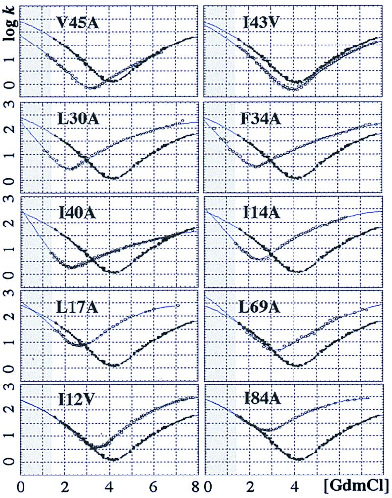
Chevron plots for the U1A mutants (○) superimposed on wild type data (●).

For calculation of φ vs. β^‡, the wild-type profile (ΔG^‡,wt (β^‡)) was subtracted from that of the mutant (ΔG^‡,mut (β^‡)) (Fig. 4), and the difference was divided by the destabilization of N upon mutation (ΔΔG_D-N)

4

which yields a φ^‡ at each point of β^‡ where the barrier profiles overlap. A series of snapshots are combined to a graph which shows how the protein consolidates at transition state level. The resulting φ(β^‡) graphs are shown in Fig. 5, and their values at β^‡ = 0.3, β^‡ = 0.5, β^‡ = 0.7, β^‡ = 0.85 are listed in Table 1. The graphs are further organized into four groups and color-coded blue, green, yellow, and red according to how early the interactions appear. Note that mutations shift the position of the transition state in the same way as GdmCl. This means that some mutants never expose the earliest parts of the barrier, which prevents calculation of φ(β^‡) at low β^‡, e.g., I40A and F34A.

Figure 4.

Barrier profiles for calculation of φ^‡ graphs (Eq. 4). Units are in 2.3RT.

Figure 5.

(Left) φ^‡ graphs for U1A's transition state. (Center) Location of the mutations in the native structure. (Right) H/D exchange rates color-coded onto the NMR solution structure: −8 < log k_ex < −3 (blue), −3 < log k_ex < −2 (cyan), −2 < log k_ex (yellow), fast or missing (gray).

Errors and Constraints of the Model.

The largest errors are in the kinetic m values; the trick is to determine the derivatives without biasing the data. The minimal solution is to use a fixed ‡ and determine the m values from linear fits (30). Here, we go one step further by assuming a linear dependence between β^‡ and protein stability. This allows us to obtain m from second-order polynomials. Higher-order polynomials do not significantly change the results; neither do linear fits to “running windows.” The overall features of φ(β^‡), however, may be verified directly from Fig. 3: the extreme of φ(β^‡) = 1 offsets only the refolding limb, whereas φ(β^‡) = 0 offsets only the unfolding limb. Note further that fractional φ(β^‡) need not always have a mechanistic origin. (i) Reorganizations around the mutation site could underestimate the contact strength. Although such rearrangements are rare in N they could be significant in less ordered transition states. (ii) Statistical spread of ‡ along the top of shallow barriers may smooth possible steps in φ(β^‡).

Amide Proton Exchange.

Fig. 5 shows the amide proton exchange rates color-coded onto the mean coordinates of U1A's solution structure (44). The measured exchange rates span four orders of magnitude, with values of −log k_ex in the range 2.7–7.4. Several more residues showed observable decays, but these were either too fast or too slow to yield precise measurements. The slowly exchanging residues are those that form early by the φ(β^‡) graphs, implying a connection between equilibrium fluctuations of the native state and the folding reaction (45).

Discussion

The High-Energy Nucleation of U1A.

The first ordered contacts in the folding reaction of U1A appear in the hydrophobic core. Nucleation start around I43 and V45 in β strand 2, which are the only residues with clear contacts at β^‡ = 0.3 (Fig. 5, Table 1). Since I43V deletes mainly contacts with helix 1 (L30 and Y31), and V45A deletes an interaction in strand 3 only (A55), this suggests that helix 1 and strand 3 are also involved in the early nucleus. Further evidence for early organization of strand 3 comes from a 10-fold retardation of k_f by mutation I58A. Strands 1 and 4 and helix 2, on the other hand, seem completely unfolded at this stage. Next follows an overall consolidation of the hydrophobic interactions linking helix 1 to strands 2 and 3 (L30, F34, I30), and strand 1 begins to close in at the periphery (I14, L17, L26). At β^‡ = 0.5, the folding nucleus has captured strands 2, 3, and 1 and helix 1, whereas the lobe comprising strand 4 and helix 2 is still missing. Despite the expanded nature of the nucleus, this leads to a pronounced polarization of the structure toward the side of helix 1. So far, the transition state structure contains only two sites with φ^‡ above 0.5, the leading densities at I43 and V45. The exceedingly high φ(β^‡) of V45A implies some degree of nonnative contacts around this site, perhaps arising from less specific collapse of surrounding moieties (35). Overall, however, U1A's transition state shows a typical nucleation condensation pattern at this point. Finally, at β^‡ = 0.7, the lobe comprising strand 4 and helix 2 has begun to condense at the loose end of the core (I12, L69, I84) and the entire protein is encompassed by the nucleus. Note, however, that the condensation of strand 4 and helix 2 does not appear to propagate from the main nucleus but seems to start on its own around L69. This could show that a secondary nucleation takes place in connection to the main nucleus (6). After this point, the transition state structure undergoes a general consolidation. At β^‡ = 0.85 most of our probes have reached φ^‡ of 0.8 or more. The condensation of strand 4 and helix 2 remains centered at L69.

A more minimalistic interpretation of φ(β^‡) is how the size of the critical nucleus (5) grows with increasing [GdmCl]. This is because additional interactions are required to turn folding downhill under conditions of low contact energies. The broad barrier view simply assumes that these states are on the folding route at all [GdmCl].

Unfolding Intermediates.

As mentioned above, curved unfolding limbs have also been observed in connection with unfolding intermediates (38). In this case, mutants with reduced m_u are those that increase the partial disrupture of N—i.e., where ‡ and the refolding ground state move closer together. Such mutations are located at the interface connecting strands 2 and 3 with helix 1 (Fig. 5). Strands 2 and 3 would thus form a labile flap which folds out from the core prior to global unfolding. This seems inconsistent with the high H/D protection factors found in this region (37). Perhaps molecular dynamics simulations could shed further light on this issue.

Delocalized Versus Condensed Nucleation Patterns.

The limits of delocalized and distinct nucleation patterns have been treated theoretically in connection with the capillarity picture of protein folding (43, 46, 47). The capillarity view is based on the nucleation theory of first-order phase transitions and assumes that when a protein is sufficiently large some of the side chains become too distant to interact with one another at any time. Folding then shifts from “mean-field” behavior to a more nucleation-growth-like scenario with distinguishable interfaces between structured and unfolded regions of the polypeptide—cf. nucleation and growth of a droplet (43, 48). Even so, the capillarity interface need not be as sharp as in a droplet, but could be broad and span over several structural phases depending on the heterogeneity and vectorial distribution of the contact forces (43). For a small protein like U1A, which might be close to the size of a folding nucleus, the interface is expected to diminish (43).

It is thus interesting that the transition state ensemble of U1A still reveals many features consitent with capillarity folding. The interface, however, is very diffuse. We have choosen three structural thresholds to show the propagation of this interface at increasing values of β^‡: fully native contacts (φ(β^‡) = 1), more than half formed (φ(β^‡) > 0.5), and noncoil (φ(β^‡) > 0). Fig. 6 shows the fraction of residues (f) within each of these thresholds as a function of β^‡. Since the structure grows approximately radially from the initiation site (Fig. 5) and f reflects the fraction of structure involved in ordered interactions, the graphs in Fig. 6 provide a minimalistic view of how the structural interface develops and propagates throughout the protein matrix. In the absence of denaturant (β^‡ = 0.2), the critical nucleus (5) consists of only a few fully formed interactions at the initiation site around I43. These first interactions unleash a wave of order through the polypeptide, seen as a steep rise in the number of nonzero φ values (Fig. 6). We denote this partial organization “fluctuating order,” and its front constitutes the leading edge of U1A's broad structural interface. At β^‡ = 0.8, the fluctuating order encompasses the entire transition state structure. The final establishment of full native contacts constitute the trailing end of the interface. As full native contacts develop rather late in folding, the interface shows a maximum width at β^‡ = 0.5. As U1A's contact pattern in this point is very similar to that of CI2 (8), it is tempting to speculate that nucleation condensation is the experimental manifestation of capillarity behavior near the mean-field limit.

Figure 6.

Development of structure in U1A's transition state versus the empirical reaction coordinate β^‡ and average φ. Light gray, gray, and black show the fraction of residues (f) with φ^‡ above 0, 0.5, and 1, respectively.

The interface view allows further a simple rationalization of the processes behind delocalized and condensed nucleation patterns. It may be based on only two experimental parameters: the abruptness of local collapse (C_local = ∂φ(β^‡)/∂β^‡) and the expansion of the interface (E_int = ∂f/∂β^‡). Both parameters are related to β^‡ and given by φ(β^‡). If C_local ≫ E_int, the local collapse is “faster” than the expansion of order and the nucleus shows a sharp interface [cf. nucleation growth (49)], whereas if C_local ≪ E_int the fluctuating order captures the whole polypeptide before the contacts condense, and the structure appears diffuse. For U1A, the values of C_local and E_int are all between 1 and 2, which might be typical for nucleation condensation patterns. Proteins accumulating well defined intermediates would be biased toward local collapse. Note, however, that U1A's two initiation sites (I43 and L69) seem to collapse more abruptly that the rest of the structure. Perhaps this abrupt collapse is typical for interactions leading the organization of the polypeptide and the hallmark of conformationally restricted nucleation in mesophilic systems.

Chain stiffness and helical propensities may thus affect the nucleation pattern by better transducing the chain order and, at the same time, resist collapse of the contacts. Additional connectivity introduced by partly formed helices, or even slight helical propensity, links the structure effectively and prevents sharp interfaces to the nucleus—i.e., stiff segments “bend the nucleus apart” (2).

Nucleation and Twist.

Interestingly, a structural analogue of U1A, the human procarboxypeptidase A2 (AdA 2H), show a folding nucleus in the opposite part of the structure, namely in connection to helix 2 (50) (Fig. 7). U1A's nucleation site between strands 2 and 3 and helix 1 is largely unstructured in the transition state of AdA 2H. It is tempting to speculate that the difference arises from the topology of the two structures: U1A and AdA 2H are twisted in opposite directions (Fig. 7). Furthermore, the secondary structure of AdA 2H is arranged in a more parallel fashion than in U1A. The common fold may thus possess two possible nucleation sites whose relative manifestation are determined by the detailed packing and orientation of the secondary structure. The twist of U1A favors the helix 1 site, whereas the straighter arrangement of AdA 2h favors the helix 2 site. Notably, the presence of an alternative nucleus is also hinted at by U1A's seemingly independent condensation of helix 2 and strand 4. Interestingly, a third structural analog with an intermediate twist, the ribosomal protein S6 (51), shows a more uniform nucleation pattern with fractional φ values at both the helix 1 and helix 2 site (Danie Otzen and M.O., unpublished results). This could show that S6 has equal propensities to nucleate at either site, and that folding occurs by two parallel routes. A second character which also follows the structural twist is the tendency to display transition state movements: U1A shows large movements (31), AdA 2H shows a fixed transition state (50), whereas S6 displays both moving and fixed transition states depending on mutation and experimental conditions (34).

Figure 7.

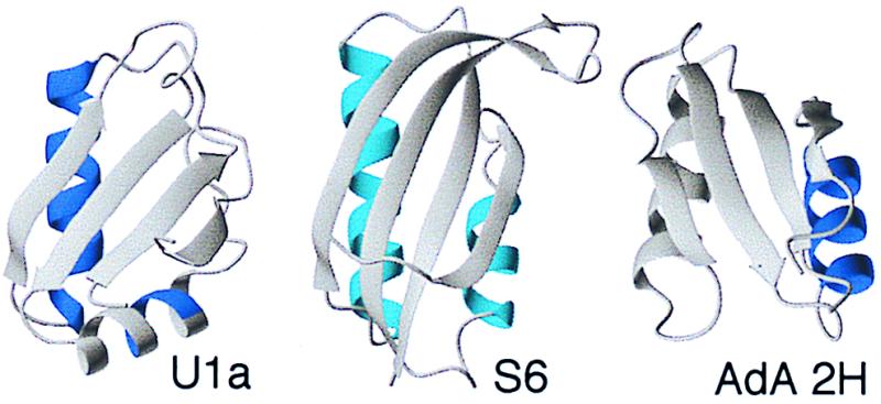
Structures of U1A, S6, and AdA 2H, indicating in blue the regions where folding starts according to φ^‡ analysis of the transition state ensemble. It appears that the split β–α–β fold contains two nucleation sites in connection with either helix. U1A nucleates mainly in helix 1 but shows also a secondary nucleation in helix 2. S6 nucleates diffusely in both sites (parallel pathways?), whereas AdA 2H nucleates in helix 2.

Abbreviation

GdmCl

guanidinium chloride

References

- 1.Fersht A R. Curr Opin Struct Biol. 1995;5:79–84. doi: 10.1016/0959-440x(95)80012-p. [DOI] [PubMed] [Google Scholar]
- 2.Gruebele M, Wolynes P G. Nat Struct Biol. 1998;5:662–665. doi: 10.1038/1354. [DOI] [PubMed] [Google Scholar]
- 3.Jackson S E. Fold Des. 1998;3:R81–R91. doi: 10.1016/S1359-0278(98)00033-9. [DOI] [PubMed] [Google Scholar]
- 4.Fersht A R. Proc Natl Acad Sci USA. 1995;92:10869–10873. doi: 10.1073/pnas.92.24.10869. [DOI] [PMC free article] [PubMed] [Google Scholar]
- 5.Shakhnovich E. Fold Des. 1998;3:R108–R111. doi: 10.1016/s1359-0278(98)00056-x. [DOI] [PubMed] [Google Scholar]
- 6.Thirumalai D, Klimov D K. Fold Des. 1998;3:112–118. doi: 10.1016/s1359-0278(98)00018-2. [DOI] [PubMed] [Google Scholar]
- 7.Matouschek A, Kellis J T, Jr, Serrano L, Fersht A R. Nature (London) 1989;342:122–126. doi: 10.1038/340122a0. [DOI] [PubMed] [Google Scholar]
- 8.Itzhaki L S, Daniel E O, Fersht A R. J Mol Biol. 1995;254:260–288. doi: 10.1006/jmbi.1995.0616. [DOI] [PubMed] [Google Scholar]
- 9.Kim P S, Baldwin R L. Annu Rev Biochem. 1990;59:631–660. doi: 10.1146/annurev.bi.59.070190.003215. [DOI] [PubMed] [Google Scholar]
- 10.Milla M E, Brown B M, Waldburger C D, Sauer R T. Biochemistry. 1995;34:13914–13919. doi: 10.1021/bi00042a024. [DOI] [PubMed] [Google Scholar]
- 11.Lopez-Hernandes I, Serrano L. Fold Des. 1996;2:43–55. [PubMed] [Google Scholar]
- 12.Burton R E, Huang G S, Daugherty M A, Calderone T L, Oas T G. Nat Struct Biol. 1997;4:305–310. doi: 10.1038/nsb0497-305. [DOI] [PubMed] [Google Scholar]
- 13.Grantcharova V P, Riddle D S, Baker D. Nat Struct Biol. 1998;5:714–720. doi: 10.1038/1412. [DOI] [PubMed] [Google Scholar]
- 14.Martinez J C, Pisabarro T M, Serrano L. Nat Struct Biol. 1998;5:721–729. doi: 10.1038/1418. [DOI] [PubMed] [Google Scholar]
- 15.Oubridge C, Ito N, Evans P R, Teo C-H, Nagai K. Nature (London) 1994;372:432–438. doi: 10.1038/372432a0. [DOI] [PubMed] [Google Scholar]
- 16.Marion D, Kay L E, Sparks S W, Torchia D A, Bax A. J Am Chem Soc. 1989;111:1515–1517. [Google Scholar]
- 17.Shaka A J, Lee C J, Pines A. J Magn Reson. 1988;77:274–293. [Google Scholar]
- 18.Cavanagh J, Rance M. J Magn Reson. 1992;96:670–678. [Google Scholar]
- 19.Bodenhausen G, Ruben D J. Chem Phys Lett. 1980;69:185–189. [Google Scholar]
- 20.Cavanagh J, Palmer A G, Wright P E, Rance M. J Magn Reson. 1991;91:429–436. [Google Scholar]
- 21.Palmer A G, Cavanagh J, Wright P E, Rance M. J Magn Reson. 1991;93:151–170. [Google Scholar]
- 22.Kay L E, Keifer P, Saarinen T. J Am Chem Soc. 1992;114:10663–10665. [Google Scholar]
- 23.Shaka A J, Barker P B, Freeman R. J Magn Reson. 1985;64:547–552. [Google Scholar]
- 24.Press W H, Flannery B P, Teukolsky S A, Vetterling W T. Numerical Recipes. The Art of Scientific Computing. Cambridge, U.K.: Cambridge Univ. Press; 1986. [Google Scholar]
- 25.Tanford C. Adv Protein Chem. 1970;24:1–95. [PubMed] [Google Scholar]
- 26.Privalov P L, Makhatadze G I. J Mol Biol. 1990;213:385–391. doi: 10.1016/S0022-2836(05)80198-6. [DOI] [PubMed] [Google Scholar]
- 27.Tan Y J, Oliveberg M, Fersht A R. J Mol Biol. 1996;264:377–389. doi: 10.1006/jmbi.1996.0647. [DOI] [PubMed] [Google Scholar]
- 28.Tanford C. Adv Protein Chem. 1968;23:121–282. doi: 10.1016/s0065-3233(08)60401-5. [DOI] [PubMed] [Google Scholar]
- 29.Oliveberg M, Fersht A R. Biochemistry. 1996;35:2726–2737. doi: 10.1021/bi9509661. [DOI] [PubMed] [Google Scholar]
- 30.Oliveberg M. Acc Chem Res. 1998;31:765–772. [Google Scholar]
- 31.Silow M, Oliveberg M. Biochemistry. 1997;36:7633–7637. doi: 10.1021/bi970210x. [DOI] [PubMed] [Google Scholar]
- 32.Matouschek A, Fersht A R. Proc Natl Acad Sci USA. 1993;90:7814–7818. doi: 10.1073/pnas.90.16.7814. [DOI] [PMC free article] [PubMed] [Google Scholar]
- 33.Oliveberg M, Tan Y-J, Silow M, Fersht A R. J Mol Biol. 1998;277:933–943. doi: 10.1006/jmbi.1997.1612. [DOI] [PubMed] [Google Scholar]
- 34.Otzen D E, Kristensen O, Procter M, Oliveberg M. Biochemistry. 1999;38:6499–6511. doi: 10.1021/bi982819j. [DOI] [PubMed] [Google Scholar]
- 35.Bryngelson J, Onuchic J N, Socci N D, Wolynes P. Proteins: Struct Funct Genet. 1995;21:167–195. doi: 10.1002/prot.340210302. [DOI] [PubMed] [Google Scholar]
- 36.Parker M J, Spencer J, Clarke A R. J Mol Biol. 1995;253:771–786. doi: 10.1006/jmbi.1995.0590. [DOI] [PubMed] [Google Scholar]
- 37.Englander W S, Sosnick T R, Mayne L C, Shtilerman M, Qi P X, Bai Y. Acc Chem Res. 1998;31:737–744. [Google Scholar]
- 38.Zaidi N F, Nath U, Udgaonkar J B. Nat Struct Biol. 1997;4:1016–1024. doi: 10.1038/nsb1297-1016. [DOI] [PubMed] [Google Scholar]
- 39.Silow M, Tan Y J, Fersht A R, Oliveberg M. Biochemistry. 1999;38:13006–13012. doi: 10.1021/bi9909997. [DOI] [PubMed] [Google Scholar]
- 40.Silow M, Oliveberg M. Proc Natl Acad Sci USA. 1997;94:6084–6086. doi: 10.1073/pnas.94.12.6084. [DOI] [PMC free article] [PubMed] [Google Scholar]
- 41.Jones C M, Henry E R, Hu Y, Chan C-K, Luck S D, Bhuyan A, Roder H, Hofrichter J, Eaton W A. Proc Natl Acad Sci USA. 1993;90:11860–11864. doi: 10.1073/pnas.90.24.11860. [DOI] [PMC free article] [PubMed] [Google Scholar]
- 42.Plotkin S S, Wang J, Wolynes P G. J Chem Phys. 1997;106:2932–2948. [Google Scholar]
- 43.Wolynes P G. Proc Natl Acad Sci USA. 1997;94:6170–6175. doi: 10.1073/pnas.94.12.6170. [DOI] [PMC free article] [PubMed] [Google Scholar]
- 44.Avis J M, Allain F H, Howe P W, Varani G, Nagai K, Neuhaus D. J Mol Biol. 1996;257:398–411. doi: 10.1006/jmbi.1996.0171. [DOI] [PubMed] [Google Scholar]
- 45.Li R, Woodward C. Protein Sci. 1999;8:1571–1590. doi: 10.1110/ps.8.8.1571. [DOI] [PMC free article] [PubMed] [Google Scholar]
- 46.Shoemaker B A, Wang J, Wolynes P G. Proc Natl Acad Sci USA. 1997;94:777–782. doi: 10.1073/pnas.94.3.777. [DOI] [PMC free article] [PubMed] [Google Scholar]
- 47.Shoemaker B A, Wang J, Wolynes P G. J Mol Biol. 1999;287:675–694. doi: 10.1006/jmbi.1999.2613. [DOI] [PubMed] [Google Scholar]
- 48.Finkelstein A V, Badredtinov A Y. Fold Des. 1997;2:115–121. doi: 10.1016/s1359-0278(97)00016-3. [DOI] [PubMed] [Google Scholar]
- 49.Lifshitz E M, Pitaevskii L P. Physical Kinetics. Oxford: Pergamon; 1981. [Google Scholar]
- 50.Villegas V, Martines J C, Aviles F X, Serrano L. J Mol Biol. 1998;283:1027–1036. doi: 10.1006/jmbi.1998.2158. [DOI] [PubMed] [Google Scholar]
- 51.Lindahl M, Svensson L A, Liljas A, Sedelnikova S E, Eliseikina I A, Fomenkova N P, Nevskaya N, Nikonov S V, Garber M B, Muranova T A, et al. EMBO J. 1994;13:1249–1254. doi: 10.2210/pdb1ris/pdb. [DOI] [PMC free article] [PubMed] [Google Scholar]