

Abstract
High-throughput technologies for genomics provide tens of thousands of genetic measurements, for instance, gene-expression measurements on microarrays, and the availability of these measurements has motivated the use of machine learning (inference) methods for classification, clustering, and gene networks. Generally, a design method will yield a model that satisfies some model constraints and fits the data in some manner. On the other hand, a scientific theory consists of two parts: (1) a mathematical model to characterize relations between variables, and (2) a set of relations between model variables and observables that are used to validate the model via predictive experiments. Although machine learning algorithms are constructed to hopefully produce valid scientific models, they do not ipso facto do so. In some cases, such as classifier estimation, there is a well-developed error theory that relates to model validity according to various statistical theorems, but in others such as clustering, there is a lack of understanding of the relationship between the learning algorithms and validation. The issue of validation is especially problematic in situations where the sample size is small in comparison with the dimensionality (number of variables), which is commonplace in genomics, because the convergence theory of learning algorithms is typically asymptotic and the algorithms often perform in counter-intuitive ways when used with samples that are small in relation to the number of variables. For translational genomics, validation is perhaps the most critical issue, because it is imperative that we understand the performance of a diagnostic or therapeutic procedure to be used in the clinic, and this performance relates directly to the validity of the model behind the procedure. This paper treats the validation issue as it appears in two classes of inference algorithms relating to genomics – classification and clustering. It formulates the problem and reviews salient results.
1. INTRODUCTION
Over the last few decades, improvements in measurement technologies have made it possible to gather ever greater detailed molecular information characterizing the state of the genome and determining the presence, absence, abundance and modification levels of the RNA and protein species being expressed in cells from normal and diseased tissue. A current international research focus is to determine how to exploit these capabilities in order to aid physicians in forming more detailed diagnoses of diseases with complex causation, thereby leading to more accurate prognosis and choice of therapeutics for treatment. The use of genomic information to develop mechanistic understandings of the relationships between genes, proteins and disease is already standard for a number of diseases. A mechanistic view that captured the straightforward way in which the relationships between genes, proteins and metabolites could be exploited in heritable diseases of metabolism was clearly formulated by Garrod in 1902 in a report of his study of alcaptonuria, a condition arising from the inability to catabolize homogentisic acid [1] and was widely disseminated through his later book, Inborn errors of metabolism [2]. Energetic collaborations between biochemists, enzymologists and geneticists used their abilities to monitor the accumulation of metabolites and the lethal effects of mutations that disable critical metabolic steps to build a very detailed understanding of the biochemistry and genomics of metabolism in bacteria and fungi. This enabled the construction of very accurate tests to diagnose the human disorders that arise when core metabolic genes are mutated. In the developed nations, a panel of such tests is typically carried out on each newborn.
This basic strategy of connecting genetic and protein information with information about the molecular pathologies underlying diseases has also been successfully employed to allow the description and diagnosis of other types of conditions arising from genomic alterations, such as Down’s Syndrome [3], and chronic myelogenous leukemia (CML) [4]. In all of these cases, an investigator finds the disease by noting that the distribution of the alteration within the population closely follows the distribution of diseased individuals within the population. Ways to test for and evaluate this kind of relationship have been extensively researched and developed in statistics. The use of this type of statistical method is common in medicine, not only in diagnostics, but also in evaluation of potential therapeutics such as drugs. Physicians are well acquainted with the basis of these analyses and have a practical knowledge of how well these analyses perform from their direct experience of the actual success and failure of therapeutics in their own hands as compared to the estimates from trials. A reasonable expectation of clinicians is that methods for diagnostic, prognostic and therapeutic utility decisions they will use in the future will be at least as well characterized for reliability as the ones currently available.
Ideally, decision-making procedures for diseases of complex causation that use classifiers based on genomic and pro-teomic features will translate into diagnostic, prognostic and therapeutic-decision tests that can be applied in a general patient population. Within this realm of application, there are two pivotal issues to consider. First, it will be necessary to develop clear understandings of how such classifiers can be formed and their accuracy established. Second, once a classifier of a given level of accuracy is developed, it will be necessary to evaluate its patterns of error on the various subsets of the patient population.
It is already apparent that even identifying the components to produce the best classifier that can be formed from a set of molecular survey observations is virtually impossible. Attempts to find fuller descriptions of the molecular pathology of complex diseases such as breast cancer, Huntington’s and Alzheimer’s are ongoing in many research institutions. In these types of disease, simple, direct mechanistic relationships between the proximate causes of the disease and the ensuing molecular pathology are not as easily established as in many metabolic diseases. In these more complex diseases, the pathology develops over long periods of time in response to the proximate causes, evolving in ways that have both general similarities and combinations of partially shared and idiosyncratic molecular features among the patients [5–8].
Another important consequence of the evolution of these diseases is that altered function is evident in a wide variety of cellular processes. In cancer it is typical to see alterations in the mechanics of proliferation signaling, survival/death signaling, error checking and metabolism. When faced with a diagnosis that only identifies a broad class of disease that may be extremely heterogeneous in its molecular pathology, the practitioner cannot accurately predict the course and severity of the disease or the best course of therapy for a particular patient. The strategy being applied to these diseases is to link genomic, proteomic and clinical observations to produce a finer grain diagnosis based on more uniform molecular pathology features that will provide practitioners with more insight into the likely course, severity and treatment vulnerability of each diagnostic type. The approach is based on identifying patterns of cellular phenotype alterations that result from the subsequent alterations in the patterns of expression and modification of RNA and protein that arise directly from genomic alterations, or indirectly from altered regulation of genomic function. This approach is based on the expectation that disease pathology requires alteration of the normal cellular phenotype and that just as in the cases of Down’s Syndrome, and CML, the resulting pathologic phenotype exhibits alterations in its constituent RNA and protein components [9, 10].
The availability of various microarray technologies that allow simultaneous measurements of the abundance of many mRNA species present in a tissue has enabled considerable exploratory work to establish that patterns of mRNA abundance appear to be linked to various aspects of cancer phenotypes. These include the tissue of origin of the tumor [11, 12], pathological subclasses of tumors [13, 14], traditional clinical features [15], treatment susceptibility [16], and prognosis [7, 14, 17]. While it seems likely that ways can be developed to convert these apparent associations to quantitatively characterized tests, a considerable complexity problem is associated with this translation. The situation is exacerbated by sample sets that likely contain substantially differing types of molecular pathologies, each of which will probably require multiple features to recognize. Much initial work in the area has relied on non-predictive methods designed for identifying gross trends in the data, such as clustering, principal component analysis, multidimensional scaling, and the like. There have also been efforts to use predictive methods, such as classification; however, these have been carried out under conditions, such as very small samples, not conducive to many existing methods [18]. Examples of the issues facing gene-based classification are complex classifier design [19], error estimation [20, 21], and feature selection [22–24].
Taking a general scientific perspective, if we loosely define genomics as the study of large sets of genes with the goal of understanding collective gene function, as opposed to just that of individual genes, then in comparison to classical genetics, gene biology has moved into an entirely new realm, one fraught with theoretical and experimental difficulties. The scale of system integration confronting us is far greater than any human-built system, and thus we have little intuitive understanding of how it is accomplished. Not only is the dimensionality greater by orders of magnitude than that experienced by human beings in their everyday, common sense experience, but the system exhibits control that is multivariate, nonlinear, and distributed. Add to this the inherent model stochasticity, and one is inexorably confronted in ge-nomics by a science whose basic tenets must be approached in the context of high-dimensional stochastic nonlinear dynamical systems. Based upon experience, nothing could be more daunting.
In the past one might have accepted a biological epistemology in which a proposed system could be evaluated by reasoning about it in relation to gathered data. That is, the validity of a proposed model could be asserted based on is reasonableness. Such an epistemology cannot be entertained when one is dealing with high-dimensional stochastic dynamical systems because one cannot expect the behavior of such a system to behave “reasonably.” The number of variables, their multivariate interaction, and the probabilistic nature of the resulting state space make it impossible for human intuition to assert the degree to which system behavior is consistent with the physical behavior of the observables to which its variables correspond. Quoting Dougherty and Brag-Neto [25], “Human intuition and vocabulary have not developed with reference to any experience at the subatomic level or the speed of light, nor have they developed with reference to the kinds of massive nonlinear systems encountered in biology. The very recent ability to observe and measure complex, out of the ordinary phenomena necessitates scientific characterizations that go beyond what seems ‘reasonable’ to ordinary understanding.” This is not to say that model construction does not require keen insight and creativity, only that inter-subjective model validation will require a formal validation procedure. Even for such a simple gene regulatory network model as the Boolean model [26, 27], slight changes in the model parameters can result in startlingly different long-run behavior, and it would be fruitless for scientists to debate the efficacy of the model in a particular application without verifying that it produces steady-state behavior that is predictive of that experimentally observed. The validity of a scientific model rests on its ability to predict behavior. The criteria of validity must be rigorously formulated. These may vary depending on ones goals. In this sense validity possesses a pragmatic aspect. For instance, it may be that we desire a network model whose steady-state behavior models steady-state behavior of a cell. Should this be the case, our characterization of validity will be less stringent than if we insist that model predictions agree for both transient and steady-state measurements. Moreover, owing to the inherent stochastic nature of the modeling, validity criteria must be set in a probabilistic framework.
Owing to the complexity and sheer magnitude of the variables and relations within genomics, it is evident that the representation of the relations will require complex mathematical systems, such as differential-equation and graphical models, which ultimately means that computational biology (or systems biology) will provide the theoretical ground. But this in turn means that the science of genomics will find its expression within a contemporary epistemology of computational biology, one that is based on predictive models, not a posteriori explanations [25]. The relations between variables that constitute the scientific knowledge will be described within a mathematical model. Just as importantly, the connection between the model and the biological universe will be manifested via measurable consequences of the theory; that is, the abstract mathematical structure constituting the theory must be checked for its concordance with sensory observations. This is accomplished by making predictions from the theory that correspond to experimental outcomes. To constitute scientific knowledge, the model must be validated.
Currently in genomics, validation is problematic. Mehta, Murat, and Allison write [28], “Many papers aimed at the high-dimensional biology community describe the development or application of statistical techniques. The validity of many of these is questionable, and a shared understanding about the epistemological foundations of the statistical methods themselves seems to be lacking.” In this paper we review the state of validation for two computational paradigms currently being extensively employed in genomics: classification and clustering. Two points will become clear: first, insufficient attention has been paid to validation; and second, where suitable validation methodologies exist, too little attention is being paid to them in genomic science. Clustering provides an instance of the first point, where for the most part clustering has been applied without concern for predictive validation, and where so-called “validation indices” have been applied without attention being paid as to whether these “validation indices” provide any validation in the scientific sense. Classification provides an instance of the second point, where validation inheres in the process of error estimation and estimation procedures have been applied without regard for their precision, imprecision being a manifestation of invalidity.
2. CLASSIFICATION
Expression-based classification involves a classifier that takes a vector of gene expression levels as input and outputs a class label, or decision. For a typical example, we consider patient data from a microarray-based classification study that analyzes microarrays prepared with RNA from breast tumor samples from 295 patients [29]. Of the 295 microarrays, 115 belong to the “good-prognosis” class and 180 belong to the “poor-prognosis” class. From the original published data set, the expression profiles of 70 genes were found to be the most correlated with disease outcome [30]. From among these 70, two genes, LOC51203 and Contig38288_RC (AN), have been found to be the most discriminating for linear classification, the result of classifier design via linear discriminant analysis (LDA) being shown in Fig. (1), with reported estimated error 0.0582 [31]. In this case, given such a simple classifier, the sample used to design the classifier and estimate the error is fairly large and one might feel confident that the designed classifier will work with approximately the same performance on the population as it does on the sample; namely, its error on the population will agree with the error estimate obtained from the sample; however, much smaller sample sizes are commonplace in the literature. For instance, Fig. (2) shows a linear gene-expression classifier for separating CD5+ and CD5− diffuse large B-cell lympho-mas (DLBCLs) using two genes, integran β1 and CD36, where the sample consists of 11 and 9 patients for CD5+ and CD5−, respectively, with reported estimated error 0.141 [32].
Fig. (1).

Linear classifier separating patients with good and bad prognosis using two genes.
Fig. (2).

Linear classifier separating CD5+ and CD5− DLBCLs.
Given the small sample, making claims about classifier performance (error) on the population is problematic. We are confronted by the issue of classifier model validity, which relates directly to the quality of error estimation [25].
Before addressing the question formally, let us step back and consider what lies behind a classifier such as the ones depicted in Figs. (1 and 2). To do so, let us leave the particular studies and consider expression-based classification from a generic perspective. Suppose we wish to discriminate be-tween phenotypes A0 and A1, and we have strong biological evidence to believe that the different phenotypes result from production of a single protein P controlled by transcription factors, X1 and X2. Specifically, when X1 and X2 bind to the regulatory region for gene G, the gene expresses, the corresponding mRNA is produced, and this translates into the production of protein P, thereby resulting in phenotype A1; on the other hand, in the absence of either X1 or X2 binding, there is no transcription and phenotype A0 is manifested. A simple quantitative interpretation of this situation is that there exist expression levels κ1 and κ2 such that phenotype A1 is manifested if X1 > κ1 and X2 > κ2, whereas A0 is mani-fested if either or . These conditions charac-terize the desired classifier, defined by if X1 >κ1 and , and if or , where phenotype is treated as a binary target variable Y with Y = 0 corresponding to A0 and Y = 1 corresponding to A1. If these conditions were to strictly hold, then the classifier would have error ; however, owing to concentration fluctuations, time delays, and the effects of other variables, one cannot expect to have a perfect classifier. Hence, the actual error would be of the probabilistic form
| 1 |
Were the joint distribution for the transcription factors and phenotype known, this error could then be directly computed. The result would be a classifier model consisting of the classifier ψ and its error
From a practical perspective, the preceding scenario is highly idealized. Let us examine what happens when we back off the idealization. First, assume that we do not know the joint distribution of the transcription factors and phenotype. In this case the error has to be estimated. This could be done by taking a data sample consisting of points of the form ((X1, X2), Y), transcription vector and phenotype, applying the classifier to each transcription pair (X1, X2) to arrive at a predicted phenotype , and taking the error estimate as the proportion of incorrect predictions. The proportionality estimation procedure is called an error estimation rule. Whereas in the first scenario the full model, classifier and error, are derived from theoretical considerations, in the second, the classifier is derived from theoretical considerations but the error is estimated from data. If the data set is very large, then we can expect the error estimate to be very close to the true error, meaning that the expected deviation is small; however, if the data set is small, we cannot expect to be small. Thus, in a sense that must be rigorously defined, the validity of the model relates to the quantity of data used to arrive at the estimate, as well as the difficulty of making the estimate.
Suppose that we do not know the thresholds and , only that phenotype A1 occurs if and only if the transcription factors are both sufficiently expressed. Then we could proceed by developing a procedure, called a classification rule, that upon being applied to sample data, called training data, yields estimates, and , of and , respectively. This would provide us with a classifier, , that is an estimate of the desired classifier, ψ. Going further, we might not have any biological knowledge that gives us confidence that the classifier should be of the form , if and only if X1 > κ1 and X2 > X2 > κ2. In this typical scenario, we need to use a classification rule that assumes some “reasonable” form for the classifier, such as a linear classifier, and then estimates the particulars of the classifier from training data. In either case, to obtain an estimate, of the error, , of ψest, we could either take additional sample data, called test data, to form the estimate via some error estimation rule, or we could simply apply some error estimation rule to the training data. Given no limitations on cost or data availability, we would like to have large samples for both classifier design and error estimation; however, in practice, this is often impossible. In expression-based classification, data are usually severely limited, so that holding out test data results in unacceptably poor classifier design. Thus, design and error estimation must be done on the same training data. This has consequences for validity because validity relates to the accuracy of the error estimate.
3. VALIDITY OF CLASSIFIER MODELS
Having motivated the discussion of validity with a generic transcription example, we now turn to a formal analysis of the issues. We begin by providing a brief description of the probabilistic theory of classification [33]. Classification involves a feature vector on d-dimensional Euclidean space composed of random variables (features), a binary random variable Y, and a function (classifier) for which is to predict Y. The values, 0 or 1, of Y are treated as class labels. Given a feature-label distribution fX,Y(x, y), the error, , of ψ is the probability of erroneous classification, namely, . The error is relative to a feature-label distribution . It equals the expected (mean) absolute difference, , between the label and the classification. Owing to the binary nature of and Y, it also equals the mean-square error. A classifier ψ is optimal (best) for a feature-label distribution for any classifier . An optimal classifier, , of which there may be more than one, and its error, , are deducible via integration from the feature-label distribution. These are called a Bayes classifier and the Bayes error, respectively.
To address validity in the context of classification, we need an appropriate definition of the model. We define a classifier model to be a pair composed of a function and a real number and are called the classifier and error, respectively, of the model M. The mathematical form of the model is abstract, with not specifying an actual error probability corresponding to ψ. M becomes a scientific model when it is applied to a feature-label distribution. The model is valid for the distribution fX,Y to the extent that approximates . Hence, quantification of model validity is relative to the absolute difference .
In practical applications, the feature-label distribution is usually unknown, so that a classifier and its error are generally discovered via classification and error estimation rules. Given a random sample of pairs drawn from a feature-label distribution , we desire a function on Sn that yields a good classifier. The randomness of Sn means that any particular sample Sn is a realization of Sn . A classification rule is a mapping of the form , where Fd is the family of -valued functions on Rd. Given a specific sample Sn of Sn, we obtain a designed classifier according to the rule ψ. The classifier is then of the form . To simplify notation, we write instead of , keeping in mind that the classifier has been designed from a sample. Note that a classification rule is really a sequence of classification rules depending on n. The error term in the model is estimated by an estimation rule, . Although there is no logical necessity, we will assume that the classifier is part of the estimation rule (else one would be estimating the error independent of the classifier). Altogether, we arrive at a scientific model via a creative act that postulates a rule model and then via computation from a data sample arrives at the scientific model.
We must consider the validity of a classifier model M = under the assumption that both and ψ have been arrived at via the rule model . Thus, we consider the model , where and for sample data set Sn. Model validity relates to the precision of Ξ as an estimator of : if an estimation rule is expected to yield an error close to the true error of the designed classifier, then we have confidence in the validity of the model. Relative to validity, we are concerned with the precision of the error estimator in the model , which can be considered random, depending on the sample.
The precision of the estimator relates to the difference between and , and we require a probabilistic measure of this difference. Here we use the root-mean-square error (square root of the expectation of the squared difference),
| 2 |
Error-estimation precision depends on the classification rule Ψ, error estimation rule Ξ, feature-label distribution f, and sample size n.
It is helpful to understand the RMS in terms of the devia- tion distribution, . The RMS can be decom-posed into the bias, of the error estimator relative to the true error, and the deviation variance, , namely,
| 3 |
where we recognize that Ψ, Ξ, f, and n are implicit on the right-hand side.
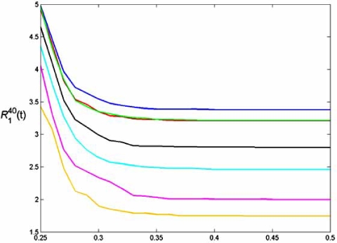
There are rare instances in which, given the feature-label distribution, the exact analytic formulation of the RMS is known. Here we consider multinomial discrimination, where the feature components are random variables with discrete range , corresponding to choosing a fixed-partition in with b cells, and the histogram rule assigns to each cell the majority label in the cell. Exact analytic formulations of the RMS for resubstitution and leave-one-out error estimation are known [34]. The expressions are complicated and we omit them. As we expect, they show that the RMS decreases for decreasing b. They also show that for a wide range of distributions, resubstitution outperforms leave-one-out for 4 and 8 cells. Rather than just give some anecdotal examples for different distributions, we consider a parametric Zipf model, which is a power-law discrete distribution where the parameter controls the difficulty of classification. Fig. (3)shows the RMS as a function of the expected true error computed for a number of distinct models of the parametric Zipf model for n = 40 and b = 8. Their performances are virtually the same (resubstitution slightly better) for , which practically means equivalent performance in any situation where there is acceptable discrimination. for b = 4 (not shown), resubstitution outperforms leave-one-out across the entire error range and for b = 16 (not shown) re-substitution is very low-biased and leave-one-out has better performance. For the Boolean model for gene regulation, b = 2, 4, 8, and 16 correspond to network connectivity 1, 2, 3, and 4, respectively, connectivity being the number of genes that predict the state of any other gene in the network. Since in practice connectivity is often bounded by 3 and there is need to estimate the errors of tens of thousands of predictor functions, there is a big computational benefit in using re-substitution, in addition to better prediction for 1 and 2 predictors.
Fig. (3).

RMS as a function of the expected true error computed for a number of distinct models of the parametric Zipf model for n = 40 and b = 8. Cross marker: resubstitution; circle marker: leave-one-out.
4. GOODNESS OF CLASSIFIER MODELS
A model may be valid relative to the RMS of the error estimator being small; however, is it any good? The quality of goodness does not apply to the model M, but only to the classifier. Classifier ψ is better than classifier φ relative to the distribution f if . Obviously, a Bayes classifier is best among all possible classifiers. We need to consider goodness of classifier ψ in the model under the assumption that both ψ and have been arrived at via the rule model . Note that it is just as well to com-pare , as compare to , both of which exceed the Bayes error . Hence, the relative goodness of a designed classifier can be measured by its design cost . From the perspective of the classification rule, and are sample-dependent random variables. Thus the salient quantity for a classification rule is the expected design cost, , the expectation being relative to the random sample Sn. The expected error of the designed classifier is decomposed as
| 4 |
Qualitatively, a rule is good if is small.
A well-known difficulty with small-sample design is that E tends to be unacceptably large. A classification rule may yield a classifier that performs well on the sample data; however, if the small sample does not generally represent the distribution sufficiently well, then the designed classifier will not perform well on the distribution. This phenomenon is known as overfitting the sample data. Relative to the sample the classifier possesses small error; but relative to the feature-label distribution the error may be large. The overfitting problem is not necessarily overcome by applying an error-estimation rule to the designed classifier to see if it “actually” performs well, since error-estimation rules are very imprecise in small-sample settings. Even with a low error estimate, is one sufficiently confident in the accuracy of that estimate to overcome the large expected design error owing to using a complex classifier with a small data set? We need to consider classification rules that are constrained so as to reduce overfitting.
Constraining classifier design means restricting the functions from which a classifier can be chosen to a class C. Constraint can reduce the expected design error, but at the cost of increasing the error of the best possible classifier. Since optimization in C is over a subclass of classifiers, the error of an optimal classifier, , in C will typically exceed the Bayes error, unless . This cost of constraint is . A classification rule yields a classifier with error , and . Design error for constrained classification is . For small samples, this can be much less than Δf,n, depending on C and the rule. The expected error of the designed classifier from C can be decomposed as
| 5 |
The constraint is beneficial if and only if , which is true if the cost of constraint is less than the decrease in expected design cost. The dilemma is that strong constraint reduces at the cost of increasing .
Generally speaking, the more complex a class C of classifiers, the smaller the constraint cost and the greater the design cost. By this we mean, the more finely the functions in C partition the feature space , the better functions within it can approximate the Bayes classifier and, concomitantly, the more they can overfit the data. As it stands, this statement is too vague to have a precise meaning. Since our interest in this paper is validity (therefore, error estimation), let us simply note a celebrated theorem that provides bounds for . It concerns the empirical-error classification rule, which chooses the classifier in C that makes the least number of errors on the sample data. For this (intuitive) rule, satisfies the bound
| 6 |
where VC is the VC (Vapnik-Chervonkis) dimension of C [19]. We will not go into the details of the VC dimension, except to say that it provides a measure of classifier complexity. It is clear from Eq. 6 that n must greatly exceed VC for the bound to be small. The VC dimension of a linear classifier is d + 1. For a neural network with an even number k of neurons, the VC dimension has the lower bound . If k is odd, then . Thus, for a even number of neurons, we deduce from Eq. 6 that the bound exceeds , which is not promising for small n.
5. BEHAVIOR OF TRAINING-DATA ERROR ESTIMATORS
In this section we will consider the deviation distributions of some well-known training-data-based error estimators and compare their biases and variances.
Upon designing a classifier ψn from the sample, the re-substitution estimate, , is given by the fraction of errors n made by on the sample. The resubstitution estimator is typically low-biased, meaning , and this bias can be severe for small samples, depending on the complexity of the classification rule.
Cross-validation is a re-sampling strategy in which (surrogate) classifiers are designed from parts of the sample, each is tested on the remaining data, and classifier error is estimated by averaging the errors. In k-fold cross-validation, the sample Sn is partitioned into k folds S(i), for i = 1, 2,…, k. Each fold is left out of the design process and used as a test set, and the estimate, , is the average error committed n on all folds. A k-fold cross-validation estimator is unbiased as an estimator of , meaning , where is the error arising from de-sign on a sample of size n − n/k. The special case of n-fold cross-validation yields the leave-one-out estimator, which is an unbiased estimator of . While not suf fering from severe bias, cross-validation has large variance in small-sample settings, the result being high RMS [20]. In an effort to reduce the variance, k-fold cross-validation can be repeated using different folds, the final estimate being an average of the estimates.
Bootstrap is a general re-sampling strategy that can be applied to error estimation [35]. A bootstrap sample consists of n equally-likely draws with replacement from the original sample Sn. Some points may appear multiple times, whereas others may not appear at all. For the basic bootstrap estimator, , the classifier is designed on the bootstrap sample and tested on the points left out, this is done repeatedly, and the bootstrap estimate is the average error made on the left-out points. tends to be a high-biased estimator of since the number of points available for design is on average only 0.632n. The .632 bootstrap estimator tries to correct this bias via a weighted average of and resubstitution [36],
| 7 |
Looking at Eq. 7, we see that the .632 bootstrap is a convex combination of a low-biased and high-biased estimator. As such it is a special case of a convex estimator, the general form of which is
| 8 |
[37]. Given a feature-label distribution, a classification rule, and low and high-biased estimators, an optimal convex estimator is found by finding the weights a and b that minimize the RMS.
In resubstitution there is no distinction between points near and far from the decision boundary; the bolstered-resubstitution estimator is based on the heuristic that, relative to making an error, more confidence should be attributed to points far from the decision boundary than points near it [38]. This is achieved by placing a distribution, called a bolstering kernel, at each point and estimating the error by integrating the bolstering kernels for all misclassified points (rather than simply counting the points as with resubstitu-tion). A key issue is the amount of bolstering (spread of the bolstering kernels), and a method has been proposed to compute this spread based on the data. Fig. (4) illustrates the error for linear classification when the bolstering kernels are uniform circular distributions. When resubstitution is heavily low-biased, it may not be good to spread incorrectly classified data points because that increases the optimism of the error estimate (low bias). The semi-bolstered-resubstitution estimator results from not bolstering (no spread) for incorrectly classified points. Bolstering can be applied to any error-counting estimation procedure. Bolstered leave-one-out estimation involves bolstering the resubstitution estimates on the surrogate classifiers.
Fig. (4).

Bolstered resubstitution for linear classification.
To demonstrate small-sample error-estimator performance for continuous models, we provide simulation results for the distribution of the deviation , in which the error estimator is one of the following: resubstitution (resub), leave-one-out (loo), 10-fold cross-validation with 10 repetitions (cv10r), .632 bootstrap (b632), bolstered resubsti-tution (bresub), semi-bolstered resubstitution (sresub), or bolstered leave-one-out (bloo). Bolstering utilizes Gaussian bolstering kernels. Based upon the patient data corresponding to Fig. (1), the simulations use log-ratio gene-expression values associated with the top 5 genes, as ranked by a correlation-based measure. For each case, 1000 observations of size n = 20 and n = 40 are drawn independently from the pool of 295 microarrays. Sampling is stratified, with half of the sample points being drawn from each of the two prognosis classes. The true error for each observation of size n is approximated by a holdout estimator, whereby the 295 − n sample points not drawn are used as the test set (a good approximation to the true error, given the large test sample). This allows computation of the empirical deviation distribution for each error estimator using the considered classification rules. Since the observations are not independent, there is a degree of inaccuracy in the computation of the deviation distribution; however, for sample sizes n = 20 and n = 40 out of a pool of 295 sample points, the amount of overlap between samples is small (see [20] for a discussion of this sampling issue). Fig. (5) displays plots of the empirical deviation distributions for LDA obtained by fitting beta densities to the raw data. A centered distribution indicates low bias and a narrow distribution indicates low variance. Note the low bias of resubstitution and the high variance of the cross-validation estimators. These are generally outperformed by the bootstrap and bolstered estimators; however, specific performance advantages depend heavily on the classification rule and feature-label distribution.
Fig. (5).

Beta-distribution fits for the deviation distributions of several estimation rules. Left: n = 20; right: n = 40.
6. CONFIDENCE BOUNDS ON THE ERROR
A natural question to ask is what can be said of the true error, given the estimate in hand. This question pertains to the conditional expectation of the true error given the error estimate. In addition, one might be interested in confidence bounds for the true error given the estimate. These issues are addressed via the joint distribution of the true error and the estimated error, from which can be derived the marginal distributions, the conditional expectation of the estimated error given the true error, the conditional expectation of the true error given the estimated error, the conditional variance of the true error given the estimated error, and the 95% upper confidence bound for the true error given the estimated error [39]. The joint distribution concerns the random vector of the true and estimated errors, and , respectively. To obtain results reflecting what occurs in practice, where one does not know the feature-label distribution, we assume that the feature-label distribution is random, so that depends on both the random choice of feature-label distribution and random sample from that distribution.
Of key concern is the conditional expectation, , of the true error given the estimated error, because in practice one has only the estimated error and, given this, , is the best mean-square-error estimate of the true error. An estimator might be low-biased from a global perspective, meaning it is low-biased relative to its marginal distribution, but it may be conditionally high-biased for certain values of the estimated error.
A second major concern is finding a conditional bound for the true error given the joint error distribution. In many settings, one is not primarily interested in the error of a classifier but is instead concerned with the error being less than some tolerance. For instance, in developing a prognosis test for survivability, one is not likely to be concerned as much with the exact error rate but rather that the error rate is beneath some acceptable bound. In this situation, typically low-biased error estimators such as resubstitution are considered especially unacceptable. Less-biased, high-variance error estimators like cross-validation are also problematic because they will often significantly underestimate the true error. But here one must be cautious. If tolerance is the issue, rather than simply look at bias or variance, a more precise way to evaluate an error estimator is to consider a bound conditioned on the error estimate: given the error estimate , we would like a conditional bound on of the form
| 9 |
The subscript n on the bound indicates that it is a function of the random sample. In this setting, a classification rule ψ is better than the rule Ω for . ψ is uniformly better than Ω over the interval for all .
To illustrate the construction of conditional bounds (and some other issues in the sequel), we will consider two equally likely Gaussian class-conditional distributions with covariance matrices, K0 and K1. For the linear model, K1 = K0 and the Bayes classifier results from linear discriminant analysis (LDA); for the quadratic model, K1 = 2K0 and the Bayes classifier results from quadratic discriminant analysis (QDA). The particular model for any application depends on the choice of K0. The application depends on the classification rule applied.
Here we consider the LDA classification rule applied to the quadratic model with
| 10 |
where is Q is a 5 75 matrix with 1 on the diagonal and ρ = 0.25 off the diagonal. The classes are separated so that the expected Bayes error is 0.15. Because covariance matrices are different, the optimal classifier is quadratic. We consider several error estimators: leave-one-out cross-validation (loo), resubstitution (resub), 5-fold cross-validation with 20 replications (cv), 0.632 bootstrap (b632), bolstered resubstitution (bresub), and semi-bolstered resubstitution (sresub). The joint distributions have been estimated by massive simulation on a Beowulf cluster.
Curves for the conditional expectation of the true error given the estimated error are shown in Fig. (6a), where the dotted 45-degree line corresponds to the conditional expected estimated error equaling the true error, the estimated-error means are marked on the horizontal axis, and the true-error mean is marked on the vertical axis. The key point is that the conditional expected true error varies widely around the estimated error across the range of the estimated error. The conditional expected true error is larger than the estimated error for small estimated errors and is often smaller than the estimated error for large estimated errors. The curves of the high-variance cross-validation estimators begin well above the 45 degree and end well below it.
Fig. (6).


Conditional curves: (a) Conditional expectation of the true errors given the estimated errors; (b) Conditional 0.95 bounds for the true errors given the estimated errors.
A second concern is the formation of conditional bounds for the true error. Curves for the conditional 0.95 bounds are shown in Fig. (6b) for the model being considered. As in the case of the conditional expected true error, the means of the estimated errors are marked on the horizontal axis in the figure, but here, besides the star marking the mean true error on the vertical axis, there are also marks giving the mean 0.95 conditinal bounds across all estimated errors. Given an estimated error, a lower bound is better. For most of the estimated error range, and well beyond the mean of the true error, the semi-bolstered resubstitution bound is the best. What is perhaps most surprising, and not uncommon for other models and classification rules, is the closeness of the mean bounds on the vertical axis. While on average the conditional bounds for bolstered and semi-bolstered resubstitution are slightly lower than the others, there is not much difference, including the mean for the resubstitution bound. At first this might seem remarkable since the conditional-bound curve for resubstitution is so much above the other curves. But we must remember that the mean for the resubstitution estimate is much lower, so that the mass of the resubstitution estimate is concentrated towards the left of the conditional-bound curve, whereas the masses of the other estimates are concentrated much more towards the right of their conditional-bound curves.
7. BOUNDS FOR THE DEVIATION BETWEEN ESTIMATED AND TRUE ERRORS
Since the feature-label distribution can strongly affect the RMS and is unknown in practice, a distribution-free upper bound of the form can be useful, even if the inequality is likely to be loose.
For the resubstitution and leave-one-out estimators in the context of multinomial discrimination and the histogram rule, there exist classical upper bounds on the RMS:
| 11 |
| 12 |
where denote the histogram rule for b cells, resubstitution estimation rule, and leave-one-out estimation rule, respectively [33]. For n = 100, , indicating the bound is not useful for small samples. The bounds contain asymptotic information. For instance, faster than faster than as , indicating that resubstitution is better than leave-one-out for large samples. For small samples, the resubstitution bound may still be less than the leave-one-out bound when the number of cells is small.
The k-nearest-neighbor rule assigns to a point the majority label among its nearest k neighbors in the sample, and an upper bound on RMS is available for leave-one-out:
| 13 |
[40]. For the popular choice k = 3, at n = 100, .
The kernel rule computes the weight of each sample point on the target sample point based on a kernel function, and assigns the label of largest overall weight. For a regular kernel of bounded support and the leave-one-out estimator, the RMS is bounded by:
| 14 |
where C1 and C2 are constants depending only on d and the kernel function, respectively [33].
8. RANKING FEATURE SETS
An important application is to rank gene sets based on their ability to classify phenotypes. Since there may be many gene sets that can provide good discrimination, one may wish to find sets composed of genes for which there is evidence of their molecular relationship with the phenotype of interest. The idea is that good feature sets may provide good candidates for diagnosis and therapy. Given a family of gene sets discovered by some classification rule, the issue is to rank them based on error. Thus, a natural measure of worth for an error estimator is its ranking accuracy for feature sets [41, 42]. The measure will depend on the classification rule and the feature-label distribution. We use two measures of merit. Each compares ranking based on true and estimated errors – under the condition that the true error is less that t. is the number of feature sets in the truly top K feature sets that are also among the top K feature sets based on error estimation. It measures how well the error estimator finds top feature sets. is the mean-absolute rank deviation for the K best feature sets.
Again we consider the patient data associated with Fig. (1) and LDA classification. We consider all feature sets of size 3. For each sample of size 30 we obtain the LDA classifier and obtain the true error from the distribution and estimated errors based on resubstitution, cross-validation, bootstrap, and bolstering. We use log-ratio gene expression values associated with the top 20 genes ranked according to [30]. The true error for each sample of size of 30 is approximated by a hold-out estimator, whereby the 265 sample points not drawn are used as the test set (a very good approximation to the true error, given the large test sample). Fig. (8) shows graphs obtained by averaging these measures over many samples [41]. Cross-validation is generally poorer than the .632 bootstrap, whereas the bolstered estimators are generally better.
Fig. (8).
Feature-ranking measures for breast-cancer data: (a) RK(t) ; (b) RK (t)
9. FEATURE SELECTION
In addition to complexity owing to the structure of the classification rule; complexity also results from the number of variables. This can be seen in the VC dimension, for instance, of a linear classification rule whose VC dimension is d + 1, where d is the number of variables. This dimensionality problem motivates feature (variable) selection when designing classifiers. When used, a feature-selection algorithm is part of the classification rule, and, relative to this rule the number of variables is the number in the data measurements, not the final number used in the designed classifier. Feature selection results in a subfamily of the original family of classifiers, and thereby constitutes a form of constraint. Feature selection yields classifier constraint, not a reduction in the dimensionality of the feature space relative to design. Since its role is constraint, assessing the worth of feature selection involves us the standard dilemma: increasing constraint (greater feature selection) reduces design error at the cost of optimality. And we must not forget that the benefit of feature selection depends on the feature-selection method and how it interacts with the rest of the classification rule.
9.1. Peaking Phenomenon
A key issue for feature selection concerns error monotonicity. The Bayes error is monotone: if A and B are feature sets for which A ⊂ B, then , where εA and εB are the Bayes errors corresponding to A and B, respectively.
However, if εA,n and εB,n are the corresponding errors resulting from designed classifiers on a sample of size n, then it cannot be asserted that εA,n ≥ εB,n. It may even be that E[εB,n] > E[>A,n]. Indeed, it is typical for the expected design error to decrease and then increase for increasingly large feature sets.
Thus, monotonicity does not apply to designed classifiers. Moreover, even if εA,n ≥ εB,n, this relation may be reversed when using estimates of the errors.
To more closely examine the lack of monotonicity for designed classifiers, consider a sequence, x1, x2,…, xd,…, of features, and a sequence, Ψ1, Ψ2,…, Ψd,…, of classification rules, for which Ψd yields a classifier possessing dependent variables x1, x2,…, xd, and the rule structure is independent of d – for instance, Ψd is defined by quadratic discriminant analysis of dimension d or by the 3-nearest-neighbor rule of dimension d. What commonly (but not always) happens is that the greater complexity of the classification rule improves classifier design up to a point, after which overfitting results in sufficiently increasing design error that design deteriorates. This decrease and then rise in error as the number of features increases is called the peaking phenomenon [43, 44]. The optimal number of features depends on the classification rule, feature-label distribution and sample size [45, 46]. Typically (but not always), the optimal number of features increases with the sample size.
To illustrate the commonplace understanding of the peaking phenomenon and a couple of anomalies we employ both the linear and quadratic models, with the covariance matrix
| 15 |
of dimension 30. Features within the same block are correlated with correlation coefficient ρ and features in different blocks are uncorrelated. There are m groups, with m being a divisor of 30. We denote a particular feature by xij, where i, 1 ≤ i ≤ m, denotes the group to which the feature belongs and j, 1 ≤ j ≤ r, denotes its position in the group. We list the feature sets in the order x11, x21,…, xm1, x12,…, xmr. Since the maximum dimension considered is 30, the peaking phenomenon will only show up in the graphs for which peaking occurs with less than 30 features.
Fig. (9a) exhibits the typical understanding of peaking. It is for the LDA classification rule applied to the linear model with m = 5 groups, ρ = 0.125, and the variance σ2 set to give a Bayes error of 0.05. For fixed sample size, the curve is concave, the optimal number of features is given by the unique minimum of the curve, and the optimal number increases as the sample size increases. Note that the sample size must exceed the number of features to avoid degeneracy. The situation is quite different in part (b) of the figure. Here, a linear support vector machine (SVM) is applied to the nonlinear model with m = 1 group, ρ = 0.25, and the variance σ2 set to give a Bayes error of 0.05. First, the curves are not necessarily convex; and second, the optimal number of features does not decrease with an increasing sample size (and here are not referring to the slight wobble in the curve owing to error estimation).
Fig. (9).
Optimal number of features: (a) LDA, linear model; (b) linear SVM, nonlinear model.
9.2. Feature-Selection Algorithms
In the preceding examples, we knew the distributions and ordered the features so as not to have to consider all possible feature sets; in practice, the features are not ordered and a good feature set must be found from among all possible feature subsets. Here we are confronted by a fundamental limiting principle: to select a subset of k features from a set of d features and be assured that it provides an optimal classifier with minimum error among all optimal classifiers for subsets of size k, all k-element subsets must be checked unless there is distributional knowledge that mitigates the search requirement [47]. The intractability of a full search leads to the necessity of suboptimal feature selection algorithms.
Many feature selection algorithms have been proposed in the literature. Here we consider only three. A simple method is simply to examine one feature at time via the t-test to determine which features best separate the classes in a single dimension relative to separation of the means normalized by the variance in a given dimension. This method suffers from two drawbacks: (1) it may reject features that are poor in and of themselves but work well in combination with other features; and (2) in can yield a list of redundant features. A common approach to overcome these drawbacks is sequential selection, either forward or backward, and their variants. Sequential forward selection (SFS) begins with a small set of features, perhaps one, and iteratively builds the feature set. When there are k features, x1, x2,…, xk, in the growing feature set, all feature sets of the form {x1, x2,…, xk, w} are compared and the best one chosen to form the feature set of size k + 1. A problem with SFS is that there is no way to delete a feature adjoined early in the iteration that may not perform as well in combination as other features. The SFS look-back algorithm aims to mitigate this problem by allowing deletion. For it, when there are k features, x1, x2,…, xk, in the growing feature set, all feature sets of the form {x1, x2,…, xk, w, z} are compared and the best one chosen. Then all (k + 1)-element subsets are checked to allow the possibility of one of the earlier chosen features to be deleted, the result being the k + 1 features that will form the basis for the next stage of the algorithm. Flexibility can be added by considering sequential forward floating selection (SFFS), where the number of features to be adjoined and deleted is not fixed [48]. For a large number of potential features, feature selection is problematic and the best method depends on the circumstances. Evaluation of methods is generally comparative and based on simulations, and it has been shown that SFFS can perform well [49, 50]; however, as we will now demonstrate, SFFS can be severely handicapped in small-sample settings by poor error estimation.
9.3. Impact of Error Estimation on Feature-Selection Algorithms
When selecting features via an algorithm like SFFS that employs error estimation within it, the choice of error estimator significantly impacts feature selection, the degree depending on the classification rule and feature-label distribution [22]. To illustrate the issue, we consider two 20-dimensional unit-variance spherical Gaussian class conditional distributions with means at δa and −δa, where a = (a1, a2,…, a20), |a| = 1, and δ > 0 is a separation parameter. The Bayes classifier is a hyperplane perpendicular to the axis joining the means. The best feature set of size k corresponds to the k largest parameters among {a1, a2,…, a20}. We consider SFS and SFFS feature selection, and the LDA and 3NN rules, and select 4 features from samples of size 30. Table 1 gives the average true errors of the feature sets found by SFS, SFFS, and exhaustive search using various error estimators. The top row gives the average true error when the true error is used in feature selection. This is for comparison purposes only because in practice one cannot use the true error during feature selection. Note that both SFS and SFFS perform close to exhaustive search when the true error is used. Of key interest is that the choice of error estimator can make a greater difference than the manner of feature selection. For instance, for LDA an exhaustive search using leave-one-out results in average true error 0.2224, whereas SFFS using bolstered resubstitution yields an average true error of only 0.1918. SFFS using semi-bolstered resubstitution (0.2016) or bootstrap (0.2129) is also superior to exhaustive search using leave-one-out, although not as good as bolstered resubstitution. In the case of 3NN, once again SFFS with either bolstered resubstitution, semi-bolstered resubstitution, or bootstrap outperforms a full search using leave-one-out.
Table 1.
Error Rates for Feature Selection Using Various Error Estimators
| LDA | 3NN | |||||
|---|---|---|---|---|---|---|
| Exhaust | SFS | SFFS | Exhaust | SFS | SFFS | |
| true | 0.1440 | 0.1508 | 0.1494 | 0.1525 | 0.1559 | 0.1549 |
| resub | 0.2256 | 0.2387 | 0.2345 | 0.2620 | 0.2667 | 0.2670 |
| loo | 0.2224 | 0.2403 | 0.2294 | 0.2301 | 0.2351 | 0.2364 |
| cv5 | 0.2289 | 0.2367 | 0.2304 | 0.2298 | 0.2314 | 0.2375 |
| b632 | 0.2190 | 0.2235 | 0.2129 | 0.2216 | 0.2192 | 0.2201 |
| bresub | 0.1923 | 0.2053 | 0.1918 | 0.2140 | 0.2241 | 0.2270 |
| sresub | 0.1955 | 0.2151 | 0.2016 | 0.2195 | 0.2228 | 0.2230 |
9.4. Likelihood of Finding Good Feature Sets
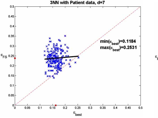
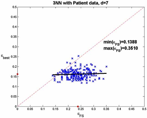
The kinds of results we observe in Table 1, lead us to ask whether it is likely that feature selection can find good feature sets. Two questions arise in the context of small samples: (1) Can one expect feature selection to yield a feature set whose error is close to that of an optimal feature set? (2) If a good feature set is not found, should it be concluded that good feature sets do not exist? These questions translate quantitatively into questions concerning conditional expectation. (1) Given the error of an optimal feature set, what is the conditionally expected error of the selected feature set? (2) Given the error of the selected feature set, what is the conditionally expected error of the optimal feature set? The first question gets directly at the question of whether one can expect suboptimal feature-selection algorithms to find good feature sets. The second question relates directly in practice because there one has a data set, applies a feature-selection algorithm, and estimates the error of the resulting classifier. If the classifier is not good, one must confront the dilemma of whether, given the data set in hand, there does not exist a feature set from which a good classifier can be designed or whether there exist feature sets from which good classifiers can be designed but the feature-selection algorithm has failed to find one. The two conditional questions have been addressed in a model-based study whose results are not promising [23]. The study also considers patient data, in which case linear regression is used as an approximation to the conditional expectation.
The patient data are those associated with Fig. (1), the complete data set consisting of the data from the 295 mi-croarrays for the 70 genes selected by [30]. The complete data set serves as the (empirical) distribution. The optimal feature set is taken from a feature-set test bed in which optimal feature sets are known [51]. Even with only 70 features, computation time is so extensive that the test bed only considers feature sets of no more than 7 genes. The regression analysis is done by drawing 200 50-point samples from the 295-point empirical distribution and applying SFFS feature selection to obtain a 7-gene feature set for each sample. We make two scatter plots, one consisting of the error pairs (εFS, εbest) and other consisting of the error pairs (εbest, εFS), where εFS and εbest are the errors for the classifiers designed on the selected feature set and best feature set, respectively, using the 50 points, and where εFS and εbest are computed using the 245 points not included in the sample. We observe in Fig. (10) (and in other approaches to choosing potential patient feature sets [23]) that feature selection does not achieve good results. In part (a) of the figure the regression of εFS on εbest is well above the 45 degree line, and the dots, marking the means, show that the mean value of εFS is approximately 0.08 greater than the mean value of εbest. The regression of εbest on εFS in the second part of the figure is even more striking, with the regression line being almost horizontal. Clearly, one cannot say much about the best feature set from the one selected. These poor results when selecting 7 features out of 70 do not bode well for achieving good results when tackling the much harder problem of selecting 10 or 20 genes out of 10,000 genes.
Fig. (10).
Linear regression for feature selection: (a) error of selected set regressed on best set; (b) error of best set regressed on selected set.
9.5. Performance of Feature-Selection Algorithms
A host of feature-selection algorithms has been proposed in the literature. When confronted with a new feature-selection algorithm, one naturally asks about its performance. This is the issue confronted in Section 9.4, where we were concerned with the regression of the error of the optimal feature set on the error of the selected feature set, or vice versa. A raw measure of feature-selection performance is given by the difference, E[εFS] − E[εbest], between the expected errors of the selected and best feature sets. This difference constitutes algorithm goodness. Without knowing it, one really cannot address the performance issue. It is important to note that performance depends on the feature-label distribution, classification rule, and the parameter settings within the feature-selection algorithm itself. For instance, if one uses SFS with bolstered resubstitution within the SFS algorithm, as we have seen, performance is different than if we use leave-one-out cross-validation within the SFS algorithm.
We are confronted by two issues when computing E[εFS] −E[εbest]: (1) we need to know an optimal feature set; and (2) we need to evaluate the errors of the classifiers corresponding to the selected and optimal feature sets. The second requirement means that we need to either know the feature-label distribution or have a sufficiently large amount of data to assure us of accurate error estimates. The first requirement is more challenging. For a model-based analysis, one must either use a model for which an optimal feature set is known, the approach taken in Section 9.3, or one must perform an exhaustive search of all possible feature sets of a given size to find one with minimum error. If one is going to use empirical data, then the sample must be sufficiently large for accurate error estimation and one must perform an exhaustive search of all possible feature sets using the empirical data as an (empirical) probability distribution to find an optimal feature set. This is the approach taken in Section 9.4 where we used a feature-selection test bed based upon good and bad prognosis breast-cancer data [51].
If one simply wants to compare the performances of two feature-selection algorithms, then one needs to compare the expected errors of the feature sets found by the two algorithms. This only presents us with the second of the preceding two requirements: evaluate their errors.
Suppose one applies the following experimental protocol: propose a new feature-selection algorithm, use it to find feature sets and the corresponding classifiers on some small data sets, use a training-data error estimator to estimate the errors of the classifiers, and then compare these errors to errors arising from another feature-selection algorithm applied in the same manner. What then can be validly concluded? First, since E[εFS] −E[εbest] is not estimated (an optimal feature-set not even being known), there is no quantitative measure of performance relative to an optimal feature set. Second, the comparison is itself not valid unless the differences in performance are sufficiently large to overcome the variance in the error estimation, perhaps with a hypothesis test, or an analysis of variance if a collection of feature-selection algorithms is to be compared. Even if the latter is accomplished, it is only valid for the empirical data on which the comparison is based. Hence, one must be very cautious when applying the obtained conclusion to any future data.
10. CLUSTERING
Clustering has become a popular data-analysis technique in genomic studies using gene-expression microarrays [52]. Time-series clustering groups together genes whose expression levels exhibit similar behavior through time. Similarity indicates possible co-regulation. Another way to use expression data is to take expression profiles over various tissue samples, and then cluster these samples based on the expression levels for each sample. This approach is used to indicate the potential to discriminate pathologies based on their differential patterns of gene expression. Admittedly, clustering has an intuitive appeal. However, the history of clustering and its historical ad hoc formulation absent a formal probabilistic setting should make a scientist extremely wary. The lack of such a formal theory opens up the potential for subjectivity, which is an anathema to science. Jain, Murty, and Flynn make this clear when writing on the classical interpretation, “Clustering is a subjective process; the same set of data items often needs to be partitioned differently for different applications” [53]. If so, then it cannot be a medium for scientific knowledge.
As discussed previously, classification achieves its scientific status in terms of a model in which quantitative statements can be made concerning classifier error. In particular, classifier error, the measure of its predictive capability, can be estimated under the assumption that the sample data come from a feature-label distribution. Until recently, clustering had not been placed into a probabilistic framework in which predictive accuracy is rigorously formulated. Many so-called “validation indices” have been proposed for evaluating clustering results; however, these tend to be significantly different than for classification validation, where the error of a classifier is given by the probability of an erroneous decision. In fact, the whole notion of “validation” as has been often used in clustering does not necessarily refer to scientific validation, as does error estimation in classification.
The scientific content of a cluster operator lies in its ability to predict results, and this ability is not determined by a single empirical event. The key to a general probabilistic theory of clustering is to recognize that classification theory is based on operators on random variables, and that the theory of clustering needs to be based on operators on random point sets. The predictive capability of a clustering algorithm must be measured by the decisions it yields regarding the partitioning of random point sets, as its decisions are compared to the underlying process from which the clusters are generated.
Using a model-based approach and a probabilistic theory of clustering as operators on random sets, we assume the points to be clustered belong to a realization of a labeled point process, and define a cluster algorithm, also called a label operator, as a mapping that assigns to every set a label function [54]. K-means, hierarchical, fuzzy C-means, self-organizing maps, and other algorithms, together with their different parameters, are different label operators. In this context, the error of a clustering algorithm is given in terms of the expected error of the label operator, the latter being the expected number of points labeled differently by it and the random process.
To rigorously quantify the notion of clustering error, suppose IA(x) denotes the index of the cluster to which a vector x belongs for the partition CA. Then the measure of disagreement (or error) between two partitions CA and CB is defined as the proportion of objects that belong to different clusters, namely,
| 16 |
where |·|indicates the number of elements of a set and n is the total number of points. Since the disagreement between two partitions should not depend on the indices used to label their clusters, the error rate is defined by
| 17 |
over all of the possible permutations π of the sets in CB. If CA is the partition of a set generated by the random process under consideration and C B is the result of cluster operator ζ, then ε∗(CA, CB) is the empirical error of ζ for that set. The error, εG[ζ], of ζ is the expected error, E[ε∗(C A, CB)], over point sets generated by the random process G [54].
The characterization of classifier model validity goes over essentially unchanged to cluster-operator model validity. A cluster-operator model is a pair M = (ζ, εε) composed of a function ζ that operates on finite point sets in and a real number εζ∈[0, 1]. For any finite point set is a partition of P. The mathematical form of the model is abstract, with εζ not specifying an actual error probability corresponding to ζ. M becomes a scientific model when it is applied to a random labeled point set. The model is valid for the random point set to the extent that εζ approximates εG[ζ]. As with classification, one can also consider the validity of the model M = (ζ, εζ) under the assumption that ζ and εζ have been arrived at via the rule model L = (Z, Ξ), where Z is a procedure to design the cluster operator ζ and Ξ is an error estimation procedure. Historically, cluster operators have not been learned from data, but they can be [54]. Here we consider error estimation. In complete analogy to classification, cluster operator ζ is better than cluster operator ξ relative to the point process G if εG[ζ] < εG[ζ].
To estimate the error of a cluster operator, ζ, we can proceed in the following manner: a sample of point sets is generated from the random set, the algorithm is applied to each point set and the clusters are evaluated relative to the known partition according to the distribution of the random point set, and the errors are averaged over the point sets composing the sample [55]. This is analogous to estimating the error of a classifier on a sample of points generated from the feature-label distribution. The resulting cluster operator model, , possesses excellent validity if the sample size is large, meaning that a large number of point sets are generated from the random set.
The foregoing distributional approach can assess the worth of a clustering algorithm in various model contexts; however, it cannot be used if one has a single collection of point data to cluster. Just as procedures for estimating classifier error from experimental data have been developed, research remains to be done on estimating clustering error. The latter presents a much more difficult problem because, whereas in the context of classification a single data set represents many realizations of the feature-label vector, for clustering one labeled data set only represents a single realization, and the data are often unlabeled.
11. VALIDATION INDICES
As historically considered, a clustering validity index evaluates clustering results based on a single realization of the random point set. Assessing the validity of a cluster operator on a single point set is analogous to assessing the validity of a classifier with a single point. Going further, assessing its validity on a single point set without knowledge of the true partition is analogous to assessing the validity of a classifier with a single unlabeled point. But there is a difference: the output of a cluster operator is a partition of a point set and therefore one can define measures for different aspects of the spatial structure of the output, for instance, compactness. One can also consider the effects of the cluster operator on subsets of the data. It could then be hoped that such measures can be used to assess the validity of the algorithm. Aside from any heuristic reasoning that might be involved in designing a validity index, the single critical point is clear: if a validity index is to assess validity, then it should be closely related to the error rate of the cluster operator. Thus, it is natural to investigate validity measures relative to how well they correlate with error rates across clustering algorithms and random-point-set models [56]. Here we describe the methodology of the investigation and give some illustrative results for point processes, clustering algorithms, and validation indices, there being a much larger collection of results reported in [56].
We report results for three models: (1) a 10-dimensional mixture of two spherical Gaussians; (2) a 2-dimensional mixture of a spherical Gaussian and a circular distribution; and (3) a 2-dimensional mixture of four spherical Gaussian distributions. Fig. (11) shows realizations of these models, where the graph for the first model is a 3D PCA plot. We consider four clustering algorithms: k-means (km), fuzzy c-means (fcm), hierarchical with Euclidean distance and complete linkage (hi[eu, co]), and hierarchical with Euclidean Fig. (11). Realizations of point processes: (a) Model 1, the 3D PCA plot for two 10-dimensional spherical Gaussians; (b) Model 2, a 2-dimensional spherical Gaussian and a circular distribution; (c) Model 3, four 2-dimensional spherical Gaussians. distance and single linkage (hi[eu, si]). Since these are well-known, we leave their description to the literature. We consider several validation indices representing the three common categories of validation indices: external, internal, and relative.
Fig. (11).
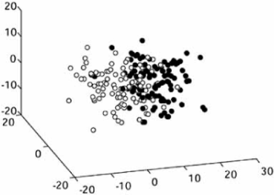
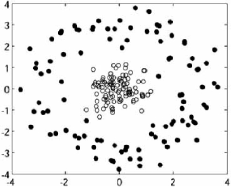
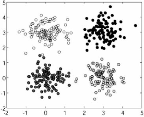
Realizations of point processes: (a) Model 1, the 3D PCA plot for two 10-dimensional spherical Gaussians; (b) Model 2, a 2-dimensional spherical Gaussian and a circular distribution; (c) Model 3, four 2-dimensional spherical Gaussians.
External validation methods are based on how pairs of points are commonly and uncommonly clustered by a cluster operator and a given partitioning, which is usually based on prior domain knowledge or some heuristic, but could in principle be based on distributional knowledge. Suppose that PG and PA are the given and algorithm-generated partitions, respectively, for the sample data S. Define four quantities: a is the number of pairs of points in S such that the pair belongs to the same class in PG and the same class in PA; b is the number of pairs such that the pair belongs to the same class in PG and different classes in PA; c is the number of pairs such that the pair belongs to different classes in PG and the same class in PA; and d is the number of pairs S such that the pair belongs to different classes in PG and different classes in PA. If the partitions match exactly, then all pairs are either in the a or d classes. The Jaccard coefficient is defined by
| 18 |
The practical problem with the external approach is that if one knows the correct partition, then the true error can be computed, and if some heuristic is used, then the measure is relative to the quality of the heuristic.
Internal validation methods evaluate the clusters based solely on the data, without external information. Typically, a heuristic measure is defined to indicate the goodness of the clustering. A common heuristic for spatial clustering is that, if the algorithm produces tight clusters and cleanly separated clusters, then it has done a good job clustering. The Dunn index is based on this heuristic. Let C = {C1, C2,..., Ck}be a partition of the n points into k clusters, δ(Ci, Cj) be a between-cluster distance, and σ(Ci) be a measure of cluster dispersion. The Dunn index is defined by
| 19 |
[57]. High values are favorable. As defined, the index leaves open the distance and dispersion measures, and different ones have been employed. Here we utilize the centroids of the clusters: summation
| 20 |
where and are the centroids of Ci and Cj, respectively; and
| 21 |
Relative validation methods are based on the measurement of the consistency of the algorithms, comparing the clusters obtained by the same algorithm under different conditions. Here we consider the stability index, which assesses the validity of the partitioning found by clustering algorithms [58, 59]. The stability index measures the ability of a clustered data set to predict the clustering of another data set sampled from the same source. Let us assume that there exists a partition of a set S of n objects into K groups, C = {C1,…, CK}, and a partition of another set S0 of n0 objects into K0 groups, C0 = {C01,… , C0K0}. Let the labels α and α0 0K0 be defined by α(x) = i if x є Ci, for x α S, and α0(x) = i if x є C0i, for xєS0, respectively. The labeled set (S, α) can be used to train a classifier that induces a labeling α∗ on S0 by α∗(x) = f (x). The consistency of the pairs (S, α) and (S0, α0) is measured by the similarity between the original labeling α0 and the induced labeling α∗ in S0:
| 22 |
over all possible permutation of the labels for where
| 23 |
with δ(u, v) = 0 if u = v and δ(u , v) = 1 if u ≠ v. The stability for a clustering algorithm is defined by the expectation of the stability for pairs of sets drawn from the same source:
| 24 |
In practice, there is only one set S of points with which to estimate the stability of a clustering algorithm. Estimation of the stability is obtained via a re-sampling scheme [58]: the set S is partitioned in two disjoint subsets, S1 and S2, the clustering algorithm is applied to obtain two partitions, C 1 and is computed, and the process is repeated and the values averaged to obtain an estimate ofζ . We evaluate the goodness of a validity index by computing Kendall’s rank correlation between the error of the clustering algorithm and the validity index. This correlation is estimated using 100 generated data sets in each case and averaging. The external Jaccard coefficient is computed using the true partition. The results are given in Table 2. Overall, both in the few examples presented here and the full analysis [56], the results raise serious questions concerning the scientific validity of validity indices. Even in model 1, with two Gaussians, the internal Dunn index does not perform well. The stability index performs poorly in all cases except for two clustering algorithms with model 3, but even here performs very poorly for k-means and single-linkage hierarchical clustering. The Jaccard coefficient, using the (in practice, unknown) true partitions, has problems with hierarchical clustering. This study reveals that there are serious validity issues when using standard clustering algorithms: if the validity indices cannot be trusted, and these constitute the standard way of assessing validity, then what scientific meaning can be attributed to the results of clustering algorithms?
Table 2.
Kendall’s Correlation Between Validity Indices and Clustering Error
| Model 1 | Model 2 | Model 3 | |||||||
|---|---|---|---|---|---|---|---|---|---|
| Jaccard | Dunn | Stability | Jaccard | Dunn | Stability | Jaccard | Dunn | Stability | |
| km | 0.91 | 0.63 | 0.62 | 0.84 | 0.17 | 0.19 | 0.88 | 0.78 | 0.37 |
| fcm | 0.99 | 0.63 | 0.65 | 0.89 | 0.04 | 0.29 | 0.99 | 0.80 | 0.83 |
| hi[eu,co] | 0.36 | 0.40 | 0.39 | 0.63 | 0.01 | 0.26 | 0.94 | 0.77 | 0.81 |
| hi[eu,si] | 0.95 | 0.57 | 0.55 | 0.19 | 0.56 | 0.35 | 0.39 | 0.40 | 0.38 |
12. CONCLUDING REMARKS
We re-iterate what we said in the Introduction: much more attention needs to be paid to the validation of methods using in genomics. Sound science requires conclusions to be drawn only when conclusions are warranted. Whether or not a conclusion is warranted can only be answered within the framework of a sound epistemology – and this means rigorous validation. There is no nonmathematical way to precisely describe knowledge regarding model validity. It depends on the choice of validity measurement and the mathematical properties of that measurement as applied in different circumstances. In all cases, the nature of our knowledge rests with the mathematical theory we have concerning the measurements. That cannot be simplified. If either the available theory or one’s familiarity with the theory is limited, then one’s appreciation of the scientific content of a model is limited.
Fig. (7).
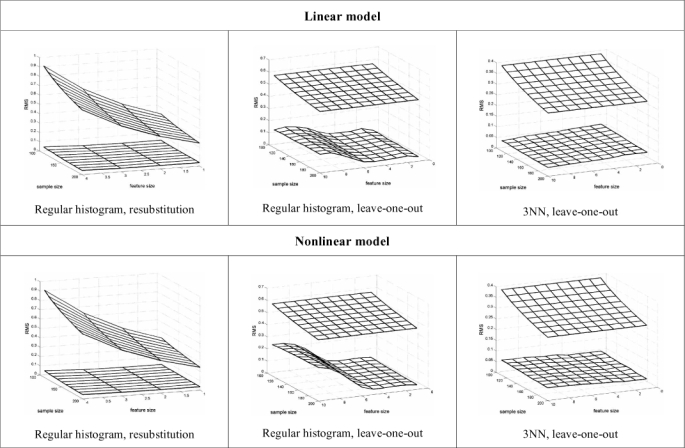
Comparison of the true RMS values (lower plane in each plot) with the universal RMS bounds (upper plane in each plot).
ACKNOWLEDGEMENTS
We would like to acknowledge the National Science Foundation (CCF-0514644), the National Human Genome Research, and the Translational Genomics Research Institute for supporting much of the work behind this paper.
REFERENCES
- 1.Garrod AE. The incidence of alkaptonuria: a study in chemical individuality. Lancet. 1902;2:1616–1620. [PMC free article] [PubMed] [Google Scholar]
- 2.Garrod AE. Inborn errors of metabolism. London: H. Frowde, Hodder & Stoughton; 1923. [Google Scholar]
- 3.Lejeune J, Gautier M, Turpin R. Study of somatic chromosomes from 9 mongoloid children. C R Hebd Seances Acad Sci. 1959;248:1721–1722. [PubMed] [Google Scholar]
- 4.Nowell PC, Hungerford DA. A minute chromosome in human chronic granulocytic leukemia. Science. 1960;132:1497. doi: 10.1126/science.144.3623.1229. [DOI] [PubMed] [Google Scholar]
- 5.Goyette MC, Cho K, Fasching CL, Levy DB, Kinzler KW, Paraskeva C, Vogelstein B, Stanbridge EJ. Progression of colorectal cancer is associated with multiple tumor suppressor gene defects but inhibition of tumorigenicity is accomplished by correction of any single defect via chromosome transfer. Mol Cell Biol. 1992;12:1387–1395. doi: 10.1128/mcb.12.3.1387. [DOI] [PMC free article] [PubMed] [Google Scholar]
- 6.Perou CM, Sorlie T, Eisen MB, van de Rijn M, Jeffrey SS, Rees CA, Pollack JR, Ross DT, Johnsen H, Akslen LA, Fluge O, Pergamenschikov A, Williams C, Zhu SX, Lonning PE, Borresen-Dale AL, Brown PO, Botstein D. Molecular portraits of human breast tumours. Nature. 2000;406:747–752. doi: 10.1038/35021093. [DOI] [PubMed] [Google Scholar]
- 7.van ’t Veer LJ, Dai H, van de Vijver MJ, He YD, Hart AA, Bernards R, Friend SH. Expression profiling predicts outcome in breast cancer. Breast Cancer Res. 2003;5:57–58. doi: 10.1186/bcr562. [DOI] [PMC free article] [PubMed] [Google Scholar]
- 8.Gidalevitz T, Ben-Zvi A, Ho KH, Brignull HR, Morimoto RI. Progressive disruption of cellular protein folding in models of polyglutamine diseases. Science. 2006;311:1471–1474. doi: 10.1126/science.1124514. [DOI] [PubMed] [Google Scholar]
- 9.Kaneta Y, Kagami Y, Tsunoda T, Ohno R, Nakamura Y, Katagiri T. Genome-wide analysis of gene-expression profiles in chronic myeloid leukemia cells using a cDNA microarray. Int J Oncol. 2003;23:681–691. [PubMed] [Google Scholar]
- 10.Mao R, Wang X, Spitznagel EL, Jr, Frelin LP, Ting JC, Ding H, Kim JW, Ruczinski I, Downey TJ, Pevsner J. Primary and secondary transcriptional effects in the developing human Down syndrome brain and heart. Genome Biol. 2005;6:R107. doi: 10.1186/gb-2005-6-13-r107. [DOI] [PMC free article] [PubMed] [Google Scholar]
- 11.Alizadeh AA, Eisen MB, Davis RE, Ma C, Lossos IS, Rosenwald A, Boldrick JC, Sabet H, Tran T, Yu X, Powell JI, Yang L, Marti GE, Moore T, Hudson J, Jr, Lu L, Lewis DB, Tibshirani R, Sherlock G, Chan WC, Greiner TC, Weisenburger DD, Armitage JO, Warnke R, Levy R, Wilson W, Grever MR, Byrd JC, Botstein D, Brown PO, Staudt LM. Distinct types of diffuse large B-cell lymphoma identified by gene expression profiling. Nature. 2000;403:503–511. doi: 10.1038/35000501. [DOI] [PubMed] [Google Scholar]
- 12.Khan J, Wei JS, Ringner M, Saal LH, Ladanyi M, Westermann F, Berthold F, Schwab M, Antonescu CR, Peterson C, Meltzer PS. Classification and diagnostic prediction of cancers using gene expression profiling and artificial neural networks. Nat Med. 2001;7:673–679. doi: 10.1038/89044. [DOI] [PMC free article] [PubMed] [Google Scholar]
- 13.Hedenfalk I, Duggan D, Chen Y, Radmacher M, Bittner M, Simon R, Meltzer P, Gusterson B, Esteller M, Kallioniemi OP, Wilfond B, Borg A, Trent J, Raffeld M, Yakhini Z, Ben-Dor A, Dougherty E, Kononen J, Bubendorf L, Fehrle W, Pittaluga S, Gruvberger S, Loman N, Johannsson O, Olsson H, Sauter G. Gene-expression profiles in hereditary breast cancer. N Engl J Med. 2001;344:539–548. doi: 10.1056/NEJM200102223440801. [DOI] [PubMed] [Google Scholar]
- 14.Monti S, Savage KJ, Kutok JL, Feuerhake F, Kurtin P, Mihm M, Wu B, Pasqualucci L, Neuberg D, Aguiar RC, Dal Cin P, Ladd C, Pinkus GS, Salles G, Harris NL, Dalla-Favera R, Habermann TM, Aster JC, Golub TR, Shipp MA. Molecular profiling of diffuse large B-cell lymphoma identifies robust subtypes including one characterized by host inflammatory response. Blood. 2005;105:1851–1861. doi: 10.1182/blood-2004-07-2947. [DOI] [PubMed] [Google Scholar]
- 15.Gruvberger S, Ringner M, Chen Y, Panavally S, Saal LH, Borg A, Ferno M, Peterson C, Meltzer PS. Estrogen receptor status in breast cancer is associated with remarkably distinct gene expression patterns. Cancer Res. 2001;61:5979–5984. [PubMed] [Google Scholar]
- 16.Allander SV, Nupponen NN, Ringner M, Hostetter G, Maher GW, Goldberger N, Chen Y, Carpten J, Elkahloun AG, Meltzer PS. Gastrointestinal stromal tumors with KIT mutations exhibit a remarkably homogeneous gene expression profile. Cancer Res. 2001;61:8624–8628. [PubMed] [Google Scholar]
- 17.Dave SS, Wright G, Tan B, Rosenwald A, Gascoyne RD, Chan WC, Fisher RI, Braziel RM, Rimsza LM, Grogan TM, Miller TP, LeBlanc M, Greiner TC, Weisenburger DD, Lynch JC, Vose J, Armitage JO, Smeland EB, Kvaloy S, Holte H, Delabie J, Connors JM, Lansdorp PM, Ouyang Q, Lister TA, Davies AJ, Norton AJ, Muller-Hermelink HK, Ott G, Campo E, Montserrat E, Wilson WH, Jaffe ES, Simon R, Yang L, Powell J, Zhao H, Goldschmidt N, Chiorazzi M, Staudt LM. Prediction of survival in follicular lymphoma based on molecular features of tumor-infiltrating immune cells. N Engl J Med. 2004;351:2159–2169. doi: 10.1056/NEJMoa041869. [DOI] [PubMed] [Google Scholar]
- 18.Dougherty ER. Small Sample Issues for Microarray-Based Classification. Comparative and Functional Genomics. 2001;2:28–34. doi: 10.1002/cfg.62. [DOI] [PMC free article] [PubMed] [Google Scholar]
- 19.Vapnik VN, Chervonenkis A. On the Uniform Convergence of Relative Frequencies of Events to Their Probabilities. Theory of Probability and its Applications. 1971;16:264–280. [Google Scholar]
- 20.Braga-Neto UM, Dougherty ER. Is Cross-Validation Valid for Small-Sample Microarray Classification. Bioinformatics. 2004;20:374–380. doi: 10.1093/bioinformatics/btg419. [DOI] [PubMed] [Google Scholar]
- 21.Molinaro AM, Simon R, Pfeiffer RM. Prediction Error Estimation: A Comparison of Resampling Methods. Bioinformatics. 2005;21:3301–3307. doi: 10.1093/bioinformatics/bti499. [DOI] [PubMed] [Google Scholar]
- 22.Sima C, Attoor S, Braga-Neto UM, Lowey J, Suh E, Dougherty ER. Impact of Error Estimation on Feature-Selection Algorithms. Pattern Recognition. 2005;38:2472–2482. [Google Scholar]
- 23.Sima C, Dougherty ER. What Should Be Expected from Feature Selection in Small-Sample Settings. Bioinformatics. 2006;22:2430–2436. doi: 10.1093/bioinformatics/btl407. [DOI] [PubMed] [Google Scholar]
- 24.Zhou X, Mao KZ. The Ties Problem Resulting from Counting-Based Error Estimators and Its Impact on Gene Selection Algorithms. Bioinformatics. 2006;22:2507–2515. doi: 10.1093/bioinformatics/btl438. [DOI] [PubMed] [Google Scholar]
- 25.Dougherty ER, Braga-Neto U. Epistemology of Computational Biology: Mathematical Models and Experimental Prediction as the Basis of Their Validity. Biol Syst. 2006;14:65–90. [Google Scholar]
- 26.Kauffman SA. Metabolic stability and epigenesis in randomly constructed genetic nets. Theoretical Biol. 1969;22:437–467. doi: 10.1016/0022-5193(69)90015-0. [DOI] [PubMed] [Google Scholar]
- 27.Kauffman SA. Homeostasis and differentiation in random genetic control networks. Nature. 1969;224:177–178. doi: 10.1038/224177a0. [DOI] [PubMed] [Google Scholar]
- 28.Mehta T, Murat T, Allison DB. Towards sound epistemological foundations of statistical methods for high-dimensional biology. Nat Genet. 2004;36:943–947. doi: 10.1038/ng1422. [DOI] [PubMed] [Google Scholar]
- 29.van de Vijver MJ, He YD, van’t Veer LJ, Dai H, Hart AA, Voskuil DW, Schreiber GJ, Peterse JL, Roberts C, Marton MJ, Parrish M, Atsma D, Witteveen A, Glas A, Delahaye L, van der Velde T, Bartelink H, Rodenhuis S, Rutgers ET, Friend SH, Bernards R. Gene Expression Signature as a Predictor of Survival in Breast Cancer. N Engl J Med. 2002;347:1999–2009. doi: 10.1056/NEJMoa021967. [DOI] [PubMed] [Google Scholar]
- 30.van’t Veer LJ, Dai H, van de Vijver MJ, He YD, Hart AAM, Mao M, Peterse HL, van der Kooy K, Marton MJ, Witteveen AT, Schreiber GJ, Kerkhoven RM, Roberts C, Linsley PS, Bernards R, Friend SH. Gene Expression Profiling Predicts Clinical Outcome of Breast Cancer. Nature. 2002;415:530–536. doi: 10.1038/415530a. [DOI] [PubMed] [Google Scholar]
- 31.Braga-Neto UM. Fads and Fallcies in the Name of Small-Sample Microarray Classification. IEEE Signal Processing Magazine. 2007 [Google Scholar]
- 32.Kobayashi T, Yamaguchi M, Kim S, Morikawa J, Ueno S, Suh E, Dougherty ER, Shmulevich I, Shiku H, Zhang W. Gene Expression Profiling Identifies Strong Feature Genes that Classify de novo CD5+ and CD5_ Diffuse Large B-cell Lymphoma and Mantle Cell Lymphoma. Cancer Res. 2003;63:60–66. [PubMed] [Google Scholar]
- 33.Devroye L, Gyorfi L, Lugosi G. A Probabilistic Theory of Pattern Recognition. New York: Springer-Verlag; 1996. [Google Scholar]
- 34.Braga-Neto UM, Dougherty ER. Exact Performance of Error Estimators for Discrete Classifiers. Pattern Recognition. 2005;38:1799–1814. [Google Scholar]
- 35.Efron B. Bootstrap Methods: Another Look at the Jacknife. Annals of Statistics. 1979;7:1–26. [Google Scholar]
- 36.Efron B. The Jacknife, The Bootstrap, and Other Resampling Plans. SIAM NSF-CBMS, monograph #38. 1983 [Google Scholar]
- 37.Sima C, Dougherty ER. Optimal Convex Error Estimators for Classification. Pattern Recognition. 2006;39:1763–1780. [Google Scholar]
- 38.Braga-Neto UM, Dougherty ER. Bolstered Error Estimation. Pattern Recognition. 2004;37:1267–1281. [Google Scholar]
- 39.Xu Q, Hua J, Braga-Neto UM, Xiong Z, Suh E, Dougherty ER. Confidence Intervals for the True Classification Error Conditioned on the Estimated Error. Technology in Cancer Research and Treatment. 2006;5:579–590. doi: 10.1177/153303460600500605. [DOI] [PubMed] [Google Scholar]
- 40.Devroye L, Wagner T. Distribution-free Inequalities for the Deleted and Hold-out Error Estimates. IEEE Transactions on Information Theory. 1979;25:202–207. [Google Scholar]
- 41.Sima C, Braga-Neto UM, Dougherty ER. Superior Feature-Set Ranking For Small Samples Using Bolstered Error Estimation. Bioinformatics. 2005;21:1046–1054. doi: 10.1093/bioinformatics/bti081. [DOI] [PubMed] [Google Scholar]
- 42.Braga-Neto UM, Hashimoto R, Dougherty ER, Nguyen DV, Carroll RJ. Is Cross-validation Better than Resubstitution for Ranking Genes. Bioinformatics. 2004;20:253–258. doi: 10.1093/bioinformatics/btg399. [DOI] [PubMed] [Google Scholar]
- 43.Hughes GF. On the Mean Accuracy of Statistical Pattern Recognizers. IEEE Transactions on Information Theory. 1968;14:55–63. [Google Scholar]
- 44.Jain AK, Chandrasekaran B. Dimensionality and Sample Size Considerations in Pattern Recognition Practice. In: Krishnaiah PR, Kanal LN, editors. Classification, Pattern Recognition and Reduction of Dimensionality. Vol. 2. Amsterdam: North-Holland; 1982. pp. 835–856. (Handbook of Statistics). [Google Scholar]
- 45.Hua J, Xiong Z, Dougherty ER. Determination of the Optimal Number of Features for Quadratic Discriminant Analysis Via the Normal Approximation to the Discriminant Distribution. Pattern Recognition. 2005;38:403–421. [Google Scholar]
- 46.Hua J, Xiong Z, Lowey J, Suh E, Dougherty ER. Optimal Number of Features as a Function of Sample Size for Various Classification Rules. Bioinformatics. 2005;21:1509–1515. doi: 10.1093/bioinformatics/bti171. [DOI] [PubMed] [Google Scholar]
- 47.Cover T, van Campenhout J. On the Possible Orderings in the Measurement Selection Problem. IEEE Transasctions on Systems, Man, and Cybernetics. 1977;7:657–661. [Google Scholar]
- 48.Pudil P, Novovicova J, Kittler J. Floating Search Methods in Feature Selection. Pattern Recognition Lett. 1994;15:1119–1125. [Google Scholar]
- 49.Jain AK, Zongker D. Feature Selection: Evaluation, Application, and Small Sample Performance. IEEE Transactions on Pattern Analysis and Machine Intelligence. 1997;19:153–158. [Google Scholar]
- 50.Kudo M, Sklansky J. Comparison of Algorithms that Select Features for Pattern Classifiers. Pattern Recognition. 2000;33:25–41. [Google Scholar]
- 51.Choudhary A, Brun M, Hua J, Lowey J, Suh E, Dougherty ER. Genetic Test Bed for Feature Selection. Bioinformatics. 2006;22:837–842. doi: 10.1093/bioinformatics/btl008. [DOI] [PubMed] [Google Scholar]
- 52.Ben-Dor A, Shamir R, Yakhini Z. Clustering Gene Expression Patterns. Computational Biology. 1999;6:281–297. doi: 10.1089/106652799318274. [DOI] [PubMed] [Google Scholar]
- 53.Jain AK, Murty MN, Flynn PJ. Data Clustering: A Review. ACM Computer Surveys. 1999;31:264–323. [Google Scholar]
- 54.Dougherty ER, Brun M. A Probabilistic Theory of Clustering. Pattern Recognition. 2004;37:917–925. [Google Scholar]
- 55.Dougherty ER, Barrera J, Brun M, Kim S, Cesar RM, Chen Y, Bittner ML, Trent JM. Inference From Clustering With Application to Gene-Expression Microarrays. Comput Biol. 2002;9:105–126. doi: 10.1089/10665270252833217. [DOI] [PubMed] [Google Scholar]
- 56.Brun M, Sima C, Hua J, Lowey J, Carroll B, Suh E, Dougherty ER. Model-Based Evaluation of Clustering Validation Measures. Pattern Recognition. 2007;40:807–824. [Google Scholar]
- 57.Dunn JC. A Fuzzy Relative of the ISODATA Process and Its Use in Detecting Well-Separated Clusters. Cybernetics. 1973;3:32–57. [Google Scholar]
- 58.Lange T, Braun M, Roth V, Buhmann JM. Stability-based Model Selection. Advances in Neural Information Processing Systems. 2002 [Google Scholar]
- 59.Roth V, Braun M, Lange T, Buhmann JM. Artificial Neural Networks - ICANN. Berlin: Springer; 2002. Stability-based Model Order Selection in Clustering with Application to Gene Expression Data; pp. 607–612. [Google Scholar]