Compressed Sensing for Resolution Enhancement of Hyperpolarized ¹³C Flyback 3D-MRSI

Abstract

High polarization of nuclear spins in liquid state through dynamic nuclear polarization has enabled the direct monitoring of ¹³C metabolites in vivo at very high signal to noise, allowing for rapid assessment of tissue metabolism. The abundant SNR afforded by this hyperpolarization technique makes high resolution ¹³C 3D-MRSI feasible. However, the number of phase encodes that can be fit into the short acquisition time for hyperpolarized imaging limits spatial coverage and resolution. To take advantage of the high SNR available from hyperpolarization, we have applied compressed sensing to achieve a factor of 2 enhancement in spatial resolution without increasing acquisition time or decreasing coverage. In this paper, the design and testing of compressed sensing suited for a flyback ¹³C 3D-MRSI sequence are presented. The key to this design was the undersampling of spectral k-space using a novel blipped scheme, thus taking advantage of the considerable sparsity in typical hyperpolarized ¹³C spectra. Phantom tests validated the accuracy of the compressed sensing approach and initial mouse experiments demonstrated in vivo feasibility.

1. Introduction

Carbon-13 spectroscopy has traditionally been limited by low signal strength. With the development of techniques to maintain hyperpolarization of carbon-13 in liquid state [1], it has become possible to use ¹³C substrates (tracers) for medical imaging [2]. More recent studies have used the metabolically active substrate [l-¹³C]pyruvate to examine its conversion to [l-¹³C]lactate, [l-¹³C]alanine, and ¹³C-bicarbonate [3–5]. Spectroscopic examination of these metabolic pathways in the presence and absence of disease has enormous diagnostic potential. Specifically, it has already been shown that the levels of ¹³C metabolic products differ between disease and non-disease states in a mouse model of prostate cancer [5]. As pointed out in [5], partial voluming may complicate the interpretation of non-disease spectra because of the small size of the normal mouse prostate. With the abundant SNR available in hyperpolarized studies, it would be beneficial to sacrifice some signal for improved spatial resolution, but the time limitation imposed by T1 relaxation severely restricts the possible number of phase encode steps.

Recent advances in mathematical theory have opened the door for accurate reconstruction of sparse signals from sub-nyquist sampling [6–7]. Less technical descriptions from the same authors, focusing on the practical limits of compressed sensing, have shown reconstructions from realistic data sets [8–9]. In addition, Lustig et al, in an exposition of the application of compressed sensing to MRI, shows that many MR images exhibit a high degree of sparsity and provides high quality proof of concept results drawn from multi-slice fast spin-echo brain imaging and 3DFT time of flight contrast enhanced angiography [10]. Lustig lists three criteria for the successful application of compressed sensing: 1) the data have a sparse representation in a transform domain 2) the aliasing from undersampling be incoherent in that transform domain and 3) a non-linear reconstruction be used to enforce both sparsity of data and consistency with measurements. The successes in [10], coupled with the sparsity in hyperpolarized spectra, make hyperpolarized ¹³C spectroscopic imaging a logical choice for the application of compressed sensing. In other words, for hyperpolarized ¹³C, the first criterion is satisfied by the inherent sparseness of hyperpolarized spectra, and the third criterion can be met by using the same non-linear reconstruction from [10]. The primary challenge then is to satisfy the second criterion: developing an undersampling approach to achieve suitable incoherent aliasing.

The sparsity of hyperpolarized spectra has been previously exploited for accelerated imaging [11–12] by using a priori knowledge of metabolite resonance locations and linewidths (factor of 4 acceleration reported in a phantom demonstration [11]). Compressed sensing, however, requires no assumptions except that the underlying data are sparse in some domain.

A 3D-MRSI sequence using flyback echo-planar readout gradients [13–14] provides a fast method for acquiring hyperpolarized spectra and is less sensitive to timing errors, eddy currents and B₀ inhomogeneity than EPI and spiral readout schemes, especially in vivo. This paper presents a methodology for accelerating the acquisition of hyperpolarized spectra by a factor of 2 using compressed sensing in conjunction with a modified flyback echo-planar 3D-MRSI sequence. A few initial phantom and in vivo examples are presented as proof of concept.

2. Theory

Pulse Sequence

The pulse sequence developed for this study builds on the one diagrammed in Figure 1, which is a double spin-echo sequence with a flyback echo-planar readout [14]. Details of the flyback design are given in [13]. As explained in [14], a spin-echo sequence was desired in order to mitigate the effects of B₀ inhomogeneity and allow for a full echo acquisition. Owing to its insensitivity to transmit gain, this double adiabatic sequence outperforms a conventional spin-echo sequence in preserving hyperpolarization over the repeated excitations needed for the phase encodes in an MRSI acquisition [14]. Ultimately, this sequence reads out a rectilinear k-space trajectory, with a typical result being 59×8×8×16 (k_f-k_x-k_y-k_z) 4D k-space data.

Figure 1.

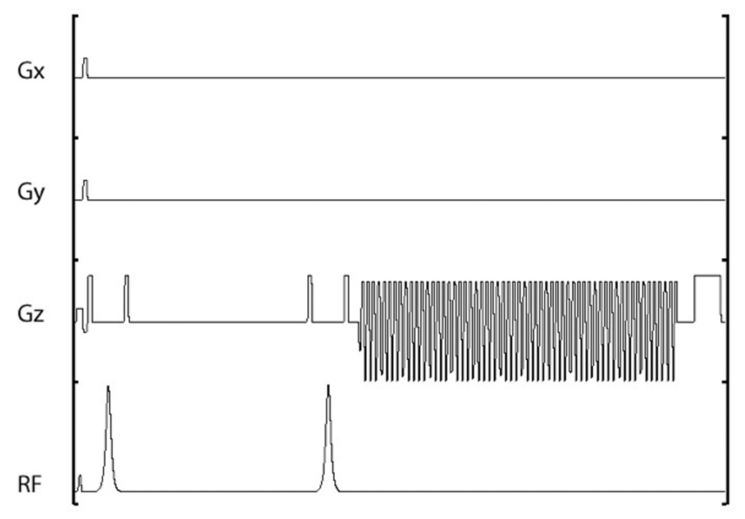
Double spin-echo sequence timing diagram. The RF consists of a small tip excitation followed by two adiabatic pulses (phase channel not shown). Phase encoding is along x and y while the 59-lobe flyback readout is along z. An echo is formed during the middle of the flyback readout with TE = 140ms.

Key Results from Compressed Sensing Literature

Fundamentally, compressed sensing claims to perfectly reconstruct sparse signals of length N from a subset of samples. For example, suppose a length N discrete signal f consists of M non-zero points. Then, with extremely high probability, f can be recovered exactly from K Fourier measurements where

$$K\ge \mathit{\text{Const}}·M\text{log}N$$ (1)

and the solution is found by solving the convex minimization problem

$$\text{min}{\displaystyle \sum _n\left|g[\mathrm{n}]\right|}s.t.F_K\{g[n]\}=y$$ (2)

where F_k is the Fourier transform evaluated at K locations and y is the set of K measured Fourier coefficients [8]. In words, Eq. [2] states that for all reconstructions g[n] whose Fourier coefficients match those at the K measured positions, the unique and correct solution is the one that minimizes the absolute sum of g, i.e. the ℓ₁ norm in the object domain. The theorems of compressed sensing are actually much more general than this concrete example suggests. In other words, the signal f only needs to be sparse in some domain, not necessarily the object domain, and the K measurements do not necessarily have to be Fourier measurements. From a practical standpoint, the application specific values for M, N, and the constant multiplier determine the feasibility of compressed sensing. Additionally, a real-world signal will never consist of just M non-zero points in any domain, but it will usually be well approximated by M sparse transform coefficients. For example, the fidelity with which compressed sensing reproduces an M-term wavelet approximation, i.e. the sparse domain being the wavelet domain, could serve as a benchmark for real-world signals such as NMR spectra [9]. For various N = 1024 test signals in [8], Candes empirically determined that for compressed sensing to match the accuracy of an M-term wavelet representation, K ≈ 3M–5M measurements were required, which was also observed in [10]. As mentioned previously, for the actual implementation of compressed sensing, the K measurements must be collected with a sampling pattern that produces incoherent aliasing in the domain, such as the wavelet domain, where the signal shows sparsity [10]. A random sampling pattern in k-space almost always meets this criterion.

At this point, it is interesting to consider the connection between compressed sensing and existing techniques in NMR, such as maximum entropy [15–16] and minimum area [17] reconstruction, used for the related problem of computation of spectra from short, noisy data records. Recently, Stern et al showed that a specific form of iterative thresholding, a technique similar to maximum entropy and minimum area reconstruction, is equivalent to the minimum ℓ₁ norm reconstruction in compressed sensing [18]. Additionally, Stern explains how ℓ₁ norm reconstruction gives insight into the performance of maximum entropy and minimum area reconstruction. Thus, compressed sensing could be viewed as a generalization of existing NMR techniques.

3D-MRSI Signal

The most straightforward application of compressed sensing to hyperpolarized 3D-MRSI would be to undersample in k_x and k_y. For example, to achieve 16×8 spatial resolution in the time of 8×8 phase encodes, i.e. a speedup factor of 2, one could simply collect 8×8 of the phase encodes in a conventional 16×8 scan (K = 64, N = 128). However, our wavelet simulations have shown that such a small N leads to a relatively large M and thus does not provide enough sparsity to exploit. A better strategy would be to attempt undersampling in the k_f and k_x dimensions, considering that typical hyperpolarized acquisitions are inherently sparse in the spectral dimension. As shown in the wavelet simulations of Figure 2, a signal of this type (spectral dimension and one spatial dimension) exhibits considerable sparsity. (Note that wavelet transforms were chosen because they do a good job of sparsifying NMR spectra [9], though other choices are possible as well.) The key point is that the majority of the sparsity occurs in the spectra and therefore the time domain should be undersampled. However, the implementation of time domain undersampling is not at all straightforward, as the next section demonstrates. A scheme to undersample in the time domain as well as in one spatial domain was employed, mainly exploiting spectral sparsity but some spatial sparsity as well.

Figure 2.

Demonstration of wavelet compressibility of a ¹³C spectroscopic signal. A row of magnitude spectra (64×16) from a 3D-MRSI phantom data set (see Figure 5 for examples of rows of spectra) was taken as the test signal. Note that the 59 spectral points from the 59 flyback lobes were zero-padded to 64 because the wavelet software we used required dyadic numbers. a) The 16 original spectra. b) A 2D Daubechies wavelet transform was applied to the 64×16 data, after which the top 10% wavelet coefficients were retained and the inverse 2D wavelet transform taken. c) The magnitude error between a) and b). Note that a), b), and c) have the same y-axis scale. The 64×16 data were reconstructed very accurately from only 10% of their wavelet coefficients, showing that the signal of interest exhibits considerable fundamental sparsity.

Implementation of k_f-k_x incoherent sampling

The key to implementing a k-space trajectory that randomly undersamples in k_f-k_x lies in the random sampling of k_f = t using blips. Figure 3 and Figure 4 illustrate a scheme that achieves k_f sub-sampling by hopping back and forth between adjacent k_x lines during a flyback readout. In this manner, data from two k_f-k_x lines are acquired during a single phase encode, in effect randomly undersampling in time. Thus, 16×8 resolution can be achieved in half the time by collecting 8×8 of the readouts in a conventional 16×8 scan. This approach is somewhat similar to the k–t sparse scheme in [19–20], but here we apply gradients to move around in k_f space instead of reordering phase encodes. This blipped scheme addresses the design challenge of generating sufficient incoherent aliasing through random undersampling, in other words meeting the second criterion for the successful application of compressed sensing. Without the blips, there would be too much structure to the undersampling, which would lead to coherent aliasing. To reiterate, the design in Figure 3 achieves two-fold undersampling by jumping between two lines. A design to achieve three-fold undersampling would have to jump between 3 lines, and a design to achieve four-fold undersampling would have to jump between 4 lines. Finally, we used the Duyn method [21–22] to measure the actual k-space trajectory traced out by our blips. As expected, on a modern clinical scanner with eddy current compensation, the measured k-space trajectory closely matched the intended one. In other words, the blips produced minimal side effects, and unintended k-space deviations were negligible.

Figure 3.

Blipped scheme for k_f-k_x sub-sampling. Top: The only modification to the pulse sequence shown in Figure 1 is the addition of blips during the rewind portions of the flyback readout. The area of each blip is the area in an x-phase encode step. Bottom: Associated order of k-space readout. A single readout now covers two k_f-k_x lines.

Figure 4.

Blipped patterns to cover 16 k_f-k_x lines, resulting coverage, and point spread function. a) Actual 8 blipped patterns used to cover 16 k_f-k_x lines in a pseudo-random manner. b) Associated k-space sampling. Because twice as much k-space is covered in the time of 8 phase encodes, half of the 59×16 k_f-k_x points are missing (missing points are black). c) 2D point spread function of pseudo-random pattern in b).

3. Experimental

Pulse Sequence and Hardware

The source code from [14], originally a free induction decay (FID) MRSI sequence, was modified to incorporate triangular gradient blips. In an attempt to minimize eddy current effects, the blips were made 0.8 ms, relatively wide considering the time between adjacent flat flyback portions was 1.16 ms. The amplitude of the blips was calculated by the source code so that each blip’s area equaled the area in a phase encode increment. As in [5], a variable flip angle (VFA) scheme [23], i.e. increasing flip angle over time to compensate for the loss in hyperpolarized signal, was used in the in vivo experiments. The actual n^th flip angle θ[n] precalculated by the source code for a given acquisition of N flips was as follows:

$$\theta [n]=\{\begin{array}{ccc}{90}^{°}\hfill & \mathit{\text{if}}\hfill & n=N\hfill \\ \text{arctan}(\text{sin}(\theta [n+1]))\hfill & \mathit{\text{if}}\hfill & n<N\hfill \end{array}$$ (3)

For example, in our acquisition with N = 8×8 = 64 readouts, θ[64] = 90°, θ[63] = arctan(sin(90°)) = 45°, θ[62] = arctan(sin(45°)) = 35.3°, … θ[1] = 7.2°. Calibration of the pulse angles was performed on the day of each study using a prescan of a corn oil phantom. In addition, for the in vivo experiments, as in [5], reordering of phase encodes to collect data near the k-space origin first was also employed. For all experiments, T2-weighted images were acquired with a fast spin-echo sequence, after which MRSI data, phase encode localized in x/y with flyback readout in the S/I direction z, were collected. All experiments were performed on a General Electric EXCITE 3T (Waukesha, WI) clinical scanner equipped with 40 mT/m, 150 mT/m/ms gradients and a broadband RF amplifier. Custom built, dual-tuned ¹H/¹³C transmit/receive coils were used for all phantom and animal experiments.

Reconstruction

For acquisitions without blipped gradients, the reconstruction procedure, carried out with custom MRSI software [24], was as follows: 1) sample the raw flyback data to obtain a 4D matrix of k-space data 2) apodize each FID and apply a linear phase correction to the spectral samples as described in [13] to account for the tilted k-space trajectory characteristic of a flyback readout and 3) perform a 4D Fourier transform with zero-padding of the spectra. For blipped acquisitions, the processing pipeline was modified in that the flyback sampling was performed in MATLAB (Mathworks Inc., Natick, MA) and the k-space points missed by the blipped trajectory were iteratively filled in using a non-linear conjugate gradient implementation of Eq. [2] [10]. Specifically, the reconstruction procedure for blipped acquisitions was as follows: 1) order the raw blipped flyback data to obtain a 4D matrix of k-space data missing half of its k_f-k_s points 2) inverse Fourier transform the fully sampled k_y and k_z dimensions 3) iteratively fill in the missing k_f-k_x points in the 4D matrix using the algorithm from [10] 4) forward Fourier transform the k_y and k_z dimensions to put the data back into the form of a filled k_f-k_x-k_y-k_z set 5) apodize each FID and apply a linear phase correction and 6) perform a 4D Fourier transform with zero-padding of the spectra. Transforming in the fully sampled k_y and k_z dimensions allowed us to separate the multi-dimensional reconstruction problem into many separable 2D reconstructions, reducing the memory requirements and allowing parallel processing as was done for the 3D angiography example in [10]. The total reconstruction time for the normal and compressed sensing reconstructions were ~5 seconds and ~20 minutes respectively on a 1 GHz, 2 GB RAM Sun workstation running Red Hat Linux. The compressed sensing reconstruction was implemented in MATLAB. We expect significant speed improvement with code optimization.

Phantom

Experiments on a cylindrical phantom (Figure 5a) (n = 3, with repositioning for separate trials) containing ¹³C-labeled pyruvate/pyruvate-H₂O, lactate, and alanine in three respective inner spheres, were performed to verify the accuracy of the compressed sensing reconstruction. For both unblipped and blipped acquisitions, a flip angle of 10 degrees, TE = 140 ms, TR = 2 seconds, FOV = 8cm × 8cm, and 16×8 resolution were used. The 16×8 unblipped acquisition with the standard reconstruction served as the gold standard. For the 16×8 blipped acquisition, acquired in half the time, the modified processing pipeline as discussed in the previous section was used. The sparsifying transform was a 1D length-4 Daubechies wavelet transform in the spectral dimension, meaning the algorithm presumed sparsity of the spectral peaks and tried to minimize the ℓ₁ norm of a wavelet transform of the k_f data. In addition, as is commonly done [10], a total variation (TV) penalty was added to promote sparsity of finite differences. The weights given to the wavelet transform and TV penalty, and thus the amount of denoising and data fidelity, were selected manually by testing a few values on one phantom acquisition. The same weights were used for subsequent phantom and animal experiments. Specifically, using the software described in [10], which normalizes the maximum signal in the object domain to 1, the TV penalty and transform weights were both 0.01.

Figure 5.

16×8 phantom comparison of normal vs. undersampled. a) T2-weighted image of ¹³C phantom done before spectral acquisitions. b) Spectra from normal, unblipped acquisition corresponding to the highlighted voxels from a). c) Spectra from compressed sensing reconstructed, blipped acquisition corresponding to the highlighted voxels from a).

Mouse

We performed normal and compressed sensing comparisons for three separate mice. For the in vivo experiment whose results are shown in Figure 6, a prototype DNP polarizer developed and constructed by GE Healthcare (Malmö, Sweden) was used to achieve ~23% liquid state polarization of [l-¹³C]pyruvate. Due to unavailability of the prototype machine for the second and third in vivo comparisons, a Hypersense™ DNP polarizer (Oxford Instruments, Abingdon, UK), which is a commercial version of the prototype machine, was used to achieve polarizations of ~11% and ~18% respectively. The polarization was measured by extracting a small aliquot of the dissolved solution and measuring its FID intensity with a custom low-field spectrometer. ~300µL (~80 mM) samples were injected into a surgically placed jugular vein catheter of a Transgenic Adenocarcinoma of Mouse Prostate (TRAMP) mouse within ~20s of dissolution. The particular TRAMP mouse for the first trial had a large prostate tumor with many relatively homogenous tumor voxels across the FOV, making quantitative comparisons easier. The other two mice had smaller, yet still relatively homogeneous, tumors. For each trial, two runs were done (~2 hours apart), once for an unblipped 59×8×8×16 standard acquisition and again for a blipped 59×16×8×16 compressed sensing acquisition. The acquisition parameters for both runs were TE = 140 ms, TR = 215 ms (total acquisition time of 14 seconds), variable flip angle activated, reordered phase encodes, and FOV = 4cm × 4cm. The blipped acquisition, using 8×8 of the readouts from a conventional 16×8 scan, was acquired after the unblipped one. All animal studies were carried out under a protocol approved by the Institutional Animal Care and Use Committee. A more detailed description of the polarization and animal care procedures can be found in [4–5].

Figure 6.

Comparison of 8×8 normal mouse data and 16×8 undersampled mouse data in a region of prostate tumor. a) Normal 8×8 data. The left shows the spectrum with the highest lactate peak, the middle shows the T2-weighted anatomical image, and the right shows spectra highlighted in the anatomical image. b) Corresponding 16×8 data acquired two hours after the 8×8 data.

4. Results and discussion

Phantom

Figure 5 shows a side-by-side comparison of a slice of final processed spectra from representative 16×8 unblipped and blipped acquisitions (corresponding to Trial 1 in Table 1), with the blipped acquisition taken immediately after the unblipped one. Qualitatively, the spectra match up extremely well. Table 1 gives a quantitative comparison of the two reconstructions for the three trials, listing SNR and metabolite peak ratios. The accelerated acquisition ratios were always within 10% of those from the fully sampled acquisitions, which was about the same as the accuracy reported in [11]. Because we typically draw biological conclusions from final processed spectra, SNR was calculated with the magnitude spectra after apodization and zero-padding. Typically, halving the scan time, as was done for the blipped acquisition, would reduce SNR by a factor of square root of 2. Due to the denoising properties of the compressed sensing reconstruction combined with apodization, the SNR did not drop. The ℓ₁ penalty used in compressed sensing is essentially a denoising procedure, also referred to in the literature as basis-pursuit denoising [25] and is closely related to wavelet denoising schemes [26– 28]. The ℓ₁ reconstruction transforms the signal into a domain in which the signal exists in only a few significant coefficients, whereas noise resides in the majority of coefficients, and filters the noise by heavily penalizing the small coefficients. In addition, in compressed sensing, the undersampling itself generates incoherent aliasing which appears as noise [10], which is penalized and filtered. Thus, the process of the ℓ₁ reconstruction picking a solution to the compressed sensing problem, in other words the underdetermined problem caused by undersampling, has the natural side effect of denoising. Therefore, the compressed sensing SNR is controllable in the sense that merely adjusting the ℓ₁ denoising parameters in the reconstruction would lead to higher SNR. However, too much denoising could lead to metabolite peak height distortion manifested by underestimating the true peak height. In this study, we tested denoising parameters within an order of magnitude as those in [10] and selected ones that performed well. As for the peak ratio calculations, the metabolite peak heights used were average peak heights over voxels with little or no partial voluming. The metabolite ratios for normal and compressed sensing data sets were similar, suggesting compressed sensing could be compatible with metabolite quantitation.

Table 1.

Comparison of SNR and metabolite peak ratios for normal vs. compressed sensing phantom data.

		Peak SNR	Ala/Lac Ratio	Pyr/Lac Ratio	Pyr-H2O/lac Ratio
Trial 1	Normal 16×8	63.2	.55	.46	.43
	Compressed Sensing 16×8	64.8	.55	.47	.41
Trial 2	Normal 16×8	59.7	.94	.50	.47
	Compressed Sensing 16×8	68.7	.89	.46	.42
Trial 3	Normal 16×8	52.5	.66	.40	.40
	Compressed Sensing 16×8	62.4	.60	.37	.36

Mouse

Figure 6 shows a comparison of 8×8 mouse tumor data from a conventional scan and data from the same mouse acquired ~2 hours later with a 16×8 compressed sensing acquisition. Qualitatively, the two sets of data appear similar, both showing elevated lactate characteristic of cancer tissue in the TRAMP model. One difference is that due to lower starting SNR, residual coherent aliasing, and the sparsifying effect of the ℓ ₁ reconstruction, the 16×8 mouse data do not show tiny peaks such as the alanine and pyruvate-H₂O bumps seen in the single spectrum of Figure 6a. The reason is that high contrast spectral peaks result in large distinct sparse coefficients which can be recovered even when vastly undersampled, whereas very small peaks close to the noise floor could be submerged by both apparent noise caused by aliasing [10] and the true underlying noise that they would not be recoverable. As discussed in the artifacts section of [10], with increased undersampling the most distinct artifacts in compressed sensing are not the usual loss of resolution or increase in aliasing, but the loss of very small peaks. For the specific data shown in Figure 6, the SNR of the alanine and pyruvate-H₂O bumps in the 8×8 acquisition were 17.7 and 14.3. By going to half the voxel size with 16×8 resolution, the true SNR in each voxel would be halved, in other words reduced to about 8. In addition, the extra apparent noise caused by undersampling and reconstruction inaccuracies [10] would further hurt the ℓ₁ reconstruction. According to the literature, coefficients can be recovered up to a multiple of the noise variance [29–30], and Lustig et al describes this phenomenon for MRI in more detail while providing some examples [10]. For our spectra, we noticed that we needed an SNR of about 6 to 7 to distinguish a spectral peak from random spikes in the noise floor. Therefore, we believe the disappearance of the small peaks can be attributed to their being too close to the noise floor. In this scenario, no amount of denoising will recover the peaks, which is an important limitation of compressed sensing. Compressed sensing works best for applications with high SNR that are acquisition time limited such as measuring the lactate/pyruvate ratio in tumors. The second and third in vivo trials showed similar results except for a lower lactate/pyruvate ratio because of the less advanced disease stage of those tumors. Table 2 gives a quantitative comparison of the two reconstructions for each trial, showing SNR and lactate/pyruvate peak ratios. Halving the voxel size would normally reduce SNR by a factor of 2, but due to ℓ₁ denoising and apodization, as discussed in the previous section, the final SNR for the 16×8 data was only 14–20% lower than that of the 8×8. Finally, as shown in Table 2, the ratios and standard deviations of the ratios match up reasonably well.

Table 2.

Comparison of SNR and metabolite peak ratios for normal vs. CS mouse data.

		Peak SNR	Lac/Pyr Ratio	Standard Deviation of Lac/Pyr Ratio
Trial 1	Normal 8×8	133.9	2.44	.432 (n = 16 voxels)
	Compressed Sensing 16×8	107.4	2.51	.558 (n = 14 voxels)
Trial 2	Normal 8×8	41.1	1.54	.315 (n = 4 voxels)
	Compressed Sensing 16×8	34.3	1.29	.353 (n = 8 voxels)
Trial 3	Normal 8×8	75.3	1.36	.246 (n = 4 voxels)
	Compressed Sensing 16×8	64.8	1.38	.522 (n = 8 voxels)

Limitations and Future Work

The parameters controlling the level of denoising, and thus the final SNR, in this work were chosen manually. The parameters were chosen to strike a balance between denoising and the data fidelity constraint of Eq. [2]. In the future, an automatic parameter choice scheme would be desirable. In addition, by employing more of the techniques in [10], such as phase estimation and variable density sampling patterns, it should be possible to perform more denoising and recover a higher SNR percentage without sacrificing data fidelity. Since the distribution of energy in k-space is localized close to the k-space origin, variable density sampling corresponding to that distribution has a better initial signal to aliasing interference ratio than uniform undersampling. It was reported in [10] that variable density schemes result in faster convergence and significantly better overall reconstruction quality and we expect our case to perform in the same way. In addition, investigation into different wavelet sparsifying transforms could yield further performance enhancements. Building on the blipped methodology presented in this paper to develop a sampling pattern in which k_f, k_x, and k_y are undersampled could also provide a substantial performance gain by exploiting 3D sparsity and spreading aliasing into three dimensions, thus producing more incoherent aliasing. Lastly, combining parallel imaging and compressed sensing could be a viable avenue of investigation. With the abovementioned developments, much higher rates of acceleration might be obtainable in future hyperpolarized C-13 metabolic imaging studies.

5. Conclusion

An initial design and results for hyperpolarized ¹³C compressed sensing were presented. Key to the design was the exploitation of sparsity in hyperpolarized spectra and an implementation that used blips to undersample in k_f and k_x. Phantom experiments showed low SNR loss while preserving accuracy of metabolite peak ratios, and mouse trials demonstrated the in vivo feasibility of improving spatial resolution without increasing scan time in hyperpolarized ¹³C flyback 3D-MRSI. In addition, we discussed the unique properties of the ℓ₁ reconstruction in compressed sensing, such as wavelet denoising and the tendency to lose low contrast features such as small peaks. This study has demonstrated feasibility and potential value for applying compressed sensing to hyperpolarized ¹³C spectroscopy, and with further technique development even better performance is expected.

References

- 1.Ardenkjaer-Larsen JH, Fridlund B, Gram A, Hansson G, Hansson L, Lerche MH, Servin R, Thaning M, Golman K. Increase in signal-to-noise ratio of > 10,000 times in liquid-state NMR. Proc. Natl. Acad. Sci. USA. 2003;100:10158–10163. doi: 10.1073/pnas.1733835100. [DOI] [PMC free article] [PubMed] [Google Scholar]
- 2.Golman K, Ardenkjaer-Larsen JH, Peterson JS, Mansson S, Leunbach I. Molecular imaging with endogenous substances. Proc. Natl. Acad. Sci. USA. 2003;100:10435–10439. doi: 10.1073/pnas.1733836100. [DOI] [PMC free article] [PubMed] [Google Scholar]
- 3.Golman K, Zandt R, Thaning M. Real-time metabolic imaging. Proc. Natl. Acad. Sci. USA. 2006;103:11270–11275. doi: 10.1073/pnas.0601319103. [DOI] [PMC free article] [PubMed] [Google Scholar]
- 4.Kohler SJ, Yen Y, Wolber J, Chen AP, Albers MJ, Bok R, Zhang V, Tropp J, Nelson SJ, Vigneron DB, Kurhanewicz J, Hurd RE. In vivo 13carbon metabolic imaging at 3T with hyperpolarized 13C-l-pyruvate. Magn. Reson. Med. 2007;58:65–69. doi: 10.1002/mrm.21253. [DOI] [PubMed] [Google Scholar]
- 5.Chen AP, Albers MJ, Cunningham CH, Kohler SJ, Yen Y, Hurd RE, Tropp J, Bok R, Pauly JM, Nelson SJ, Kurhanewicz J, Vigneron DB. Hyperpolarized C-13 spectroscopic imaging of the TRAMP mouse at 3T – initial experience. Magn. Reson. Med. 2007;58:1099–1106. doi: 10.1002/mrm.21256. [DOI] [PubMed] [Google Scholar]
- 6.Candes E, Romberg J, Tao T. Robust uncertainty principles: exact reconstruction from highly incomplete information; IEEE Trans. Info. Theory; 2006. pp. 489–509. [Google Scholar]
- 7.Donoho DL. Compressed sensing; IEEE Trans. Info. Theory; 2006. pp. 1289–1306. [Google Scholar]
- 8.Candes E, Romberg J. Practical signal recovery from random projections Wavelet Applications in Signal and Image Processing XI. Proc. SPIE Conf. 2004:5914. [Google Scholar]
- 9.Tsaig Y, Donoho DL. Extensions of compressed sensing. Signal Processing. 2006;86:549–571. [Google Scholar]
- 10.Lustig M, Donoho DL, Pauly JM. Sparse MRI: the application of compressed sensing for rapid MR imaging. Magn. Reson. Med. 2007;58:1182–1195. doi: 10.1002/mrm.21391. [DOI] [PubMed] [Google Scholar]
- 11.Mayer D, Levin YS, Hurd RE, Glover GH, Spielman DM. Fast metabolic imaging of systems with sparse spectra: application for hyperpolarized 13C imaging. Magn. Reson. Med. 2006;56:932–937. doi: 10.1002/mrm.21025. [DOI] [PubMed] [Google Scholar]
- 12.Levin YS, Mayer D, Hurd RE, Spielman DM. Optimization of fast spiral chemical shift imaging using least squares reconstruction: application for hyperpolarized 13C metabolic imaging. Magn. Reson. Med. 2007;58:245–252. doi: 10.1002/mrm.21327. [DOI] [PubMed] [Google Scholar]
- 13.Cunningham CH, Vigneron DB, Chen AP, Xu D, Nelson SJ, Hurd RE, Kelley DA, Pauly JM. Design of flyback echo-planar readout gradients for magnetic resonance spectroscopic imaging. Magn. Reson. Med. 2005;54:1286–1289. doi: 10.1002/mrm.20663. [DOI] [PubMed] [Google Scholar]
- 14.Cunningham CH, Chen AP, Albers MJ, Kurhanewicz J, Hurd RE, Yen Y, Pauly JM, Nelson SJ, Vigneron DB. Double spin-echo sequence for rapid spectroscopic imaging of hyperpolarized 13C. J. Magn. Reson. 2007;187:357–362. doi: 10.1016/j.jmr.2007.05.014. [DOI] [PubMed] [Google Scholar]
- 15.Gull SF, Daniell GJ. Image reconstruction from incomplete and noisy data. Nature. 1978;272:686–690. [Google Scholar]
- 16.Hoch JC, Stern AC. Maximum entropy reconstruction in NMR. In: Grant DM, Harris RK, editors. Encyclopedia of NMR. New York: John Wiley and Sons; 1996. pp. 2980–2988. [Google Scholar]
- 17.Newman RH. Maximization of entropy and minimization of area as criteria for NMR signal processing. J. Magn. Reson. 1988;79:448–460. [Google Scholar]
- 18.Stern AS, Donoho DL, Hoch JC. NMR data processing using iterative thresholding and minimum l1-norm reconstruction. J. Magn. Reson. 2007;188:295–300. doi: 10.1016/j.jmr.2007.07.008. [DOI] [PMC free article] [PubMed] [Google Scholar]
- 19.Lustig M, Santos JM, Donoho DL, Pauly JM. k-t sparse: high frame rate dynamic mri exploiting spatio-temporal sparsity. Proceedings of the International Society of Magnetic Resonance in Medicine. 2006:2420. [Google Scholar]
- 20.Jung H, Ye Jong, Kim EY. Improved k-t BLAST and k-t SENSE using FOCUSS. Phys. Med. Biol. 2007;52:3201–3226. doi: 10.1088/0031-9155/52/11/018. [DOI] [PubMed] [Google Scholar]
- 21.Duyn JH, Yang Y, Frank JA, van der Veen JW. Simple correction method for k-space trajectory deviations in MRI. J. Magn. Reson. 1998;132:150–153. doi: 10.1006/jmre.1998.1396. [DOI] [PubMed] [Google Scholar]
- 22.Kerr A, Pauly J, Nishimura D. Eddy current characterization and compensation in spiral and echo-planar imaging. Proceedings of the International Society of Magnetic Resonance in Medicine. 1996:364. [Google Scholar]
- 23.Zhao L, Mulkern R, Tseng C, Williamson D, Patz S, Kraft R, Walsworth RL, Jolesz FA, Albert MS. Gradient-echo imaging considerations for hyperpolarized 129Xe MR. J. Magn. Reson. Series B. 1996;113:179–183. [PubMed] [Google Scholar]
- 24.Nelson SJ. Analysis of volume MRI and MR spectroscopic imaging data for the evaluation of patients with brain tumors. Magn. Reson. Med. 2001;46:228–239. doi: 10.1002/mrm.1183. [DOI] [PubMed] [Google Scholar]
- 25.Chen S, Donoho DL, Saunders M. Atomic decomposition by basis pursuit. SIAM J. Sci. Comp. 1999;20:33–61. [Google Scholar]
- 26.Ahmed OA. New denoising scheme for magnetic resonance spectroscopy signals; IEEE Trans. Med. Imaging; 2005. pp. 809–816. [DOI] [PubMed] [Google Scholar]
- 27.Trbovic N, Dancea F, Langer T, Gunther U. Using wavelet de-noised spectra in NMR screening. J. Magn. Reson. 2005;173:280–287. doi: 10.1016/j.jmr.2004.11.032. [DOI] [PubMed] [Google Scholar]
- 28.Dancea F, Gunther U. Automated protein NMR structure determination using wavelet de-noised NOESY spectra. J. Biomol. NMR. 2005;33:139–152. doi: 10.1007/s10858-005-3093-1. [DOI] [PubMed] [Google Scholar]
- 29.Candes E, Romberg J, Tao T. Stable signal recovery from incomplete and inaccurate measurements. Comm. Pure Appl. Math. 2006;59:1207–1223. [Google Scholar]
- 30.Haupt J, Nowak R. Signal reconstruction from noisy random projections; IEEE Trans. Info. Theory; 2006. pp. 4036–4048. [Google Scholar]