Extracting sequence features to predict protein–DNA interactions: a comparative study

Abstract

Predicting how and where proteins, especially transcription factors (TFs), interact with DNA is an important problem in biology. We present here a systematic study of predictive modeling approaches to the TF–DNA binding problem, which have been frequently shown to be more efficient than those methods only based on position-specific weight matrices (PWMs). In these approaches, a statistical relationship between genomic sequences and gene expression or ChIP-binding intensities is inferred through a regression framework; and influential sequence features are identified by variable selection. We examine a few state-of-the-art learning methods including stepwise linear regression, multivariate adaptive regression splines, neural networks, support vector machines, boosting and Bayesian additive regression trees (BART). These methods are applied to both simulated datasets and two whole-genome ChIP-chip datasets on the TFs Oct4 and Sox2, respectively, in human embryonic stem cells. We find that, with proper learning methods, predictive modeling approaches can significantly improve the predictive power and identify more biologically interesting features, such as TF–TF interactions, than the PWM approach. In particular, BART and boosting show the best and the most robust overall performance among all the methods.

INTRODUCTION

Transcription factors (TFs) regulate the expression of target genes by binding in a sequence-specific manner to various binding sites located in the promoter regions of these genes. A widely used model for characterizing the common sequence pattern of a set of TF-binding sites (TFBSs), often referred to as a motif, is the position-specific weight matrix (PWM). It assumes that each position of a binding site is generated by a multinomial probability distribution independent of other positions. Since 1980s, many computational approaches have been developed based on the PWM representation to ‘discover’ motifs and TFBSs from a set of DNA sequences (1–6). See ref. (7,8) for recent reviews. From a discriminant modeling perspective, a PWM implies a linear additive model for the TF–DNA interaction. Since non-negligible dependence among the positions of a binding site can be present (9,10), methods that simultaneously infer such dependence and predict novel binding sites have been developed (11–13). Approaches that make use of information in both positive (binding sites) and negative sequences (non-binding sites) have also been developed (14–16). In addition, since a TF often cooperates with other TFs to bind synergistically to a cis-regulatory module (CRM), CRM-based models have been proposed to enhance the accuracy in predicting TFBSs (17–23).

Although predictive accuracies of these PWM-based methods for TFBSs and CRMs are still not fully satisfactory, statistical models being employed are already quite intricate. It is extremely difficult to build more complicated generative models that are both scientifically and statistically sound. First, the data used to estimate model parameters are limited to only several to several tens of known binding sites. With this little information, it is hardly feasible to fit a complicated generative model that is useful for prediction. Second, the detailed mechanism of TF–DNA interaction, which is likely gene-dependent, has not been understood well enough so as to suggest faithful quantitative models. For example, it is well-known that nucleosome occupancy and histone modifications play important roles in gene regulation in eukaryotes, but it is not clear how to incorporate them into a TF–DNA binding model. The predictive modeling approach described in this article seems to provide a different angle to account for such complications.

Recently, the abundance of ChIP-based TF-binding data (ChIP-chip/seq) and gene-expression data has brought up the possibility of building flexible predictive models for capturing sequence features relevant to TF–DNA interactions. In particular, ChIP-based data not only provide hundreds or even thousands of high resolution TF-binding regions, but also give quantitative measures of the binding activity (ChIP-enrichment) for such regions. Treating gene expression or ChIP-chip intensity values as response variables and a set of candidate motifs (in the form of PWMs) and/or other sequence features as potential predictors, predictive modeling approaches use regression-type statistical learning methods to train a discriminative model for prediction. In contrast to those PWM-based generative models constructed from biophysics heuristics (24–26), predictive modeling approaches aim to learn from the data a flexible model to approximate the conditional distribution of the response variable given the potential predictors. In doing so, they also pick up relevant sequence features.

An attractive feature of the predictive modeling approach is its simple conceptual framework that connects genes' ‘behavior’ (i.e. expression) with their (promoter regions') sequence characteristics, thus effectively using both positive and negative information. In addition, a predictive model can avoid overfitting and be self-validated via a proper cross-validation procedure instead of solely relying on experimental verifications. This is especially useful in studying biological systems, since specific model assumptions and many rate constants are often difficult to validate due to the complexity of the problem. Instead of building a conglomerate of many intricate methods to predict global transcription regulation networks, we focus here on a more humble goal: to understand the general framework of predictive modeling and to provide some insights on the use of different machine learning tools.

Although several predictive modeling approaches have been developed in the past few years (27–31), there is still a lack of formal framework for and a systematic comparison of different yet very much related approaches. In this article, we formalize the predictive modeling approach for TF–DNA binding and examine a few contemporary statistical learning methods for their power in expression/ChIP-intensity prediction and in selection of relevant sequence features. The methods we examine and compare include stepwise linear regression, neural networks, multivariate adaptive regression splines (MARS) (32), support vector machines (SVM) (33), boosting (34), and Bayesian additive regression trees (BART) (35). A special attention is paid to the Bayesian learning strategy BART, which, to the best of our knowledge, has never been used to study TF–DNA binding, but shows the best overall performance.

MATERIALS AND METHODS

A basic assumption of all predictive modeling approaches is that sequence features in a certain genomic region influence the target response measurement. This is in principle true for many biological measurements. For ChIP-chip data, the enrichment value can be viewed as a surrogate of the binding affinity of the TF to the corresponding DNA segment. Influential sequence features may include motifs of the target TF and its co-regulators, genomic codes for histone modifications or chromatin remodeling and so on. For expression data, TF–DNA binding affinity, which influences the expression of a target gene, is determined by the genomic sequence surrounding the binding site.

A general framework

The input data for fitting a predictive model are a set of n DNA sequences {S₁,S₂, …,S_n}, each with a corresponding response measurement y_i, which may be mRNA expression values, ChIP-chip fold changes (often in the logarithmic scale), or categorical (e.g. active versus inactive, in versus out of a gene cluster). We write {( y_i,S_i), for . By feature extraction (next section), which is perhaps the most important but often lightly treated step, each sequence S_i is transformed into a multi-dimensional data point including, for example, the matching strength of a certain motif, the total energy of a certain periodic signal, etc. Then, a statistical learning method is applied to ‘learn’ the underlying relationship between x and y and to identify influential features. In comparison to the standard statistical learning problem, a novel feature of the problem described here is that the covariates are not given a priori, but need to be ‘composed’ from the observed sequences by the researcher.

When the response Y is the observed log-ChIP-intensity of a transcription factor P to a DNA sequence S (not restricted to the short binding site), the predictive modeling framework can be derived from a chemical physics perspective of the biochemical reaction , where PS is the TF–DNA complex. At temperature T, the equilibrium association constant is

where ΔG(S) is the Gibbs free energy of this reaction for the sequence S. The log-enrichment of the TF–DNA complex PS can be expressed as

1

Suppose that f (S) can be written as a function of the extracted sequence features and that the observed ChIP-intensity gives a noisy measure of the enrichment of the TF–DNA complex with an additive error ε in the logarithmic scale. Then, Equation (1) becomes

2

which serves as the basis for our statistical learning framework.

Many learning methods such as MARS, neural networks, SVM, boosting and BART, to be reviewed later, are composed of a set of simpler units (such as a set of ‘weak learners’), which make them flexible enough to approximate almost any complex relationship between responses and covariates. However, due to the nature of their basic learning units, these methods differ in their sensitivity, tolerance on nonlinearity and ways of coping with overfitting. As shown in later sections, BART and boosting are particularly attractive for our task due to their use of weak learners as the basic learning units.

Feature extraction

The goal of this step is to transform the sequence data into vectors of numerical values. This is often the most critical step that determines whether the method will be ultimately successful for a real problem. In ref. (27,28), the extracted features are k-mer occurrences, whereas in ref (29–31), are motif matching scores (which may differ depending on how one scores a motif match) for both experimentally and computationally discovered motifs. In ref. (36), features include both motif scores and histone modification data; and in ref. (37), a periodicity measure is further added to the feature list. However, a general framework and a reasonable criterion for comparing different feature extraction approaches are still lacking.

Here, we extract three categories of sequence features from a repeat-masked DNA sequence: the generic, the background and the motif features. Generic features include the GC content, the average conservation score of a sequence and the sequence length. The average conservation score is computed based on the phastCon score (38) from UCSC genome center. The length of a sequence is defined as the number of nucleotides after masking out repetitive elements. It is included in our model to control potential confounding effect on experimental measurements of TF–DNA binding (e.g. ChIP-intensity) caused by different sequence length. As shown in our analysis, such a bias can be statistically significant. For background features, we count the occurrences of all the k-mers (for k = 2 and 3 in this paper) in a DNA sequence. We scan both the forward and the backward strands of the sequence, and merge the counts of two k-mers that form a reverse complement pair. Due to the existence of palindrome words when k is even, the number of distinct k-mers (background words) after merging reverse compliments is

3

Note that the single nucleotide frequency (k = 1) is equivalent to the GC content.

Motif features of a DNA sequence are derived from a precompiled set of TF-binding motifs, each represented by a PWM. The compiled set includes both known motifs from TF databases and new motifs found from the positive ChIP sequences in the data set of interest using a de novo motif search tool. We fit a heterogeneous (i.e. segmented) Markov background model for a sequence to account for the heterogeneous nature of genomic sequences. Intuitively, this model assumes that the sequence in consideration can be segmented into an unknown number of pieces and, within each piece, the nucleotides follow a homogeneous first-order Markov chain (39). Using a Bayesian formulation and an MCMC algorithm, we estimate the background transition probability of each nucleotide by averaging over all possible segmentations with respect to their posterior probabilities. Suppose that the current sequence is , the PWM of a motif of width w is , and the background transition probability of R_l given R_{l − 1} is θ₀(R_l|R_{l − 1}) (1 ≤ l ≤ L) in the estimated heterogeneous background model. For each w-mer in S (both strands), say , we calculate a probability ratio

4

and define the motif score for this sequence as , where r_(l) is the l-th ratio in descending order. In this article, we take m = 25. This value was chosen according to a pilot study on the Oct4 ChIP-chip data set (see Results section), for which we observed optimal and almost identical discriminant power for motif scores defined by m ≥ 20 (data not shown).

Statistical learning methods

Let Y be the response variable and its feature vector. The main goal of statistical learning is to ‘learn’ the conditional distribution [Y∣X] from the training data . We consider the general learning model (2), where Y is a continuous variable and ε is the observational error (e.g. Gaussian noise). Dependent on the posited functional form for f (X) and the method to approximate it, different learning methods have been developed.

Linear regression

This classic approach assumes that f (X) is linear in X, i.e.

5

The standard estimate of the β's, which is also the maximum likelihood estimate under the Gaussian error assumption, is obtained by minimizing the sum of squared errors between the fitted and the observed Y's. When it is suspected that not all the features are needed in Equation (5), a stepwise approach (called stepwise linear regression) is often used to select features according to a model comparison criterion, such as the Akaike information criterion (AIC) or the Bayesian information criterion (BIC). With an initial linear regression model, this approach iteratively adds or removes a feature according to the model comparison criterion, until no further improvement can be obtained. Another way to select features is achieved by adding a penalty term, often in the form of the L¹ norm of the fitted coefficients, to the sum of squared errors and then minimizing this modified error function (40). This last approach has become a recent research hotspot in statistics. In this study, we employ AIC-based stepwise approaches for feature selection in linear regression methods.

Neural networks

We focus here on the most widely used single hidden layer feed-forward network, which can be viewed as a two-stage nonlinear regression. The hidden layer contains M intermediate variables (hidden nodes), which are created from linear combinations of the input features. The response Y is modeled as a linear combination of the M hidden nodes,

where and are p-dimensional column vectors and 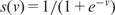is called the ‘activation function’. The unknown parameters 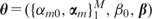are estimated by minimizing the sum of squared errors, 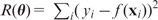, via the gradient descent method (i.e. moving along the direction with the steepest descent), also called back-propagation in this setting. In order to avoid overfitting, a penalty is often added to the loss function: , where is the sum of squares of all the parameters. This modified loss function is what we use in this work for training neural networks. Here, λ is referred to as the weight decay.

SVM

Suppose each data point in consideration belongs to one of the two classes, the SVM aims to find a boundary in the p-dimensional space that not only separates the two classes of data points but also maximizes its margin of separation. The method can also be adapted to deal with regression problems, in which case the prediction function is represented by

6

where K is a chosen kernel function (e.g. polynomial or radial kernels). The problem of deciding the optimal boundary is equivalent to minimizing

where V(ċ) is an ‘ε-insensitive’ error measure and C is a positive constant that can be viewed as a penalty to overly complex boundaries (40). The computation of SVM is carried out by convex quadratic programming. The training data whose in the solution (6) are called support vectors.

Additive models: MARS, boosting and BART

Another large class of learning methods, based on additive models, approximates f(X) by a summation of many nonlinear basis functions, i.e.

where g_m(X;γ_m) is a basis function with parameter γ_m. Different forms of basis functions with different ways to select and estimate them give rise to various learning methods, including MARS (32), boosting (34) and BART (35) among others. In some sense, neural networks and SVM can also be formulated as additive models. In MARS, the collection of basis functions is

where ‘’ means positive part: if x > 0 and otherwise. These basis functions are called linear splines. The g_m(X;γ_m) in MARS can be a function in or a product of up to d such functions. The learning of MARS is performed by forward addition and background deletion of basis functions to minimize a penalized least square loss, which incurs a penalty of λ per additional degree of freedom of the model. Consequently, λ and d determine the model complexity of MARS.

Regression trees are widely used as basic functions for boosting and BART. Let T denote a regression tree with a set of interior and terminal nodes. Each interior node is associated with a binary decision rule based on one feature, typically of the form {X_j ≤ a} or {X_j > a} for 1 ≤ j ≤ p. Suppose the number of terminal nodes is B. Then the tree partitions the feature space into B disjoint regions, each associated with a parameter 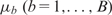(Figure 1A). Accordingly, the tree with its associated parameters represents a piece-wise constant function with B distinct pieces (Figure 1B). We denote this function by , where . Then, the additive regression tree model approximates f (X) by the sum of M such regression trees:

7

in which each tree T_m is associated with a parameter vector . The number of trees M controls the model complexity, and it is usually large (100–200), which makes the model flexible enough to approximate the underlying relationship between Y and X.

Figure 1.

A regression tree with two interior and three terminal nodes. (A) The decision rules partition the feature space into three disjoint regions: {X₁ ≤ c,X₂ ≤ d},{X₁ ≤ c,X₂ > d} and {X₁ > c}. The mean parameters attached to these regions are ]. (B) The piece-wise constant function defined by the regression tree with c = 3, d = 2 and .

In the original AdaBoost algorithm (34), an additive model is produced via iteratively re-weighting the training data according to the training error of the current classifier. Later, a more general framework was developed to formulate boosting algorithms as a method of function gradient descent (41), which is what we use in this work. For a gradient boosting machine under square loss, given a current additive model a regression tree is fitted to the current residuals and then the additive model is updated to

where 0 < ν ≤ 1 is the shrinkage parameter (learning rate). Applying this recursion for M iterations gives the boosting additive tree model as in Equation (7).

BART completes Bayesian inference on model (7) with prescribed prior distributions for both the tree structure and the associated parameters, and the variance σ² of Gaussian noise ε (2). The prior distribution for the tree structure is specified conservatively so that the size of each tree is kept small, which forces it to be a weak learner. The priors on and σ² also contribute to alleviating overfitting. A Markov chain Monte Carlo method (BART MCMC) was developed (35) for sampling from the posterior distribution , in which both the tree structures and the parameters are updated simultaneously. Given a new feature vector x*, BART predicts the response y* by the average response of all sampled additive trees instead of using only the best model. In this sense, BART has the nature of Bayesian model averaging.

RESULTS

We applied the predictive modeling approach outlined above to recently published ChIP-chip data sets of the TFs Oct4 and Sox2 in human embryonic stem cells (ESC) (42), with a comparative study on various mentioned learning methods using 10-fold cross-validations (CVs). We discovered consistently a Sox–Oct composite motif from both the Oct4 and the Sox2 ChIP-chip data sets using a de novo motif search algorithm. This motif is known to be recognized by the protein complex of Oct4 and Sox2, the target TFs in the ChIP-chip experiments, and thus we included it in our precompiled motif set. In addition, we extracted 223 motifs from TRANSFAC release 9.0 (43) and literature survey to compile a final list of 224 PWMs. Please see Supplementary Text for the details. The sequence sets, ChIP-enrichment values and feature matrices are available at http://www.stat.ucla.edu/~zhou/ChIPLearn/. We also conducted a simulation study to further verify the performances of the methods.

The Oct4 ChIP-chip data in human ESCs

Boyer et al. (42) reported 603 Oct4-ChIP-enriched regions (positives) in human ESCs with DNA microarrays covering −8 kb to +2 kb of ∼17 000 annotated human genes. We randomly selected another 603 regions with the same length distribution from the genomic regions targeted by the DNA microarrays (negatives), i.e. kb of the annotated genes. The ChIP-intensity measure defined as the average array-intensity ratio of ChIP samples over control samples was attached to each of the 1206 ChIP-regions. We treated the logarithm of the ChIP-intensity measure as the response variable Y and the features extracted from the genomic sequences as the explanatory variables X. This produced a data set of 1206 observations with 269 features (224 PWMs, 3 genetic features, 10 dimers, 32 trimers: see Equation 3), called the Oct4 data set henceforth.

CVs. We compared the following statistical learning algorithms via a 10-fold CV procedure on the Oct4 data set: (i) LR-SO/LR-Full, linear regression using the Sox–Oct composite motif only or using all the 269 features; (ii) Step-SO/Step-Full, stepwise linear regression starting from LR-SO or starting from LR-Full; (iii) NN-SO/NN-Full, neural networks with the Sox–Oct composite motif feature or all the features as input; (iv) Step+NN, neural networks with the features selected by Step-SO as input; (v) MARS using all the features; (vi) SVM for regression with various kernels; (vii) Boost, boosting with regression trees as base learners and (viii) BART with different number of trees.

The observations were divided randomly into 10 subgroups of equal size. Each subgroup (called ‘the test sample’) was left out in turn and the remaining nine subgroups (called ‘the training sample’) were used to train a model using one of the above methods. Then the observed responses of the test sample were compared to those predicted by the trained model. We used the correlation coefficient between the predicted and the observed responses as a measure of the predictive power of a tested method. This measure is invariant under linear transformation, and can be understood as the fraction of variation in the response variable attributable to the explanatory features. We call this measure the CV-correlation (CV-cor) henceforth. Treating the LR-SO method as the baseline for our comparison, which only involves the single target motif, we are interested in testing whether other genomic sequence features can significantly influence the prediction of the ChIP enrichment, which can be viewed as a surrogate of the TF–DNA binding affinity. The predictive modeling approach employed here facilitates us a coherent framework to identify useful features, which may lead to testable hypotheses that enhance our understanding of the protein–DNA interaction.

As reviewed in the Materials and methods section and listed in Table 1, sophisticated learning methods have their respective tuning parameters. We conducted CVs for a wide range of these tuning parameters and identified the optimal value in terms of CV-cor. A proper common practice in the field is to further divide the samples to tune these parameters. But, here we chose not to do so since we were also interested in comparing the robustness of different methods with different tuning parameters. The detailed description and results of the CVs, including the way we chose the tuning parameters, are given in the Supplementary Text.

Table 1.

Ten-fold CVs of the Oct4 ChIP-chip data

Method	Tuning parameters	CV-cor	SD
LR-SO	–	0.446 (0%)	0.044
LR-Full	–	0.491 (10%)	0.064
Step-SO	–	0.535 (20%)	0.045
Step-Full	–	0.513 (15%)	0.054
NN-SO	# of nodes, weight decay	0.468 (5%)	0.063
Step+NN	# of nodes, weight decay	0.463 (4%)	0.067
MARS	Interaction d, penalty λ	0.580 (30%)	0.043
SVM	Cost C	0.547 (23%)	0.054
Boost	# of trees M	0.581 (30%)	0.048
BART	# of trees M	0.600 (35%)	0.044

Reported here are the average CV-cors. The percentage in the parentheses is calculated by the percent of improvement over the CV-cor of LR-SO. SD is the standard deviation across 10 test samples. The detailed definitions of tuning parameters are reviewed in the MATERIALS AND METHODS section and further discussed in Supplementary Text.

The overall comparison results are briefly summarized in Table 1. The average CV-cor (over 10 test samples) of LR-SO was 0.446. Among all the linear regression methods, Step-SO achieved the highest CV-cor of 0.535. NN-SO and Step+NN showed a slight improvement over LR-SO after tuning weight decay and the number of hidden nodes, while the performance of NN-Full (optimal CV-cor <0.38) was unsatisfactory. SVM showed 23% improvement over LR-SO and it was quite robust with stable CV-cors for C ≥ 1. The optimal results of MARS, boosting and BART were all substantially superior to the other methods. However, they had different degrees of robustness to their respective tuning parameters. The CV-cor of MARS could drop below 0.46 if one did not choose a good value for its penalty cost λ, while the other two methods were much more robust. For example, the CV-cors of BART with all the tested numbers of trees (M) ranging from 20 to 200 varied only between 0.592 and 0.6, which uniformly outperformed the optimal tuned results of all the other methods. This suggests that in practice the users may not need to worry too much about the tuning parameters in BART and boosting, but apply these methods with the default settings comfortably to their data sets. This is a significant advantage over some other learning methods such as NN and MARS. The SD in CV-cor across the 10 test samples for all the methods were quite comparable (around 0.04–0.05) except that the LR-Full and NN methods showed larger variability.

A common method for predicting whether a particular DNA sequence can be bound by a TF is to score the sequence by the PWM of the TF. This is equivalent to using LR-SO for the binding prediction. Thus, our study demonstrated that sophisticated statistical learning tools such as MARS, SVMs, boosting and BART can all significantly improve the basic LR-SO prediction by including more sequence features.

Sequence features selected by BART

We chose BART with 100 trees to perform a detailed study on the full data set (with 1206 observations). The posterior mean tree size (of a base learner) measured by the number of terminal nodes was 2.31. Thus, each tree in the model was indeed quite simple. We define the posterior inclusion probability P_in of a feature by the fraction of sampling iterations in which the feature is included in the additive trees. Figure 2 shows the P_in's for all the 269 features in descending order, and 22 of them are >0.5 (Table 2). In addition, the average number of times a feature is used in each posterior sample of the BART model (a feature can be used a number of times by a BART model since the model is an aggregation of many regression trees), called the per-sample inclusion (PSI), is also reported in the table as another measure of the importance of the feature.

Figure 2.

The posterior inclusion probability P_in of all the features in descending order in the BART model for the Oct4 data set.

Table 2.

The top 22 features in the BART model for the Oct4 ChIP-chip data

Feature	Pin	PSI	t	Notes/Consensus
SoxOcta	1.000	3.50	14.0	CWTTNWTATGYAAAT
GC	1.000	1.56	2.7	Background
CAA	0.998	2.18	4.4	Background
CCA	0.987	1.45	−5.2	Background
Length	0.964	1.37	7.8	Sequence length
HSF1_Q6	0.963	1.32	1.2	TTCTRGAAVNTTCTYM
AA	0.945	1.41	2.7	Background
G/C	0.870	1.46	0.9	GC content
UF1H3b_Q6a	0.821	1.14	7.8	GCCCCWCCCCRCC
CA	0.760	1.19	−6.1	Background
CGC	0.723	1.04	4.6	Background
AAT	0.693	0.96	0.7	Background
cs	0.691	0.91	8.0	Conservation
OCT_Q6a	0.649	0.95	10.2	TNATTTGCATN
NFY_Q6a	0.628	0.84	2.8	TRRCCAATSRN
CGA	0.622	0.87	7.7	Background
OCT1_Q6a	0.589	0.79	8.8	ATGCAAATNA
OCT1_Q5_01a	0.575	0.78	10.2	TNATTTGCATW
GA	0.564	0.78	−0.5	Background
E2F_Q3_01	0.540	0.75	8.6	TTTSGCGSG
GCA	0.528	0.70	2.5	Background
E2F1_Q4_01	0.512	0.68	8.8	TTTSGCGSG

The ‘t’ is the t-statistics between the positive and negative ChIP regions. ^aMotifs with reported functions in ESCs.

The top feature under both the overall and the PSI statistics is the Sox–Oct composite motif, consistent with the existing biological knowledge that Sox2 is one of the most important co-regulators of Oct4 and they form a protein complex to bind to the composite sites. Besides, we found another eight motifs with P_in > 0.5, among which OCT_Q6, OCT1_Q6 and OCT1_Q5_01 represent all the variants of the Oct4 motif in our compiled list. This implies the high sensitivity of our method in detecting functional motifs. The remaining five motifs, Hsf1, Uf1h3b, Nfy_Q6, E2F and E2F1, may be co-regulators of Oct4 or other functional TFs in ESCs. As reported recently (44), the TF Nfyb regulates ES proliferation in both mouse and human ESCs by binding specifically to the motif Nfy_Q6 in the promoter regions of ES-upregulated genes. Nfyb were also reported to co-activate genes with E2F via adjacent binding sites (45). The significant roles of both motifs in our model suggest that their co-activation of genes in ESCs may be recruited or enhanced by Oct4 binding. The motif Uf1h3b contains the consensus of the Klf4 motif (CCCCRCCC) (46). The TF Klf4, together with Oct4, Sox2 and c_Myc, can reprogram highly differentiated somatic cells back to pluripotent ES-like cells (47). In a reported Oct4 enhancer (48) there is a highly conserved site that matches the consensus of the Uf1h3b motif within 40 bp of a known Sox–Oct site. These external data confirmed the biological relevance in ESCs of at least six out of the nine motifs identified by the BART model (indicated in Table 2). It is interesting to note that the Hsf1 motif is not highly enriched in the positive ChIP regions (with small t-statistic), yet it has a very high P_in, indicating that it may interact with other factors in a nonlinear way. The sequence length was selected in the model as well, which served to balance out the potential bias in ChIP-intensity caused by the length difference of repeat elements in the original sequences.

A surprising yet interesting finding is the high inclusion probabilities of many nonmotif features, such as ‘GC’, ‘CAA’, ‘CCA’, ‘AA’ and ‘G/C’. This is also true for the learning results of other methods, such as stepwise linear regression and boosting, especially among the features with significant roles in these models (Figure 3). It is possible that some of these words are directly responsible for the interaction strength between Oct4 and its DNA-target region, such as ‘CAA’ and ‘AA’, which occur in the Oct4 motif consensus (ATGCAAAT). They may also contribute to the bending of the DNA sequences and thereby promote the assembly of elaborate protein–DNA interacting structures (49). To further verify their effect in predictive modeling, we excluded nonmotif features from the input, and applied BART (with 100 trees), MARS (), MARS () and Step-SO to the resulting data set to perform 10-fold CVs. The parameters for MARS were chosen based on the CV results in Table 1 (also see Supplementary Text). The CV-cors turned out to be 0.510, 0.511, 0.478 and 0.456 for the above four models, respectively, which decreased substantially (about 12–15%) compared to the CV-cors of the corresponding methods with all the features.

Figure 3.

The histograms of the non-motif features (dark bars) and all the features (light bars) selected in (A) Step-SO and (B) boosting with 100 trees on the Oct4 data set. In Step-SO, selected features are classified into categories by regression P-values. In boosting, they are classified by their relative influence normalized to sum up to 100%.

Using this data set, we also compared the use of heterogeneous and homogeneous Markov background models for motif feature extraction. The heterogeneous background model is discussed in the Feature extraction section and is used for computing motif features in the above analysis. For the homogeneous background model, we used all the nucleotides in a sequence to build a first-order Markov chain. With these two different background models, we calculated motif scores for all the Oct4-family matrices in the 224 PWMs, i.e. the Sox–Oct composite motif, OCT1_Q6, OCT_Q6 and OCT1_Q5_01. We observed that, for all the four matrices, the motif scores under the heterogeneous background model showed higher correlations with the log-ChIP intensity than the scores under the homogeneous background model (Supplementary Table 1). We further computed the t-statistic for each motif score between the positive and negative ChIP-regions. Similarly, using the heterogeneous background model enhanced the separation between the positive and negative regions by resulting in larger t-statistics (Supplementary Table 1).

Prediction and validation in mouse data

The trained predictive models are useful computational tools to predict whether a piece of DNA sequence can be bound by the TF. They can be utilized to identify novel binding regions outside of the microarray coverage or not detected (false negatives) by the ChIP-chip experiment, and also to predict binding regions in other closely related species. As a proof of the concept, we applied the trained Oct4 BART and boosting models in the above human data to discriminate ∼1000 Oct4-bound regions in mouse ESCs (50) from 2000 random upstream sequences with the identical length distribution. After extracting the same 269 features, we predicted ChIP-binding intensities of the 3000 sequences by the BART and boosting models, respectively. As a comparison, we also scanned each sequence to compute its average matching score to the Sox–Oct composite motif found by de novo search (called scanning method) for measuring the likelihood to be bound by the TF as suggested by many other studies (29). By gradually decreasing the threshold value, we obtained both higher sensitivity and more false positive counts for each method. We focused on the part where all the three methods predicted < 500 random sequences as being bound by Oct4. As reported in Figure 4, both the BART and boosting models significantly reduced the number of false positives (random sequences) for almost all the sensitivity levels compared to the scanning method, which corresponded to an average of ∼30% decrease in the false positive rate. Note that the Oct4 target genes identified by the ChIP-based assays are substantially different (with < 10% of overlapping targets) between human and mouse (50). Thus, our result here represents an unbiased validation of the computational predictions. It also suggests that the binding pattern of Oct4 as characterized by our predictive models is very similar between the two species, even though its target genes may be quite different.

Figure 4.

Sensitivity and false positive counts for the BART, boosting and Sox-Oct scan methods in discriminating Oct4-bound sequences in mouse ESCs and random upstream sequences.

The Sox2 ChIP-chip data in human ESCs

We next applied our method to the 1165 Sox2 positive-ChIP regions identified by (42), accompanied by the same number of randomly selected regions from [] kb of a gene with the same length distribution. Although known to co-regulate genes in the undifferentiated state, the target genes of Sox2 and Oct4 identified by ChIP-based experiments are substantially different (42). Besides testing our method, we are also interested in comparing the sequence features of the binding regions of these two regulators.

We extracted the same 269 features as in the previous subsection for each sequence in this Sox2 data set, and conducted 10-fold CVs to study the performances of the aforementioned statistical learning methods (more details in Supplementary Text). As shown in Table 3, BART with different tree numbers (CV-cors between 0.561 and 0.572) again outperformed all the other methods with optimal parameters, while boosting and MARS showed slightly worse but comparable performances. The improvement of these three methods over LR-SO, the baseline performance, was >  54%. It is important to note that BART again performed very robustly while many other methods, such as NN, MARS and SVM, showed more variable performances with different choices of their tuning parameters (Supplementary Text). In addition, the SD in CV-cor for BART was the smallest among all the methods. We further applied Step-SO, MARS () and BART (M = 100), with only motif features as input, and obtained CV-cors of 0.465, 0.469 and 0.500, respectively. One sees that all of them performed significantly worse than the corresponding methods using all the features. This confirms our hypothesis that nonmotif features are essential components of the underlying model for TF–DNA binding.

Table 3.

Ten-fold CV results of the Sox2 data set

Method	CV-cor	SD	Method	CV-cor	SD
LR-SO	0.358 (0%)	0.049	LR-Full	0.494 (38%)	0.044
Step-SO	0.513 (43%)	0.043	Step-Full	0.509 (42%)	0.046
NN-SO	0.364 (2%)	0.053	Step+NN	0.465 (30%)	0.047
MARS	0.553 (54%)	0.050	SVM	0.526 (47%)	0.044
Boost	0.560 (56%)	0.047	BART	0.572 (60%)	0.038

The same notations and definitions of tuning parameters are used as in Table 1.

We re-applied BART with 100 trees to the full Sox2 data set with 2330 observations. There are 29 features with P_in > 0.5, including three generic features, 10 background frequencies and 16 motifs (Supplementary Table 2). As indicated in the Table, 7 out of the top 9 motifs were reported to be recognized by functional TFs in ESCs or differentiation. In agreement with the fact that the target TF is Sox2, the top three features include the Sox–Oct composite and the Sox2 motifs. Other potential motifs identified by BART that co-occur with Sox2 binding include Nanog (), Nkx2.5 (0.70), Uf1h3b (0.67), P53 (0.64) and Gata-binding proteins (0.59). Among them, Nanog is known as a crucial TF that co-regulates with Sox2 and Oct4, and P53 is a marker gene in ESCs (51,52). Interestingly, the Sox2 motif is overwhelmingly overrepresented (p = 2 × 10⁻¹²) in the Nanog-bound regions of up-regulated genes in mouse ESCs (53). These analyses strongly support the tight regulatory interaction between Sox2 and Nanog in both human and mouse embryonic development. Nkx2.5 and Gata4 are known cooperative TFs in endoderm differentiation (54). Both of them are suppressed in ESCs but highly expressed once the cells start to differentiate into early endoderm. These results suggest a hypothesis for further investigation that genes repressed by Sox2 in ESCs may be activated later for endoderm development once Gata4 and Nkx2.5 are expressed and bind to their motifs in the Sox2 bound regions (Figure 5). Such competitive binding of Gata/Nkx2-families could be an efficient mechanism to accelerate the termination of Sox2-bound repression when differentiation is initiated.

Figure 5.

A hypothesis of competitive binding between Sox2 and Gata4/Nkx2.5. In undifferentiated ES cells, Sox2 binds to a regulatory sequence (bracket region) to repress a target gene, while Gata4 and Nkx2.5 are not expressed. Later upon differentiation, Gata4 and Nkx2.5, both highly expressed, out-compete Sox2 to bind to the same region, thus terminating the repression of the downstream gene.

Furthermore, we compared the BART models inferred from the Oct4 and the Sox2 data sets, and found that BART identified 22 and 29 features with P_in > 0.5, respectively. Among them, 10 features are in common, which is much higher than that expected by chance with a P-value of 1 × 10⁻⁵ and a 4.2-fold enrichment. This is consistent with the known co-regulation of Oct4 and Sox2 in ES cells. A notable common motif feature with high P_in in both models is the Uf1h3b motif, which contains the consensus of Klf4 whose motif has not been included in TRANSFAC yet. This result predicted Klf4 as a common co-regulator of Oct4 and Sox2 in ESCs. The ChIP-chip data of Plath and colleagues (Sridharan et al., manuscript in preparation) provided an experimental validation of this prediction, in which the respective target genes of Oct4, Sox2, Klf4 and other important ESC regulators were identified. Among the ∼1400 Klf4 target genes, 500 and 535 of them were also bound by Oct4 and Sox2, respectively. Furthermore, the actual binding regions shared at least 650 bp for >75% of the common targets. These experimental data confirmed the co-regulation between Klf4 and the other two master TFs. On the other hand, sequence features specific to each data set provide a basis to distinguish the binding patterns of Oct4 and Sox2. For example, Nfy was only identified with high P_in in the Oct4 data set, whereas Nanog only co-occurred in the Sox2 bound regions. The missing of Nanog in the Oct4 BART model is consistent with an independent observation that the Nanog motif is not enriched in the Oct4-bound enhancers in mouse ESCs (53), although significant overlaps in target genes of these two TFs were reported (42,50). One possible explanation, which awaits future experimental investigations, is that the direct DNA binding of Nanog may depend on its interactive TFs. In the presence of Oct4, Nanog may not bind to DNA directly but co-regulate genes with Oct4 via protein–protein interactions (55).

A simulation study

We performed a simulation study as a final test on the effectiveness of the predictive modeling approach, which allows us to evaluate its accuracy in identifying true sequence features, especially motifs that determine the observed measurements. We generated 1000 sequences, each from a first-order Markov chain, of length uniformly distributed between 800 and 1200. For each of the first 500 sequences, we inserted one, two or three Oct4 motif sites with probability 0.25, 0.5 or 0.25, respectively. Furthermore, we inserted one site for each of the three motifs, Sox2, Nanog and Nkx2.5, independently with probability 0.5. We calculated the score of an inserted site by Equation (4). For each motif we obtained the sum of the site scores for a sequence, denoted by Z₁, …,Z₄ for Oct4, Sox2, Nanog and Nkx2.5, respectively. Then, we defined the motif score for a sequence by for . Denote by X₅ the GC content of a sequence. We normalized these five features by their respective standard deviations so that the rescaled features have a unit variance. Then, the observed ChIP-intensity Y for a sequence was simulated as:

8

where . This model states that X₁ is the primary TF with three interactive factors (X₂,X₃,X₄) and the GC content (X₅) has a positive effect on the ChIP-intensity. The signal-to-noise-ratio (SNR) of a simulated data set is defined as Var( f(X))/σ² ≡ Var(Y )/σ² − 1, which is the ratio of the variance of the true ChIP-intensity f(X) over the noise variance σ². We simulated 10 independent sequence sets, and then generated observed ChIP-intensities according to (8) with , 1/1 and 1/2, respectively.

We applied the same sequence feature extraction as in the previous sections to the simulated data sets and compared the performances of stepwise regression, MARS, boosting and BART in terms of their response prediction and error rates of sequence feature selection. We calculated the correlation between a predicted response and the true ChIP-intensity f(X), denoted by . Then the expected correlation between the predicted and a future observed response , called the expected predictive correlation (EP-cor), was computed by

where is independent of and f(X). We applied MARS (), boosting and BART with 100 trees here given that these were their optimal tuning parameters in the Oct4 data set, which is roughly of the same size as the simulated data. The comparison of the results of these methods is given in Table 4.

Table 4.

Performance comparison on the simulated data sets

Method	SNR	1/0.6	1/1	1/2
	EP-cor	0.579 (0.009)	0.497 (0.012)	0.368 (0.010)
Step-LR	NT	3.8 (0.42)	3.8 (0.42)	3.3 (0.67)
	NF	4.9 (2.64)	8.6 (3.63)	7.5 (3.54)
	EP-cor	0.579 (0.011)	0.498 (0.013)	0.376 (0.018)
MARS	NT	3.9 (0.32)	3.5 (0.53)	3.3 (0.48)
	NF	4.4 (1.78)	4.2 (1.81)	4.6 (2.80)
	EP-cor	0.603 (0.007)	0.528 (0.010)	0.405 (0.011)
Boost	NT	3.9 (0.32)	3.7 (0.48)	3.5 (0.53)
	NF	0.6 (0.70)	2.4 (1.58)	5.9 (1.85)
	EP-cor	0.636 (0.009)	0.551 (0.007)	0.416 (0.006)
BART	NT	4.0 (0.00)	3.6 (0.70)	3.5 (0.71)
	NF	1.8 (1.40)	2.5 (1.18)	2.5 (1.43)

Reported are the averages (standard deviations in the parentheses) over 10 independent data sets. N_T and N_F are the numbers of true and false motifs identified, respectively.

As expected, with the increase of the noise level, the average EP-cor and the accuracy of motif identification decreased for all the tested methods. Consistent with the other two data sets, the EP-cors of BART were the highest at all the levels of SNR. When we set the threshold of P_in to 0.7, BART identified on average >85% of the true motifs accompanied by at most 2.5 false positives. For stepwise linear regression (Step-LR), only features with a regression P-value <0.01 were used for computing error rates in motif identification since including all the covariates selected by the method resulted in an overly large number of false positives. At comparable sensitivity levels (N_T), BART reported significantly fewer false positives (N_F) for all the SNR levels than Step-LR and MARS (Table 4). The relative influence of a feature selected by boosting was measured by the reduction of squared error attributable to the feature. We ranked all the selected features by their relative influence and set a reasonable threshold to obtain similar sensitivity levels as those of BART. We noticed that these two methods showed comparable error rates in motif identification for SNR ≥ 1, but the boosting method seemed to result in a higher false positive rate at the lowest SNR level (=1/2).

DISCUSSION

We have demonstrated in this article how predictive modeling approaches can reveal subtle sequence signals that may influence TF–DNA binding and generate testable hypotheses. Compared with some other more system-based approaches to gene regulation, such as building a large system of differential equations or inferring a complete Bayesian network, predictive modeling is more intuitive, more theoretically solid (as many in-depth statistical learning theories have been developed), more easily validated (by CV), and can generate more straightforward testable hypotheses.

Our main goal here is to conduct a comparative study on the effectiveness of several statistical learning tools for combining ChIP-chip/expression and genomic sequence data to tackle the protein–DNA binding problem. Because of the generality of these tools, we are able to include sequence features besides TF motifs, such as background words, GC content, and a measure of cross-species conservation. The finding that these nonmotif features can significantly improve the predictive power of all the tested methods indicates a potentially important yet less understood role these sequence features play in TF–DNA interactions. They may help the localization of a TF on the DNA for precise recognition of its binding sites, or may have a function with chromatin associated factors and histone modification activities. It is generally believed that many other factors in addition to the sequence specificity of short TFBSs contribute to TF–DNA binding. Along this direction, we have proposed a general framework to explore and characterize potentially influential factors.

In both ChIP-chip data sets, we not only unambiguously identified all the binding motifs for the target TFs, Oct4 and Sox2, but also discovered a number of verified cooperative or functional regulators in ESCs, such as Nanog, Klf4, Nfyb and P53. As a principled way to utilize both positive (i.e. binding sequences) and negative (nonbinding) information, the predictive modeling approach provides a powerful alternative for detecting TF-binding motifs to those more popular generative model-based tools (3–6). Noting that the stepwise linear regression methods (Step-Full, Step-SO, and Step-LR) are equivalent to MotifRegressor (29) and MARS is equivalent to MARSMotif (30) with all the known and discovered (Sox–Oct) motifs as input, we have shown that BART and boosting using all three categories of sequence features outperformed MotifRegressor and MARSMotif significantly in all of our examples.

For a generative modeling approach, separate statistical models are fitted to TF-bound (positive) and background (negative) sequences, and then discriminant analysis based on posterior odds ratio or likelihood ratio is applied to construct prediction rules. In contrast, a predictive modeling approach targets at prediction by modeling directly the condition distribution of TF-binding given extensively extracted sequence features. As shown in this article by both real and simulated data sets, modern statistical learning tools such as boosting and BART have made it possible to estimate this conditional distribution quite accurately for the TF-binding problem. These two approaches have their own respective advantages. If the underlying data generation process is unclear or difficult to model, predictive approaches have the advantage to construct a nonparametric conditional distribution from the training data. On the other hand, generative models are usually built with more explicit assumptions that help us understand the underlying science and can capture key characteristics of a biological or physical system. Typical examples of generative models in gene-regulation problems include, for example, the mixture modeling of DNA sequence motifs (2) and the graphical model for protein–DNA interaction measured with ChIP-chip data (56).

Finally, our study suggests that the Bayesian learning method BART is a good tool for analyzing high-dimensional genomic data because of its high predictive power, its explicit quantification of uncertainty, and its interpretability. First, like boosting, BART is an ensemble learning method, which approximates an unknown relationship by an aggregation of a large number of simple models (small trees). Second, the Bayesian formulation of BART leads to not only the ‘optimal’ model, but also a posterior distribution on the space of all possible models, which can be used to predict the response of a new observation by weighted averaging predictions from all models. This model averaging approach tends to improve the model's; predictive power in general. Third, the variable selection procedure is a coherently built-in feature of BART and performs quite well in identifying important and relevant sequence features that contribute to TF–DNA interactions in all the examples. With the rapid accumulation of large-scale genomic data, we believe that flexible statistical learning methods such as BART and boosting will be very useful for studying a large class of biological problems including cis-regulatory analysis.

SUPPLEMENTARY DATA

Supplementary Data are available at NAR Online.

REFERENCES

- 1.Stormo GD, Hartzell GW. Identifying protein-binding sites from unaligned DNA fragments. Proc. Natl Acad. Sci. USA. 1989;86:1183–1187. doi: 10.1073/pnas.86.4.1183. [DOI] [PMC free article] [PubMed] [Google Scholar]
- 2.Lawrence CE, Altschul SF, Boguski MS, Liu JS, Neuwald AF, Wooton JC. Detecting subtle sequence signals: a Gibbs sampling strategy for multiple alignment. Science. 1993;262:208–214. doi: 10.1126/science.8211139. [DOI] [PubMed] [Google Scholar]
- 3.Bailey TL, Elkan C. Fitting a mixture model by expectation maximization to discover motifs in biopolymers. Proc. Int. Conf. Intell. Syst. Mol. Biol. 1994;2:28–36. [PubMed] [Google Scholar]
- 4.Liu X, Brutlag DL, Liu JS. BioProspector: discovering conserved DNA motifs in upstream regulatory regions of co-expressed genes. Pac. Symp. Biocomput. 2001;6:127–138. [PubMed] [Google Scholar]
- 5.Roth FR, Hughes JD, Estep PE, Church GM. Finding DNA regulatory motifs within unaligned noncoding sequences clustered by whole genome mRNA quantization. Nat. Biotechnol. 1998;16:939–945. doi: 10.1038/nbt1098-939. [DOI] [PubMed] [Google Scholar]
- 6.Liu XS, Brutlag DL, Liu JS. An algorithm for finding protein-DNA binding sites with applications to chromatin immunoprecipitation microarray experiments. Nat. Biotechnol. 2002;20:835–839. doi: 10.1038/nbt717. [DOI] [PubMed] [Google Scholar]
- 7.Jensen ST, Liu XS, Zhou Q, Liu JS. Computational discovery of gene regulation binding motifs: a Bayesian perspective. Stat. Sci. 2004;19:188–204. [Google Scholar]
- 8.Elnitski L, Jin VX, Farnham PJ, Jones SJM. Locating mammalian transcription factor binding sites: a survey of computational and experimental techniques. Genome Res. 2006;16:1455–1464. doi: 10.1101/gr.4140006. [DOI] [PubMed] [Google Scholar]
- 9.Benos PV, Lapedes AS, Stormo GD. Probabilistic code for DNA recognition by proteins of the EGR family. J. Mol. Biol. 2002;323:701–727. doi: 10.1016/s0022-2836(02)00917-8. [DOI] [PubMed] [Google Scholar]
- 10.Bulyk ML, Johnson PLF, Church GM. Nucleotides of transcription factor binding sites exert interdependent effects on the binding affinities of transcription factors. Nucleic Acids Res. 2002;30:1255–1261. doi: 10.1093/nar/30.5.1255. [DOI] [PMC free article] [PubMed] [Google Scholar]
- 11.Barash Y, Elidan G, Friedman N, Kaplan T. Modeling dependence in protein-DNA binding sites. Proc. Int. Conf. Res. Comp. Mol. Biol. 2003;7:28–37. [Google Scholar]
- 12.Zhou Q, Liu JS. Modeling within-motif dependence for transcription factor binding site predictions. Bioinformatics. 2004;20:909–916. doi: 10.1093/bioinformatics/bth006. [DOI] [PubMed] [Google Scholar]
- 13.Zhao Y, Huang XH, Speed TP. Finding short DNA motifs using permuted Markov models. J. Comput. Biol. 2005;12:894–906. doi: 10.1089/cmb.2005.12.894. [DOI] [PubMed] [Google Scholar]
- 14.Workman CT, Stormo GD. ANN-Spec: a method for discovering transcription factor binding sites with improved specificity. Pac. Symp. Biocomput. 2000;5:467–478. doi: 10.1142/9789814447331_0044. [DOI] [PubMed] [Google Scholar]
- 15.Smith AD, Sumazin P, Zhang MQ. Identifying tissue-selective transcription factor binding sites in vertebrate promoters. Proc. Natl Acad. Sci. USA. 2005;102:1560–1565. doi: 10.1073/pnas.0406123102. [DOI] [PMC free article] [PubMed] [Google Scholar]
- 16.Hong P, Liu XS, Zhou Q, Lu X, Liu JS, Wong WH. A boosting approach for motif modeling using ChIP-chip data. Bioinformatics. 2005;21:2636–2643. doi: 10.1093/bioinformatics/bti402. [DOI] [PubMed] [Google Scholar]
- 17.Wasserman WW, Fickett JW. Identification of regulatory regions which confer muscle-specific gene expression. J. Mol. Biol. 1998;278:167–181. doi: 10.1006/jmbi.1998.1700. [DOI] [PubMed] [Google Scholar]
- 18.Frith MC, Hansen U, Weng Z. Detection of cis-element clusters in higher eukaryotic DNA. Bioinformatics. 2001;17:878–889. doi: 10.1093/bioinformatics/17.10.878. [DOI] [PubMed] [Google Scholar]
- 19.Xing EP, Wu W, Jordan MI, Karp RM. Comput. Syst. Bioinformatics Conference 2003. Stanford, CA: 2003. LOGOS: a modular Bayesian model for de novo motif detection. [PubMed] [Google Scholar]
- 20.Zhou Q, Wong WH. CisModule: de novo discovery of cis-regulatory modules by hierarchical mixture modeling. Proc. Natl Acad. Sci. USA. 2004;101:12114–12119. doi: 10.1073/pnas.0402858101. [DOI] [PMC free article] [PubMed] [Google Scholar]
- 21.Thompson W, Palumbo MJ, Wasserman WW, Liu JS, Lawrence CE. Decoding human regulatory circuits. Genome Res. 2004;14:1967–1974. doi: 10.1101/gr.2589004. [DOI] [PMC free article] [PubMed] [Google Scholar]
- 22.Gupta M, Liu JS. De novo cis-regulatory module elicitation for eukaryotic genomes. Proc. Natl Acad. Sci. USA. 2005;102:7079–7084. doi: 10.1073/pnas.0408743102. [DOI] [PMC free article] [PubMed] [Google Scholar]
- 23.Zhou Q, Wong WH. Coupling hidden Markov models for the discovery of cis-regulatory modules in multiple species. Ann. Appl. Stat. 2007;1:36–65. [Google Scholar]
- 24.Berg OG, von Hippel PH. Selection of DNA binding sites by regulatory proteins: statistical-mechanical theory and application to operators and promoters. J. Mol. Biol. 1987;193:723–750. doi: 10.1016/0022-2836(87)90354-8. [DOI] [PubMed] [Google Scholar]
- 25.Stormo GD, Fields DS. Specificity, free energy and information content in protein-DNA interactions. Trends Biochem. Sci. 1998;23:109–113. doi: 10.1016/s0968-0004(98)01187-6. [DOI] [PubMed] [Google Scholar]
- 26.Liu JS, Neuwald AF, Lawrence CE. Bayesian models for multiple local sequence alignment and Gibbs sampling strategies. J. Am. Stat. Assoc. 1995;90:1156–1170. [Google Scholar]
- 27.Bussemaker HJ, Li H, Siggia ED. Regulatory element detection using correlation with expression. Nat. Genet. 2001;27:167–171. doi: 10.1038/84792. [DOI] [PubMed] [Google Scholar]
- 28.Keles S, van der Laan M, Eisen MB. Identification of regulatory elements using a feature selection method. Bioinformatics. 2002;18:1167–1175. doi: 10.1093/bioinformatics/18.9.1167. [DOI] [PubMed] [Google Scholar]
- 29.Conlon EM, Liu XS, Lieb JD, Liu JS. Integrating regulatory motif discovery and genome-wide expression analysis. Proc. Natl Acad. Sci. USA. 2003;100:3339–3344. doi: 10.1073/pnas.0630591100. [DOI] [PMC free article] [PubMed] [Google Scholar]
- 30.Das D, Banerjee N, Zhang MQ. Interacting models of cooperative gene regulation. Proc. Natl Acad. Sci. USA. 2004;101:16234–16239. doi: 10.1073/pnas.0407365101. [DOI] [PMC free article] [PubMed] [Google Scholar]
- 31.Beer MA, Tavazoie S. Predicting gene expression from sequence. Cell. 2004;117:185–198. doi: 10.1016/s0092-8674(04)00304-6. [DOI] [PubMed] [Google Scholar]
- 32.Friedman JH. Multivariate adaptive regression splines. Ann. Stat. 1991;19:1–67. doi: 10.1177/096228029500400303. [DOI] [PubMed] [Google Scholar]
- 33.Vapnik V. The Nature of Statistical Learning Theory. 2nd edn. Springer, New York: 1998. [Google Scholar]
- 34.Freund Y, Schapire R. A decision-theoretical generalization of online learning and an application to boosting. J. Comp. Syst. Sci. 1997;55:119–139. [Google Scholar]
- 35.Chipman HA, George EI, McCulloch RE. Bayesian ensemble learning. In: Scholkopf B, Platt J, Hoffman T, editors. Neural Information Processing Systems, 19. Cambridge, MA: MIT Press; 2007. [Google Scholar]
- 36.Yuan GC, Ma P, Zhong W, Liu JS. Statistical assessment of the global regulatory role of histone acetylation in Saccharomyces cerevisiae. Genome Biol. 2006;7:R70. doi: 10.1186/gb-2006-7-8-r70. [DOI] [PMC free article] [PubMed] [Google Scholar]
- 37.Yuan GC, Liu JS. Genomic sequence is highly predictive of local nucleosome depletion. PLoS Comput. Biol. 2008;4:e13. doi: 10.1371/journal.pcbi.0040013. [DOI] [PMC free article] [PubMed] [Google Scholar]
- 38.Siepel A, Bejerano G, Pedersen JS, Hinrichs AS, Hou M, Rosenbloom K, Clawson H, Spieth J, Hillier LW, Richards S, et al. Evolutionary conserved elements in vertebrates, insect, worm and yeast genomes. Genome Res. 2005;15:1034–1050. doi: 10.1101/gr.3715005. [DOI] [PMC free article] [PubMed] [Google Scholar]
- 39.Liu JS, Lawrence CE. Bayesian inference on biopolymer models. Bioinformatics. 1999;15:38–52. doi: 10.1093/bioinformatics/15.1.38. [DOI] [PubMed] [Google Scholar]
- 40.Hastie T, Tibshirani R, Friedman J. Elements of Statistical Learning. Springer, New York: 2001. [Google Scholar]
- 41.Friedman JH. Greedy function approximation: a gradient boosting machine. Ann. Stat. 2001;29:1189–1232. [Google Scholar]
- 42.Boyer LA, Lee TI, Cole MF, Johnstone SE, Levine SS, Zucker JP, Guenther MG, Kumar RM, Murray HL, Jenner RG, et al. Core transcriptional regulatory circuitry in human embryonic stem cells. Cell. 2005;122:947–956. doi: 10.1016/j.cell.2005.08.020. [DOI] [PMC free article] [PubMed] [Google Scholar]
- 43.Matys V, Fricke E, Geffers R, Göβling E, Haubrock M, Hehl R, Hornischer K, Karas D, Kel AE, Kel-Margoulis OV, et al. TRANSFAC: transcriptional regulation, from patterns to profiles. Nucleic Acids Res. 2003;31:374–378. doi: 10.1093/nar/gkg108. [DOI] [PMC free article] [PubMed] [Google Scholar]
- 44.Grskovic M, Chaivorapol C, Gaspar-Maia A, Li H, Ramalho-Santos M. Systematic identification of cis-regulatory sequences active in mouse and human embryonic stem cells. PLoS Genet. 2007;3:e145. doi: 10.1371/journal.pgen.0030145. [DOI] [PMC free article] [PubMed] [Google Scholar]
- 45.Nicolas M, Noe V, Ciudad CJ. Transcriptional regulation of the human Sp1 gene promoter by the specificity protein (Sp) family members nuclear factor Y (NF-Y) and E2F. Biochem J. 2003;371:265–275. doi: 10.1042/BJ20021166. [DOI] [PMC free article] [PubMed] [Google Scholar]
- 46.Jiang J, Chan YS, Loh YH, Cai J, Tong GQ, Lim CA, Robson P, Zhong S, Ng HH. A core Klf circuitry regulates self-renewal of embryonic stem cells. Nat. Cell Biol. 2008;10:353–360. doi: 10.1038/ncb1698. [DOI] [PubMed] [Google Scholar]
- 47.Takahashi K, Tanabe K, Ohnuki M, Narita M, Ichisaka T, Tomoda K, Yamanaka S. Induction of pluripotent stem cells from adult human fibroblasts by defined factors. Cell. 2007;131:861–872. doi: 10.1016/j.cell.2007.11.019. [DOI] [PubMed] [Google Scholar]
- 48.Zhang J, Tam WL, Tong GQ, Wu Q, Chan HY, Soh BS, Lou Y, Yang J, Ma Y, Chai L, et al. Sall4 modulates embryonic stem cell pluripotency and early embryonic development by the transcriptional regulation of Pou5f1. Nat. Cell Biol. 2006;8:1114–1123. doi: 10.1038/ncb1481. [DOI] [PubMed] [Google Scholar]
- 49.Alberts B, Johnson A, Lewis J, Raff M, Roberts K, Walter P. Molecular Biology of The Cell. 4 edn. Garland Science, New York: 2002. pp. 407–408. [Google Scholar]
- 50.Loh YH, Wu Q, Chew JL, Vega VB, Zhang W, Chen X, Bourque G, George J, Leong B, Liu J. The Oct4 and Nanog transcription network regulates pluripotency in mouse embryonic stem cells. Nat. Genet. 2006;38:431–440. doi: 10.1038/ng1760. [DOI] [PubMed] [Google Scholar]
- 51.Mitsui K, Tokuzawa Y, Itoh H, Segawa K, Murakarni M, Takahashi K, Maruyama M, Maeda M, Yamanaka S. The homeoprotein Nanog is required for maintenance of pluripentency in mouse epiblast and ES cells. Cell. 2003;113:631–642. doi: 10.1016/s0092-8674(03)00393-3. [DOI] [PubMed] [Google Scholar]
- 52.Lin T, Chao C, Saito S, Mazur SJ, Murphy ME, Appella E, Xu Y. P53 induces differentiation of mouse embryonic stem cells by suppressing Nanog expression. Nat. Cell Biol. 2005;7:165–171. doi: 10.1038/ncb1211. [DOI] [PubMed] [Google Scholar]
- 53.Zhou Q, Chipperfield H, Melton DA, Wong WH. A gene regulatory network in mouse embryonic stem cells. Proc. Natl Acad. Sci. USA. 2007;104:16438–16443. doi: 10.1073/pnas.0701014104. [DOI] [PMC free article] [PubMed] [Google Scholar]
- 54.Shiojima I, Komuro I, Oka T, Hiroi Y, Mizuno T, Takimoto E, Monzen K, Aikawa R, Akazawa H, Yamazaki T, et al. Context-dependent transcriptional cooperation mediated by cardiac transcription factors Csx/Nkx-2.5 and GATA-4. J. Biol. Chem. 1999;274:8231–8239. doi: 10.1074/jbc.274.12.8231. [DOI] [PubMed] [Google Scholar]
- 55.Wang J, Rao S, Chu J, Shen X, Levasseur DN, Theunissen TW, Orkin SH. A protein interaction network for pluripotency of embryonic stem cells. Nature. 2006;444:364–368. doi: 10.1038/nature05284. [DOI] [PubMed] [Google Scholar]
- 56.Qi Y, Rolfe A, MacIsaac K, Gerber GK, Pokholok D, Zeitlinger J, Danford T, Dowell RD, Fraenkel E, Jaakkola TS, et al. High-resolution computational models of genome binding events. Nat. Biotechnol. 2006;24:963–970. doi: 10.1038/nbt1233. [DOI] [PubMed] [Google Scholar]
Associated Data
This section collects any data citations, data availability statements, or supplementary materials included in this article.