Noninvasive Measurement of Transmural Gradients in Myocardial Strain with MR Imaging

Abstract

A method is presented for performing high-resolution strain measurements by using magnetic resonance (MR) tagging. Multispectral radio-frequency pulses are used to produce tagging grids from which strain estimates are obtained with a resolution of 2 mm. A tag detection algorithm is presented that measures the center of a tag line with a precision that ranges from 0.1 to 0.2 mm over the systolic interval. With this method, a transmural gradient in the strain of a normal dog heart was detected.

A major limitation in current cardiac imaging is the inability of tomographic methods to track the same point in the myocardium throughout the cardiac cycle (1–3). This limitation is the result of the complex motions (translation, rotation, twist, tilt, shear, shortening) of the heart and the absence of landmarks in the myocardium. To correct for this limitation, investigators have resorted to implanting or attaching physical markers in laboratory animals (4–20) and in a small group of human subjects (3).

A number of different marker techniques have been used for measurement of regional deformation in the myocardium: sonomicrometry (4–7), arrays of radio-frequency coils attached to the epicardial surface (8), ultrasonic echo measurement of sutures in the myocardium (9), and, the most accurate technique, biplane cineradiography of small metallic beads implanted in the myocardium (2,10–18).

By using multiple layers of beads, investigators have measured three-dimensional strain with high temporal and spatial resolution and have calculated local strain by using principles of continuum mechanics (2,12,17,18). Some significant observations have been made. For example, it has been found that the direction of maximum strain does not change as much as the direction of fiber angle as one moves from the epicardium to the endocardium (16,17), thus indicating significant interaction between myofibers.

All of these techniques share one major drawback: They are invasive. In fact, in the studies by Waldman et al (16,17), three parallel columns of six 1-mm-diameter beads were used that were implanted through the heart wall, with a space of 2 mm between the beads. This implies that inside this column, one-third of the heart wall is metal bead.

Recently, we have developed a magnetic resonance (MR) tagging technique for tracking tissue motion (1,19,20); this technique is a two-stage process. In the first stage, a set of non-invasive tags is placed in the tissue through a perturbation of the equilibrium magnetization. In the second stage, the position of the tags and the surrounding tissue is imaged as a function of time. The deformation observed in the tags directly reflects the deformation of the underlying tissue that has occurred in the time elapsed between placing the marker and imaging the myocardium.

Since its implementation, cardiac tagging has been used to measure parameters that characterize the global function of the left ventricle in normal dog and human hearts and in ischemic dog hearts. These measurements include quantification of the amount of twist around the base-apex axis during contraction (21,22) and quantification of the amount of translation of the base toward the apex during contraction (23). Also, measures of abnormalities of segmental wall function have been made under ischemic conditions in dogs and have been correlated with sonomicrometric and radioactive tracer measurements (24–26).

The cardiac tagging method is being developed further to map the three-dimensional deformation of large segments of the myocardium over the entire left ventricle during contraction in the normal and ischemic heart (27). The goal of these global methods is to detect and assess the extent of ischemic regions in the heart by measuring asynchronous (or otherwise abnormal) patterns of deformation over the entire left ventricle. Initial results with this method have been successful. However, the methods of myocardial tagging that we have developed to date do not have adequate resolution to measure the changes over time of the transmural distribution of strain during contraction because the resolution of the tagging grid in the global methods is approximately 5 × 15 × 10 mm. The ability to measure the transmural distribution is essential to further our understanding of cardiac function because it has been clearly established that this distribution is not uniform (7,9,17).

To address this problem, we have developed a tagging technique that produces a high-resolution grid so that strain fields can be measured without reference to either the endocandial or epicardial walls. The data for calculating the strain are obtained only from grid intersection points. We have also developed a method for estimating the accuracy and precision of the strain measurements by using Monte-Carlo methods (28,29).

We have demonstrated the feasibility of obtaining measurements of transmural gradients in myocardial strain by obtaining high-resolution measurements of strain in the myocardium of the normal dog. The spatial resolution of these strain estimates is 2 mm; this resolution was found to be adequate to enable detection of a significant difference between the strain measured near the endocardium and the strain measured at the center of the heart wall.

Materials and Methods

To test the accuracy and precision of strain estimates, phantom experiments were performed in which the strain was known. Also, an experiment in a normal dog was performed to demonstrate the feasibility of measuring transmural differences in heart wall strain. All experiments were performed on a standard 1.5-T imager (Signa; GE Medical Systems, Milwaukee) that was equipped with self-shielded gradients.

Pulse Sequence Design

A number of MR tagging pulse sequences have been proposed for measuring myocardial strain (1,30–33). The pulse sequence chosen for this study used multispectral radio-frequency pulses to generate a set of thin parallel tags simultaneously. A grid pattern was created with the intersection of orthogonal sets of parallel tags. Thin tags were required to obtain a sufficient number of tag intersection points inside the myocardium to compute strains without reference to the endocardium or epicardium.

At the onset of the R wave of the QRS complex, two tagging radio-frequency pulses were played out, each with its own section-selection gradient. Each radio-frequency pulse was designed to have a number of discrete spectral components, and the power was adjusted so that thin inversion lines were produced. With the hardware available on a standard 1.5-T Signa system, a 6.4-msec, single-lobed, sinc radio-frequency pulse multiplied by a Hamming window coupled with a 1 G/cm gradient can produce up to eight inversion lines. Power limitations on the radio frequency prevent us from obtaining more inversion lines. The tag profiles were found to be fit very well with a gaussian curve model. This was tested by producing tags with low gradients so that the profiles were sampled with many pixels.

The angle of the inversion line in the imaging plane was chosen by adjusting the relative amplitudes of the orthogonal gradients. A grid was obtained by using two pulses that produced two sets of lines that intersected at 90°. This pulse sequence is shown in Figure 1a. The pattern created by this sequence in a rotating phantom is shown at two time points in Figure 1b.

Figure 1.

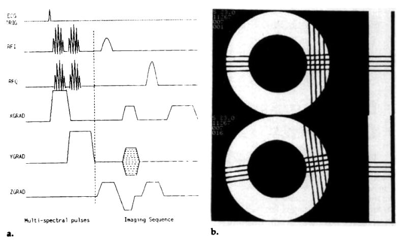
(a) A multispectral, radio-frequency pulse tagging sequence. The sinc-Hamming envelope of the tagging pulses is modulated with discrete sideband frequencies to tag a set of parallel planes simultaneously. Two multispectral pulses with orthogonal gradients were used to produce a grid. (b) A sample 4 × 4 grid of tags produced in a rotating phantom. The separation of the tag lines was 4.0 mm; the time to produce the grid pattern was 13.0 msec. The phantom experiments are explained in full in the Phantom Experiments section of the Results section.

Tag Detection

A requirement for computing the strains with MR tagging data was use of a robust method for estimating the position of the intersection points of the tags. These points were used to construct a system of equations to solve for the deformation gradient F. This process is described below in the Strain Calculation section.

We wrote computer programs with which to detect the tag intersection points. The user displayed the image on a 1,024 × 860 canvas and zoomed in on the region of the grid pattern. The user then defined a segment of a tag line by placing seed points along the tag line with a computer mouse. After the points were placed, a third-order polynomial was fit through the points. This represented the seed line from which the search for the tag was conducted. In practice, this seed line usually tracked the tag line very closely. At points along the seed line, lines perpendicular to the seed line were computed. These lines were approximately perpendicular to the tag. By using bilinear interpolation, seven points were sampled along the perpendicular lines through the tag line at a separation equal to the pixel grid. These points were fit to a model of the tag profile given by

$$a_1{e}^{-{\left(x-\text{μ}\right)}^{2/{\text{σ}}^2}}\hspace{0.17em}+\hspace{0.17em}{a}_{2}x\hspace{0.17em}+\hspace{0.17em}{a}_3.$$ (1)

The $a_1{e}^{-{(x-\text{μ})}^2/{\text{σ}}^2}$ term was the tag profile, and the a₂x + a₃ term accounted for local linear intensity changes. The center of the tag was given by the position of the mean of the gaussian curve (μ).

A new set of seed points was created in this way. The algorithm was repeated with the new seed points until convergence was reached. At completion, each tag, or a segment of each tag surrounding an intersection, was characterized by the lowest order polynomial that yielded uncorrelated residual errors. The intersection of the polynomials that made up the grid was computed, and the coordinates of the tag intersection points were written to a file for subsequent calculation of the deformation. This algorithm is outlined in Figure 2.

Figure 2.

(a) A diagram showing the components of the tag detection algorithm. The user places the initial seed points (black circles) on a zoomed image with use of a computer mouse. The dashed line shows a fit to the seed points. The solid lines perpendicular to the dashed line are the paths along which the search for the center of the tag was performed. (b) A flow chart for the algorithm used to obtain a polynomial fit to a segment of a tag line.

The estimate of the parameter μ in the gaussian curve was the position of the center of the tag line. Because the fit to the above model had few degrees of freedom, the confidence interval for the position of the center of the tag was computed by using a Monte-Carlo simulation (29).

Strain Calculation

The concepts of continuum mechanics can be used to analyze myocardial deformation (11,12,17,34). The tagging pattern applied at end diastole defines the material coordinates in the myocardium. A simple example of these coordinates is an orthogonal grid of tags. The material coordinates at the time t = 0 are said to be the reference configuration, and a position in the myocardium is designated by the vector X.

If we assume linear distortions, two particles that are an elemental distance dX apart in the reference configuration will be mapped at time t to dx in the new configuration by

$$\text{d}\text{x}\left(t\right)\hspace{0.17em}=\hspace{0.17em}F\left(\text{X},t\right)\text{dX}\text{. }$$ (2)

The distance dx is measured in the spatial coordinates, which in this case correspond to the pixel grid of the image. Equation (2) defines the deformation gradient F(X,t). For two-dimensional strains, it is a 2 × 2 matrix F_ij. Note that the deformation gradient is a function of the material coordinates X; that is, it is a function of position in the heart. If we derive the deformation gradient F(X,t) in a region of interest in the myocardium, we will have fully characterized the spatial and temporal dependence of the deformation of that region to first order. To assume that the distortions are linear, the region of the myocardium over which the measurement is made must be small. Myocardial deformations are highly nonlinear on a global scale, but on a local scale they may be approximated as linear.

Defining a tagging pattern is equivalent to defining the material coordinates of the body, whereas defining the imaging protocol was equivalent to defining the spatial coordinates. For a complete description of the deformation of a region of the myocardium, both the material coordinates and the spatial (or imaging) coordinates must span three-dimensional space. Then the deformation gradient F can be found by inverting a system of linear equations defined by Equation (2). Polar decomposition can then be used to express F as the product of a rotation and dilation matrix; the strain tensor can also be calculated (34).

A straightforward method for calculating the strain tensor was used in this study. The deformation gradient tensor gave a full description of deformation in a local region of the heart, provided that the region was small enough to enable approximation of the distortions as linear. A computer program was written to solve for the components of the deformation gradient by using the tag intersection points described above in the Tag Detection section. First, a set of N differential vectors was computed from (N + 1) tag intersection points. The reference configuration vectors ΔX were calculated from the tag intersection points in the first image. The differentials of the deformed configuration Δx were calculated from the image that showed the myocardium in the deformed state at some time t. This yielded a system of N equations

$$\text{Δ}\text{x}{\left(t\right)}_i\hspace{0.17em}=\hspace{0.17em}F\hspace{0.17em}\left(\text{X},t\right)\text{Δ}{\text{X}}_i,\hspace{0.17em}$$ (3)

where i = 1,2,…,N. The N equations were rewritten in the form

$$Av\hspace{0.17em}=\hspace{0.17em}b,\hspace{0.17em}$$ (4)

where the solution vector v comprised the components of F at the center of mass of the (N + 1) points, A comprised the components of the differential vectors in the undeformed state, and b comprised the components of the differential vectors in the deformed state. For example, if three tag intersection points were used to derive two differential vectors in both the reference configuration and the deformed configuration, Equation (4) could be written explicitly as

$$\left(\begin{array}{l}\text{Δ}{\text{X}}_1^1\text{Δ}{\text{X}}_2^{1}00\\ 00\text{Δ}{\text{X}}_1^1\text{Δ}{\text{X}}_2^1\\ \text{Δ}{\text{X}}_1^2\text{Δ}{\text{X}}_2^{2}00\\ 00\text{Δ}{\text{X}}_1^2\text{Δ}{\text{X}}_2^2\end{array}\right)\left(\begin{array}{l}{F}_{11}\\ F_{12}\\ F_{21}\\ F_{22}\end{array}\right)=\left(\begin{array}{l}\text{Δ}{x}_1^1\\ \text{Δ}{x}_2^1\\ \text{Δ}{x}_1^2\\ \text{Δ}{x}_2^2\end{array}\right),$$ (5)

where the subscripts denote components and the superscripts enumerate the vectors.

Equation (4) was inverted to solve for the components of F. If the number of differential vectors used was greater than two, a singular-value decomposition algorithm was used to solve for the F_ij. After the components of F were calculated, the strains could be calculated in any direction (11) by using the strain tensor E = ½ (F^TF – I), where F^T is the transpose of F and I is the identity matrix. Also, the principal strains and their directions were calculated by diagonalizing E.

Precision of Strain Estimates

The procedure for obtaining the strain tensor E and the principal strains was fairly complex, involving a number of nonlinear operations. Therefore, it was decided to determine the precision of the strain estimates by using a Monte-Carlo simulation (29). With this method, the calculation of the strain was repeated in many trials, with independent random noise added to the original data for each trial. The precision of the strain estimate was obtained by analyzing the statistics of the estimates from the trials.

Results

Phantom Experiments

Figure 1b shows a tagging grid in a rigidly rotating phantom at two time points. The phantom was made of two concentric Perspex cylinders filled with agar gel, with T1 = 1,655 msec ± 20 and T2 = 940 msec ± 20. The inner diameter was 50 mm and the outer diameter, 89 mm. The grid was produced in 13 msec, with two multispectral pulses; the separation of the tag lines was 4 mm. For these images, repetition time was 1,800 msec, echo time was 30 msec, and the rotation rate of the phantom was 42.4°/sec. The time between the first image and the second image was 141 msec.

The deformation gradient F was computed for each of the nine boxes contained in the tagging grid by using the four tag intersection points on the corner of the box. Each of these matrixes was decomposed into a rotation matrix R and a dilation matrix D. The dilation matrix should be the identity matrix and the rotation matrix should represent the rotation of the grid through 6.0° (42.4° sec⁻¹ · 0.141 sec). The Table shows the results from the nine boxes; these results demonstrate that under these conditions the method produced accurate and precise measures of strain.

The standard deviations calculated from these experiments were consistent with an uncertainty of 0.15–0.30 pixels (0.11–0.22 mm) in the position of the tag intersection points. These estimates of the uncertainty were obtained from the relationship predicted between the uncertainty of F₁₁ and the uncertainty of the tag point position. Figure 3 shows a plot of the error in F₁₁ as a function of the input uncertainty (28) in the coordinates. This relation was derived by using the Monte-Carlo simulation. This method can be used to estimate the confidence intervals on any parameter calculated from the tagging data, such the components of the strain tensor E and the principal strains.

Figure 3.

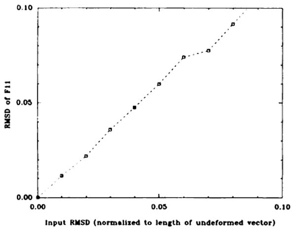
A plot of the expected uncertainty in F₁₁ versus the root-mean-squared deviation of the position of the tag points (normalized to the length of the differential ΔX). The data were obtained from a Monte-Carlo simulation in which 400 independent data sets for each input noise level were used to calculate F. This root-mean-squared deviation on the components of F were calculated from these 400 trials. RMSD = root-mean-squared deviation.

In Vivo Data

To test the feasibility of measuring strains in the myocardium with MR tagging techniques, we performed an experiment in a normal dog. The dog, which weighed 10 kg, was anesthetized with 65 mg/mL intravenously administered pentobarbital, after pre-anesthetic intramuscular administration of 1 mL of 10 mg/mL acepromazine. A level of anesthesia was maintained such that mechanical ventilation was not required. Three surface electrode leads were placed after small regions on the right leg, the right side of the chest, and the right shoulder were shaved. The dog was placed on its side in the extremity coil, which was used for transmission and reception. The dog's front legs, head, and back legs extended outside the coil and were supported with padding.

Figure 4 shows grid-tag images at nine time points through systole in a normal dog heart, with a temporal resolution of 30 msec. The first image was obtained 25 msec after the initial upslope of the R wave of the QRS complex triggered the tagging pulses (Fig 1a). The heart rate of the dog was 100 beats pen minute. The voxel dimensions of the images were 0.6 ×1.2 × 5.0 mm, collected with a 256 × 128 matrix and four signals averaged. The total imaging time was 46 minutes. The tag lines, separated by 4.0 mm, were produced with multispectral radio-frequency pulses, as described above (Pulse Sequence Design section), with a modification that produced a 2 × 4 grid of lines.

Figure 4.

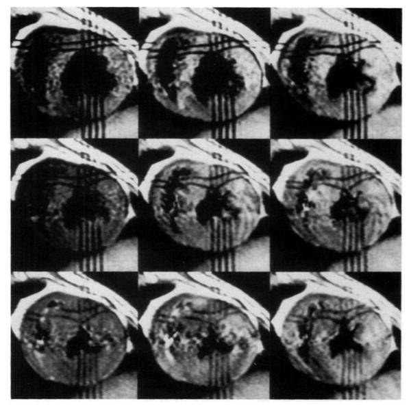
In vivo data produced with the multispectral radio-frequency pulse tagging sequence. Nine time points (25, 55, 85, 115, 145, 175, 205, 235, 265 msec) were measured through the systolic interval in the normal dog. (t = 0 was at the initial upslope of the R wave in the QRS complex.) The voxel dimensions were 0.6 × 1.2 × 5.0 mm, collected with a 256 × 128 matrix and four signals averaged. The phase-encoding direction was horizontal in these images. The total imaging time was 46 minutes. The tags were separated by 4.0 mm.

Tag detection

Figure 5a shows a line through a tag from the 175-msec image seen in Figure 4. Figure 5b shows a plot of pixel intensities along this line. Also shown is the model fit to the tag profile; it is a gaussian curve profile, with a linear ramp for the baseline as described above (Tag Detection section in Materials and Methods). Figure 5c shows a plot of the squared error between the model and the pixel intensities as the value of μ (the mean of the gaussian curve) is shifted. The sharp minimum in this function implies that this is a very sensitive way of determining the center of the tag line. The confidence interval on the determination of the center of the tag was ±0.2 mm for the case shown in Figure 5, which is a tag with relatively low contrast due to T1 decay. This confidence interval was calculated by using a Monte-Carlo simulation of this fitting procedure (29) and was found to be relatively insensitive to the values of a₁ and σ, as long as these values were larger than their value at the minimum squared-error fit.

Figure 5.

(a) A zoomed image of the grid-tag pattern in the 175-msec image seen in Figure 4. A line is drawn along a direction perpendicular to the tag. (b) A plot of pixel intensities through the tag, along the line shown in a. The solid line shows the model function, $a_1{e}^{-{(x-\text{μ})}^2/{\text{σ}}^2}+a_{2}x+a_3$, fit to the tag. The error bars represent the root-mean-squared deviation measured in the heart wall; this error therefore includes the nonuniform heart wall signal and the random signal from flow artifact. (c) A plot of the squared error between the model and the pixel values versus the position of the mean of the gaussian curve (μ). Notice the sharp definition of the minimum.

The noise level used in the Monte-Carlo simulation was the measured root-mean-squared deviation on the adjacent nontagged myocardium. This deviation included the effect of nonuniform signal from the myocardium and the superimposed flow artifact, so it represented an upper bound. This root-mean-squared deviation was found to be greater than the measured background noise (35) by a factor of two. A Monte-Carlo simulation was required to calculate the precision of the estimate of μ because of the low number of degrees of freedom in the fit.

The preliminary results from this experiment indicated that the position of the center of the tag could be determined to within less than ±0.1 mm for the end-diastolic image (high-contrast tags) and to within less than ±0.2 mm for the end-systolic images (lower-contrast tags). This rivals the precision obtained when measuring the position of metallic beads with biplane cineradiography (2,18).

The positions of the center of the tag line were fit to a straight line in the immediate region (±2 mm) around the intersection of two tag lines; the tag intersection points were found by computing the intersection of these straight lines. The error in the position of the intersection points was computed by using standard propagation of errors techniques (36).

One-dimensional strain

The simplest method of computing strain was to measure the change in length between two markers in the medium. Two tag intersection points could be used to measure this length. The one-dimensional strain (34) was an analogue of the two-dimensional strain E given above (Strain Calculation section in Materials and Methods):

$$E\hspace{0.17em}\hspace{0.17em}\frac{1}{2}\left(\frac{l^2\left(t\right)\hspace{0.17em}-\hspace{0.17em}{l}_0^2}{l_0^2}\right).\hspace{0.17em}$$ (6)

Figure 6a shows the strain in the circumferential direction as a function of time. This was computed from the two tag-intersection points shown in Figure 4 at the upper left corner and at the lower right corner of the tagging grid. Therefore, this plot reflects the average circumferential strain over the region between these points. Figure 6b shows the strain in the radial direction computed from the two tag intersection points at the bottom left and top right of the central box in the tagging grid. These graphs demonstrate that a 30-msec temporal resolution is adequate for measuring the change in the strain through the systolic interval.

Figure 6.

(a) A plot of the circumferential strain as a function of time. The strain was calculated as $½\left\{[l^2\left(t\right)-l_0^2]/l_0^2\right\}$, where l₀ is the distance between the top left corner and bottom right corner of the tagging grid shown in the 25-msec image seen in Figure 4, and l(t) is the distance between those two points in the images at later times t. The error was computed from simple error propagation techniques by using the estimated error on l₀ and l(t) obtained from the tag detection algorithm. (b) A plot of the radial strain as a function of time. The strain was calculated as in a, but the two points used were the top right and bottom left corners of the central box in the tagging grid seen in Figure 4.

Two-dimensional strain

A higher-resolution calculation of the two-dimensional strain was performed by using the four points that define the central box in the tagging grid seen in Figure 4. Figure 7 shows a diagram of the changing shape of this box at three time points through the systolic interval. These diagrams were derived from the detected tag intersection points.

Figure 7.

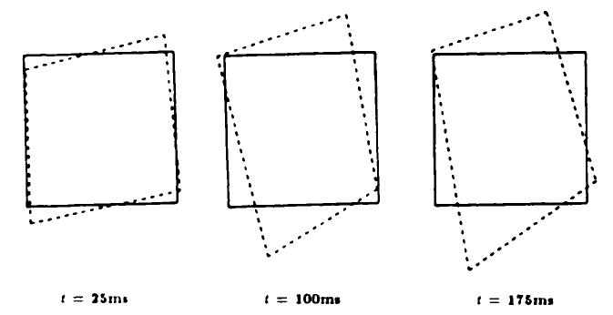
Deformation of the central box in the tagging grid seen in Figure 4 is shown at three different times.

The solid-line boxes represent the shape of the original tagging grid. The deformation gradient F was calculated for four “tiles” in this box. (A tile was defined as the region bounded by two sides and a diagonal of the box.) Figure 8 shows how a circle would be deformed if it was at the center of mass of the tile. The lengths of the semimajor and semiminor axes of the ellipse represent the values of the principal components of the dilation matrix D. The orientation of the ellipse is given by the angle of the rotation matrix R. This is the most direct visual representation of the deformation.

Figure 8.

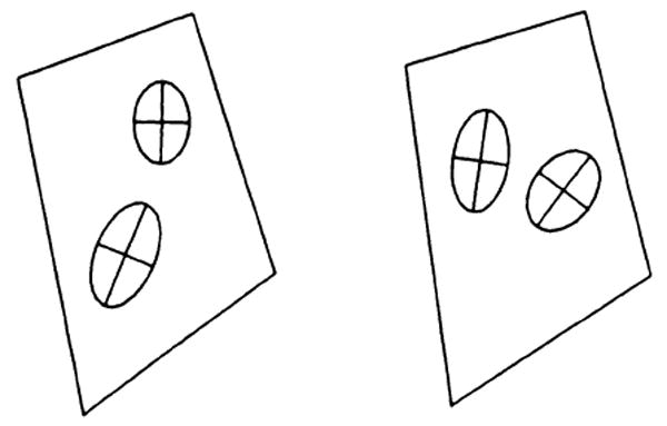
A graphic demonstration of the value of the strain in this box at the time t = 175 msec. Each ellipse shows how a circle at that location would deform. Note the transmural gradient in this strain.

In Figure 8, note the marked difference in the strain at the endocardium (bottom left) versus the strain at the center of the heart wall (top right). The confidence intervals derived for the position of the tag intersection points were used in a Monte-Carlo simulation to derive the confidence intervals for the principal strain vector. In this example, difference in the principle strain vector was detected with a P < .01. This is evidence that we can detect transmural gradients in the strain by using this technique.

Discussion

An important aspect of measuring strain in the myocardium is the need to obtain sufficiently high resolution. It has been shown by Gallagher et al (6) that there is a complex and non-uniform response in the perfusion and strain in the heart wall under conditions of partial stenosis of the circumflex coronary artery. The subendocardial layer of the heart wall is more sensitive to partial stenosis than is the epicardial layer. To obtain the maximum sensitivity to regional ischemia, the strain must be measured with high resolution and in any direction.

The strain estimates reported herein are two-dimensional. A full three-dimensional strain tensor is required to completely characterize the strain field in the heart wall. Computing this strain tensor would require that data be obtained that measured the translation of the tissue through the imaging section. The strain estimates reported herein are computed under the assumption that the strain does not vary greatly as a function of displacement perpendicular to the imaging section. Preliminary results in which biplane tagging data have been obtained indicate that this assumption is valid for the data used in this study.

It is important when computing two-dimensional strains from tagging grids obtained in a single plane that no reference to the endocardial or epicardial wall be used. It is tempting to use the intersection of a tag line with the heart wall as a tag intersection point. However, the distance between the tagging planes and the heart wall will be a highly variable function of the position of the short-axis section because the heart wall is curved. The distance between parallel tags will not be a function of position of the short-axis section. This is shown schematically in Figure 9. Therefore, the use of only tag intersection points is a requirement for computing two-dimensional strains without the use of orthogonal images to track the translation of the section that is used as the reference configuration.

Figure 9.

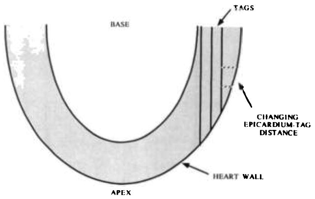
A diagram shows how the distance between the tagging planes and the epicardium can change rapidly as a function of position. This diagram shows a long-axis view of the heart. The dashed lines show the distance between the tag planes and the epicardium.

Local tagging grids were produced for this study. Development of specialized high-power radio-frequency coils and rapidly switching gradients will make it possible to produce high-resolution tagging grids over the entire myocardium (32,37).

In this study, we tested the accuracy and precision of an MR tagging technique for measuring strain with a spatial resolution of approximately 2 mm. An experiment was performed in a normal dog to demonstrate the feasibility of obtaining strain measurements in the beating heart by using this method. A tag detection algorithm was developed with which the center of a tag line could be measured with a precision that ranged 0.1–0.2 mm over the systolic interval. A transmural gradient in the principal strain of the normal dog heart was detected.

Comparison of Measured and Expected Values of Dilation Matrix D and Rotation Angle

Parameter Measured	Expected Value	Measured Value	Standard Deviation
D11	1.0	1.01	0.02
D12 = D21	0.0	0.00	0.02
D22	1.0	0.99	0.05
Rotation (degrees)	6.0	6.0	1.2

Note. — The measured values are the mean from nine boxes in Figure 1b; the standard deviation is computed from the nine estimates and this mean.

References

- 1.Zerhouni EA, Parish DM, Rogers WJ, Yang A, Shapiro EP. Human heart tagging with MR imaging: a method for noninvasive assessment of myocardial motion. Radiology. 1988;169:59–63. doi: 10.1148/radiology.169.1.3420283. [DOI] [PubMed] [Google Scholar]
- 2.Hunter WC, Zerhouni EA. Imaging distinct points in left ventricular myocardium to study regional wall deformation. In: Anderson JH, editor. Innovations in diagnostic radiology. Berlin: Springer-Verlag; 1989. [Google Scholar]
- 3.Ingels NB, Daughters GT, Stinson EB, Alderman EL. Measurement of midwall myocardial dynamics in intact man by radiography of surgically implanted markers. Circulation. 1975;52:859–867. doi: 10.1161/01.cir.52.5.859. [DOI] [PubMed] [Google Scholar]
- 4.LeWinter MM, Kent RS, Kroener JM, Carew TE, Covell JW. Regional differences in myocardial performance in the left ventricle of the dog. Circ Res. 1975;37:191–199. doi: 10.1161/01.res.37.2.191. [DOI] [PubMed] [Google Scholar]
- 5.Sabbah HN, Marzilli M, Stein PD. The relative role of subendocardium and subepicardium in left ventricular mechanics. Am J Physiol. 1981;240:H920–H926. doi: 10.1152/ajpheart.1981.240.6.H920. [DOI] [PubMed] [Google Scholar]
- 6.Gallagher KP, Osakada G, Matsuzaki M, Miller M, Kemper WS, Ross J. Subepicardial segmental function during coronary stenosis and the role of myocardial fiber orientation. Circ Res. 1982;50:352–359. doi: 10.1161/01.res.50.3.352. [DOI] [PubMed] [Google Scholar]
- 7.Gallagher KP, Osakada G, Matsuzaki M, Miller M, Kemper WS, Ross J. Nonuniformity of inner and outer systolic wall thickening in conscious dogs. Am J Physiol. 1985;249:H241–H248. doi: 10.1152/ajpheart.1985.249.2.H241. [DOI] [PubMed] [Google Scholar]
- 8.Arts T, Veenstra PC, Reneman RN. Epicardial deformation and left ventricular wall mechanics during ejection in the dog. Am J Physiol. 1982;243:H379–H390. doi: 10.1152/ajpheart.1982.243.3.H379. [DOI] [PubMed] [Google Scholar]
- 9.Myers JH, Stirling MC, Choy M, Buda AJ, Gallagher KP. Direct measurement of inner and outer wall thickening dynamics with epicardial echocardiography. Circulation. 1986;74:164–172. doi: 10.1161/01.cir.74.1.164. [DOI] [PubMed] [Google Scholar]
- 10.Fenton TR, Cherry JM, Klassen GA. Transmural myocardial deformation in the canine left ventricular wall. Am J Physiol. 1980;235:319–329. doi: 10.1152/ajpheart.1978.235.5.H523. [DOI] [PubMed] [Google Scholar]
- 11.Meier GD, Ziskin MC, Santamore WP, Bove AA. Kinematics of the beating heart. IEEE Trans Biomed Eng. 1980;27:319–329. doi: 10.1109/TBME.1980.326740. [DOI] [PubMed] [Google Scholar]
- 12.Meier GD, Bove AA, Wantamore WP. Contractile function in canine right ventricle. Am J Physiol. 1980;239:H794–H804. doi: 10.1152/ajpheart.1980.239.6.H794. [DOI] [PubMed] [Google Scholar]
- 13.Shoukas AA, Sagawa K, Maughan WL. Chronic implantation of radiopaque beads on endocardium, midwall, and epicardium. Am J Physiol. 1981;241:H104–H107. doi: 10.1152/ajpheart.1981.241.1.H104. [DOI] [PubMed] [Google Scholar]
- 14.Garrison JB, Ebert WL, Jenkins RE, et al. Measurement of three-dimensional positions and motions of large numbers of spherical radiopaque markers from biplane cineradiograms. Comput Biomed Res. 1982;15:76–96. doi: 10.1016/0010-4809(82)90054-4. [DOI] [PubMed] [Google Scholar]
- 15.Walley KR, Grover M, Raff GL, Benge W, Hannaford B, Glantz SA. Left ventricular dynamic geometry in the intact and open chest dog. Circ Res. 1982;50:573–589. doi: 10.1161/01.res.50.4.573. [DOI] [PubMed] [Google Scholar]
- 16.Waldman LK, Fung YC, Covell JO. Transmural myocardial deformation in the canine left ventricle. Circ Res. 1985;57:152–163. doi: 10.1161/01.res.57.1.152. [DOI] [PubMed] [Google Scholar]
- 17.Waldman LK, Nosand D, Villareal F, Covell JW. Relation between transmural deformation and local myofiber direction in the canine left ventricle. Circ Res. 1988;63:550. doi: 10.1161/01.res.63.3.550. [DOI] [PubMed] [Google Scholar]
- 18.Hunter WC, Douglas AS, Sagawa Y, Holmes JW, Rodriguez EK. Local strains in lv myocardium: uniquely determined by volume during ejection (abstr)? Circulation. 1988;78(2):224. [Google Scholar]
- 19.McVeigh ER, Zerhouni EA. Book of Abstracts: Society of Magnetic Resonance in Medicine 1989. Berkeley, Calif: Society of Magnetic Resonance in Medicine; 1989. A rapid starburst sequence for cardiac tagging (abstr) p. 53. [Google Scholar]
- 20.Bolster B, McVeigh ER, Zerhouni EA. Myocardial tagging in polar coordinates with striped tags. Radiology. 1990;177:769–772. doi: 10.1148/radiology.177.3.2243987. [DOI] [PMC free article] [PubMed] [Google Scholar]
- 21.Buchalter MB, Weiss JL, Rogers WJ, et al. Noninvasive quantification of left ventricular rotational deformation in normal humans using magnetic resonance imaging myocardial tagging. Circulation. 1990;81:1236–1244. doi: 10.1161/01.cir.81.4.1236. [DOI] [PubMed] [Google Scholar]
- 22.Shapiro EP, Buchalter MB, Rogers WJ, Zerhouni EA, Guier WH, Weiss JL. LV twist is greater with inotropic stimulation and less with regional ischemia (abstr) Circulation. 1988;78(2):466. [Google Scholar]
- 23.Rogers WJ, Buchalter MB, Weiss JL, et al. Selective NMR tracking of a slice of human heart through the cardiac cycle (abstr) Circulation. 1988;78(2):591. [Google Scholar]
- 24.Lima J, Weiss J, Lessick J, et al. Dysfunction of the adjacent nonischemic zone: is end-systolic stress increased (abstr)? Circulation. 1989;80(2):98. [Google Scholar]
- 25.Lima J, Bouton S, Zerhouni E, et al. Nonischemic adjacent dysfunction is greatest in the subendocardium during ischemia (abstr) Circulation. 1989;80(2):97. [Google Scholar]
- 26.Lima J, Jeremy R, Guier W, et al. Accurate systolic thickening by three-dimensional MRI: correlation with sonomicrometers in normal and ischemic myocardium (abstr) Circulation. 1990;82(3):762. [Google Scholar]
- 27.Zerhouni EA, McVeigh ER, Bouton S, Bolster B, Shapiro E, Weiss J. Dynamic three-dimensional tagged imaging of left ventricular contraction (abstr) Radiology. 1990;177(P):101. [Google Scholar]
- 28.McVeigh ER, Yang A, Hill G, Zerhouni EA. Book of abstracts: Society of Magnetic Resonance in Medicine 1990. Berkeley, Calif: Society of Magnetic Resonance in Medicine; 1990. Accuracy of strain measurements with tagging methods (abstr) p. 1009. [Google Scholar]
- 29.Press WH, Flannery BP, Teukolsky SA, Vetterling WT. Numerical recipes: the art of scientific computing. Vol. 360. Cambridge: Cambridge University Press; 1988. p. 548. [Google Scholar]
- 30.Axel L, Dougherty L. MR imaging of motion with spatial modulation of magnetization. Radiology. 1989;171:841–849. doi: 10.1148/radiology.171.3.2717762. [DOI] [PubMed] [Google Scholar]
- 31.Axel L, Dougherty L. Heart wall motion: improved method of spatial modulation of magnetization for MR imaging. Radiology. 1989;172:349–350. doi: 10.1148/radiology.172.2.2748813. [DOI] [PubMed] [Google Scholar]
- 32.Mosher TJ, Smith MB. A DANTE tagging sequence for the evaluation of translational sample motion. J Magn Reson. 1990;15:334–339. doi: 10.1002/mrm.1910150215. [DOI] [PubMed] [Google Scholar]
- 33.Hennig J, Friedburg H. Book of abstracts: Society of Magnetic Resonance in Medicine 1989. Berkeley, Calif: Society of Magnetic Resonance in Medicine; 1989. Imaging of heart wall motion using MR-interferography (abstr) p. 53. [Google Scholar]
- 34.Malvern LE. Introduction to the mechanics of a continuous medium. Englewood Cliffs, NJ: Prentice Hall; 1969. [Google Scholar]
- 35.Henkelman RM. Measurement of signal intensities in the presence of noise in MR images. Med Phys. 1985;12:232–236. doi: 10.1118/1.595711. [DOI] [PubMed] [Google Scholar]
- 36.Bevington PR. Data reduction and error analysis for the physical sciences. New York: McGraw-Hill; 1969. [Google Scholar]
- 37.Bolster B, McVeigh E, Schoeniger J, Zerhouni E. Book of abstracts: Society of Magnetic Resonance in Medicine 1990. Berkeley, Calif: Society of Magnetic Resonance in Medicine; 1990. Efficient production of high resolution tagging grids with sinc modulated comb functions (abstr) p. 1115. [Google Scholar]