Abstract
For taxonomic levels higher than species, the abundance distributions of the number of subtaxa per taxon tend to approximate power laws but often show strong deviations from such laws. Previously, these deviations were attributed to finite-time effects in a continuous-time branching process at the generic level. Instead, we describe herein a simple discrete branching process that generates the observed distributions and find that the distribution's deviation from power law form is not caused by disequilibration, but rather that it is time independent and determined by the evolutionary properties of the taxa of interest. Our model predicts—with no free parameters—the rank-frequency distribution of the number of families in fossil marine animal orders obtained from the fossil record. We find that near power law distributions are statistically almost inevitable for taxa higher than species. The branching model also sheds light on species-abundance patterns, as well as on links between evolutionary processes, self-organized criticality, and fractals.
Taxonomic abundance distributions have been studied since the pioneering work of Yule (1), who proposed a continuous-time branching process model to explain the distributions at the generic level and found that they were power laws in the limit of equilibrated populations. Deviations from the geometric law were attributed to a finite-time effect, namely, to the fact that the populations had not reached equilibrium. Much later, Burlando (2, 3) compiled data that seemed to corroborate the geometric nature of the distributions, even though clear violations of the law are visible in his data also. In this article, we present a model that is based on a discrete branching process whose distributions are time independent and in which violations of the geometric form reflect specific environmental conditions and pressures to which the assemblage under consideration was subjected during evolution. As such, the model holds the promise that an analysis of taxonomic abundance distributions may reveal certain characteristics of ecological niches long after their inhabitants have disappeared.
The model described herein is based on the simplest of branching processes, known in the mathematical literature as the Galton–Watson process. Consider an assemblage of taxa at one taxonomic level. This assemblage can be all the families under a particular order, all the subspecies of a particular species, or any other group of taxa at the same taxonomic level that can be assumed to have suffered the same evolutionary pressures. We are interested in the shape of the rank-frequency distribution of this assemblage and the factors that influence it.
We describe the model by explaining a specific example: the distribution of the number of families within orders for a particular phylum. The adaptation of this model to different levels in the taxonomic hierarchy is obvious. We can assume that the assemblage was founded by one order in the phylum and that this order consisted of one family that had one genus with one species. We further assume that new families in this order are created by means of mutation in individuals of extant families. This creation of new families can be viewed as a process by which existing families can “replicate” and create new families of the same order, which we term daughters of the initial family. Of course, relatively rarely, mutations may lead to the creation of a new order, a new class, etc. We define a probability Pi for a family to have i daughter families of the same order (true daughters). Thus, a family will have no true daughters with probability P0, one true daughter with probability P1, and so on. For the sake of simplicity, we initially assume that all families of this phylum share the same Pi. We show later that variance in Pi among different families does not significantly affect the results, in particular the shape of the distribution. The branching process described above gives rise to an abundance distribution of families within orders, and the probability distribution of the branching process can be obtained from the Lagrange expansion of a nonlinear differential equation (4). Using a simple iterative algorithm (http://xxx.lanl.gov/abs/cond-mat/9903085) in place of this Lagrange expansion procedure, we can calculate rank-frequency curves for many different sets of Pi. It should be emphasized here that we are mostly concerned with the shape of this curve for n ≤ 104 and not the asymptotic shape as n → ∞, a limit that is not reached in nature.
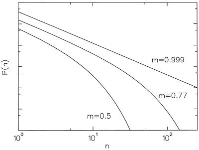
For different sets of Pi, the theoretical curve can be close to a power law, a power law with an exponential tail, or a purely exponential distribution (Fig. 1). We show herein that there is a global parameter that distinguishes among these cases. Indeed, the mean number of true daughters (i.e., the mean number of different families of the same order to which each family gives rise in the example above),
 |
1 |
is a good indicator of the overall shape of the curve. Universally, m = 1 leads to a power law for the abundance distribution. The further m is away from 1, the further the curve diverges from a power law and toward an exponential curve. The value of m for a particular assemblage can be estimated from the fossil record allowing for a characterization of the evolutionary process with no free parameters. Indeed, if we assume that the number of families in this phylum existing at one time is roughly constant or that this number varies slowly compared with the average rate of family creation (an assumption the fossil record seems to vindicate; ref. 5), we find that m can be related to the ratio Ro/Rf of the rates of creation of orders and families by
 |
2 |
to leading order (http://xxx.lanl.gov/abs/cond-mat/9903085).
Figure 1.
Predicted abundance pattern P(n) (probability for a taxon to have n subtaxa) of the branching model with different values of m. The curves have been individually rescaled.
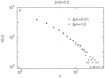
In general, we cannot expect all the families within an order to share the same m. Interestingly, it turns out that even if the Pi and m differ widely between different families, the rank-frequency curve is identical to that obtained by assuming a fixed m equal to the average of m across the families (Fig. 2), i.e., the variance of the Pi across families seems to be completely immaterial to the shape of the distribution—only the average μ ≡ 〈m〉 counts.
Figure 2.
Abundance patterns obtained from two sets of numerical simulations of the branching model, each with μ = 〈m〉 = 0.5. Different values for m were chosen from a uniform probability distribution of width 1 for the runs represented by crosses and from a distribution of width 0.01 for those represented by circles. Simulations in which m and Pi are allowed to vary significantly and those where they are severely constricted are impossible to distinguish if they share the same 〈m〉.
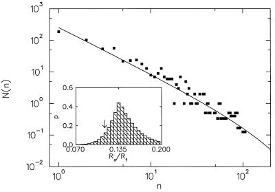
In Fig. 3, we show the abundance distribution of families within orders for fossil marine animals (6), together with the prediction of our branching model. The theoretical curve was obtained by assuming that the ratio Ro/Rf is approximated by the ratio of the total number of orders to the total number of families,
 |
3 |
and that both are very small compared with the rate of mutations. The prediction μ = 0.9(16) obtained from the branching process model by using Eq. 3 as the sole parameter fits the observed data remarkably well (P = 0.12; Kolmogorov–Smirnov test; see Fig. 3 Inset). Alternatively, we can use a best fit to determine the ratio Ro/Rf without resorting to Eq. 3, yielding Ro/Rf = 0.115(20) (P = 0.44). Fitting abundance distributions to the branching model thus allows us to determine a ratio of parameters that reflect dynamics intrinsic to the taxon under consideration and the niche(s) it inhabits. Indeed, some taxa analyzed in refs. 2 and 3 are better fit with 0.5 < μ < 0.75, pointing to conditions in which the rate of taxon formation was much closer to the rate of subtaxon formation, indicating either a more “robust” genome or richer and more diverse niches.
Figure 3.
The abundance distribution of fossil marine animal orders (6) (squares) and the predicted curve from the branching model (solid line). The fossil data have been binned above n = 37 with a variable bin size (http://xxx.lanl.gov/abs/cond-mat/9903085). The predicted curve was generated by using Ro/Rf = No/Nf = 0.115, where No and Nf were obtained directly from the fossil data. (Inset) Kolmogorov–Smirnov significance levels P obtained from comparison of the fossil data to several predicted distributions with different values of Ro/Rf, showing that the data are best fit by Ro/Rf = 0.135. The arrow points to our prediction Ro/Rf = 0.115 where P = 0.12. A Monte Carlo analysis shows that for a sample size of 626 (as we have here), the predicted Ro/Rf = 0.115 is within the 66% confidence interval of the best fit Ro/Rf = 0.135 (P = 0.44). The Kolmogorov–Smirnov tests were done after removal of the first point, which suffers from sampling uncertainties.
In general, however, Burlando's data (2, 3) suggest that a wide variety of taxonomic distributions are fit quite well by power laws (μ = 1), implying that actual taxonomic abundance patterns from the fossil record are characterized by a relatively narrow range of μ near 1. Such distributions are indeed likely within the model description advanced here. It is obvious that μ cannot remain above 1 for significant time scales, because it would lead to an infinite number of subtaxa for each taxon. What about low μ? We propose that low values of μ are not observed for large (and therefore statistically important) taxon assemblages for the following reasons. A small value of μ implies either a small number of total individuals for this assemblage or a very low rate of beneficial taxon-forming (or niche-filling) mutations. The former might lead to this assemblage not being recognized at all in field observations. Either case will lead to an assemblage with too few taxa to be statistically tractable. Also, because such an assemblage contains a small number of individuals or is less suited for further adaptation or both, it would seem to be susceptible to early extinction.
The branching model can—with appropriate care—also be applied to species-abundance distributions, even though these are more complicated than those for higher taxonomic orders for several reasons. Among these are the effects of sexual reproduction and the localized and variable effects of the environment and other species on specific populations. Still, because the arguments for using a branching process model essentially rely on mutations that may produce lines of individuals that displace others, species-abundance distributions may turn out not to be qualitatively as different from taxonomically higher-level rank-frequency distributions as is usually expected.
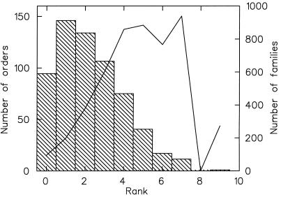
Historically, species abundance distributions have been characterized by using frequency histograms of the number of species in logarithmic abundance classes. For many taxonomic assemblages, this procedure was found to produce a humped distribution truncated on the left—a shape usually dubbed lognormal (7–10). In fact, this distribution is not incompatible with the power law type distributions described above. Indeed, plotting the fossil data of Fig. 3 in logarithmic abundance classes produces a lognormal shape (Fig. 4). For species, μ is the mean number of children each individual of the species has. (Of course, for sexual species, μ would be half the mean number of children per individual.) In the present case, μ < 1 implies that extant species' populations decrease on average, whereas μ = 1 implies that average populations do not change. An extant species' population can decline because of the introduction of competitors and/or the decrease of the size of the species' ecological niche. Let us examine the former more closely. If a competitor is introduced into a saturated niche, all species currently occupying that niche would temporarily see a decrease in their m until a new equilibrium was obtained. If the new species is significantly fitter than the previously existing species, it may eliminate the others. If the new species is significantly less fit, then it may be the one eliminated. If the competitors are about as efficient as the species already present, then the outcome is less certain. Indeed, it is analogous to a nonbiased random walk with a possibility of ruin. The effects of introducing a single competitor are transient. However, if new competitors are introduced more or less periodically, then these added competitors would act to push m lower for all species in this niche, and we would expect an abundance pattern closer to the exponential curve as opposed to the power law than otherwise expected. We have examined this question in simulations of populations in which new competitors were introduced into the population by means of neutral mutations—mutations leading to new species of the same fitness as extant species—and found that these distributions are fit very well by the branching model. A higher rate of neutral mutations and thus of new competitors leads to distributions closer to exponential. We have performed the same experiment in more sophisticated systems of digital organisms (artificial life; refs. 11 and 12) and found the same result (http://xxx.lanl.gov/abs/cond-mat/9903085).
Figure 4.
The abundance distribution of fossil marine animal orders in logarithmic abundance classes (the same data shown in Fig. 3). The histogram shows the number of orders in each abundance class (left scale), whereas the solid line depicts the number of families in each abundance class (right scale). Species rank-abundance distributions where the highest abundance class present also has the highest number of individuals (as in these data) are termed canonical lognormal (8, 9).
If no new competitors are introduced but the size of the niche is gradually reduced, we expect the same effect on m and on the abundance distributions. Whether it is possible to separate the effects of these two mechanisms in ecological abundance patterns obtained from field data is an open question. An analysis of such data to examine these trends would certainly be very interesting.
Thus far, we have sidestepped the difference between historical and ecological distributions. For the fossil record, the historical distribution we have modeled here should work well. For field observations where only currently living groups are considered, the nature of the death and extinction processes for each group will affect the abundance pattern. In our simulations and artificial-life experiments, we have universally observed a strong correlation between the shapes of historical and ecological distributions. We believe this correspondence will hold in natural distributions as well when death rates are affected mainly by competition for resources. The model's validity for different scenarios is an interesting question, which could be answered by comparison with more taxonomic data.
Our branching process model allows us to reexamine the question of whether any type of special dynamics—such as self-organized criticality (13, 14)—is at work in evolution (15, 16). Although showing that the statistics of taxon rank-frequency patterns in evolution are closely related to the avalanche sizes in self-organized criticality sandpile models, the present model clearly shows that instead of a subsidiary relationship in which evolutionary processes may be self-organized critical, the power law behavior of both evolutionary and sandpile distributions can be understood in terms of the mechanics of a Galton–Watson branching process (http://xxx.lanl.gov/abs/cond-mat/9903085 and ref. 17). The mechanics of this branching process are such that the branching trees are probabilistic fractal constructs. However, the underlying stochastic process responsible for the observed behavior can be explained simply in terms of a random walk (18). For evolution, the propensity for near power law behavior is found to stem from a dynamical process in which μ ≈ 1 is selected for and highly more likely to be observed than other values, whereas the “self-tuning” of the self-organized criticality models is seen to result from arbitrarily enforcing conditions that would correspond to the limit Ro/Rf → 0 and therefore m → 1 (http://xxx.lanl.gov/abs/cond-mat/9903085).
Acknowledgments
We thank J. J. Sepkoski for kindly sending us his amended data set of fossil marine animal families. Access to the intel paragon xp/s was provided by the Center of Advanced Computing Research at the California Institute of Technology. This work was supported by a grant from the National Science Foundation.
Footnotes
This paper was submitted directly (Track II) to the PNAS office.
References
- 1.Yule G U. Proc R Soc London Ser B. 1924;213:21–87. [Google Scholar]
- 2.Burlando B. J Theor Biol. 1990;146:99–114. [Google Scholar]
- 3.Burlando B. J Theor Biol. 1993;163:161–172. doi: 10.1006/jtbi.1993.1114. [DOI] [PubMed] [Google Scholar]
- 4.Harris T E. The Theory of Branching Processes. Berlin: Springer; 1963. [Google Scholar]
- 5.Raup D M. Paleobiology. 1985;11:42–52. [Google Scholar]
- 6.Sepkoski J J. A Compendium of Fossil Marine Animal Families. 2nd Ed. WI: Milwaukee Public Museum; Milwaukee; 1992. [PubMed] [Google Scholar]
- 7.Preston F W. Ecology. 1948;29:255–283. [Google Scholar]
- 8.Preston F W. Ecology. 1962;43:410–432. [Google Scholar]
- 9.Preston F W. Ecology. 1962;43:185–215. [Google Scholar]
- 10.Sugihara G. Am Nat. 1980;116:770–787. doi: 10.1086/283669. [DOI] [PubMed] [Google Scholar]
- 11.Adami C. Introduction to Artificial Life. New York: Springer; 1998. [Google Scholar]
- 12.Chu J, Adami C. In: Artificial Life V: Proceedings of the Fifth International Workshop on the Synthesis and Simulation of Living Systems. Langton C G, Shimohara K, editors. Cambridge, MA: MIT Press; 1997. pp. 462–469. [Google Scholar]
- 13.Bak P, Tang C, Wiesenfeld K. Phys Rev Lett. 1987;59:381–384. doi: 10.1103/PhysRevLett.59.381. [DOI] [PubMed] [Google Scholar]
- 14.Bak P, Tang C, Wiesenfeld K. Phys Rev A. 1988;38:364–374. doi: 10.1103/physreva.38.364. [DOI] [PubMed] [Google Scholar]
- 15.Sneppen K, Bak P, Flyvbjerg H, Jensen M H. Proc Natl Acad Sci USA. 1995;92:5209–5213. doi: 10.1073/pnas.92.11.5209. [DOI] [PMC free article] [PubMed] [Google Scholar]
- 16.Adami C. Phys Lett A. 1995;203:29–32. [Google Scholar]
- 17.Vespignani A, Zapperi S. Phys Rev E. 1998;57:6345–6362. [Google Scholar]
- 18.Spitzer F. Principles of Random Walk. New York: Springer; 1964. [Google Scholar]


