Modeling Nonlinear Dose-Response Relationships in Epidemiologic Studies: Statistical Approaches and Practical Challenges

Abstract

Non-linear dose response relationships pose statistical challenges for their discovery. Even when an initial linear approximation is followed by other approaches, the results may be misleading and, possibly, preclude altogether the discovery of the nonlinear relationship under investigation. We review a variety of straightforward statistical approaches for detecting nonlinear relationships and discuss several factors that hinder their detection. Our specific context is that of epidemiologic studies of exposure-outcome associations and we focus on threshold and J-effect dose response relationships. The examples presented reveal that no single approach is universally appropriate; rather, these (and possibly other) nonlinearities require for their discovery a variety of both graphical and numeric techniques.

1. INTRODUCTION

The practice of fitting linear models to associations such as those relating exposures and health, is well appreciated as an approximation, as nature is rarely so simple. Thus, implicit in the fitting of linear models to observed phenomena is the belief that, despite their inherent inaccuracies, valuable insights will be revealed nonetheless. Often, the linear approximation methodology is accompanied by some combination of the fitting of selected model refinements suggested by regression diagnostics, the inclusion of additional covariates, and case analysis. In this report, we reason that, while the practice of entertaining linear models is often appropriate, there are important non-linearities in nature for which the linear approximation is an uninformative (and possibly misleading) first analysis step. We argue that even the application of additional, more flexible, approaches might also fail to detect certain nonlinear relationships.

Our focus is on threshold and U- or J-shaped relationships where the outcome is binary (such as the occurrence or non-occurrence of a single health outcome), as these are often of interest in epidemiological investigations of dose response relationships. In the estimation of such relationships (and relationships generally), the extent to which study conclusions will be uninformative depends on the degree of disparity between the misspecified and true relationships. Less well appreciated, however, is that, with respect to threshold and U- or J-shaped relationships in particular, the practice of beginning with a linear model approximation will be misleading whenever the fitted line obscures the threshold or U or J while describing reasonably well a linearity that exists elsewhere in the exposure range. In such settings, the investigator risks the possibility of failing altogether to discover the unknown threshold or U or J phenomenon. Required, therefore, are “nature revealing” alternatives to the initial linear model assumption when nature is non-linear. We consider here several factors that contribute to our inability to detect a nonlinear relationship (e.g. sample size and observed range of exposure) and we use graphs and examples to illustrate the concepts.

In Section 2, we introduce threshold and U- or J-shaped associations and give examples from the literature. In Section 3, we discuss statistical approaches to modeling nonlinear relationships. Factors hindering the discovery of nonlinear dose-response relationships in epidemiologic studies are reviewed in Section 4. The consequences of misspecified models are discussed in Section 5. Section 6 is a discussion. In the Appendix we compare the statistical use of the term “non-linear model” to the way it is used in the report and we present the specifics of the generated example data. For ease of presentation, we focus on one-to-one relationships and we assume an absence of confounding. However, we remark on the generalizability of our suggestions to the more real world situation where interpretation necessitates an acknowledgement of the reality that there exist multiple etiologies for any given disease outcome, rendering the observed relationship very complex (e.g. one-to-many) and possibly confounded or modified by extraneous variables. Readers interested in the more technical details of the approaches considered here are referred to Becher (2002).

2. THRESHOLD AND U- OR J-SHAPED ASSOCIATIONS

The defining characteristics of threshold and U- or J-shaped relationships are familiar. For simplicity, consider a cross-sectional study of a single exposure at varying dosages and its association with a selected health outcome. In a threshold relationship, increasing exposure elicits no effect on health for dosages below some threshold value; in this range, the association between dose and health is null or positive. Exposure dosages exceeding the threshold, however, do affect health and, typically, the effect is according to a negative dose-response relationship. An example is the hypothesized effect of cumulative exposure to hexavalent chromium on the development of lung cancer (Jones, 1990; De Flora, 2000; Luippold, 2003). Presently understood is that, up to a certain level of exposure, the body is capable of reducing the carcinogen hexavalent chromium to the non-carcinogen trivalent chromium; the latter, in small quantity, is an essential nutrient for humans and animals. Beyond the threshold dose of hexavalent chromium, however, the body's capacity for its reduction is exhausted and the carcinogenic effects of hexavalent chromium are realized.

In a U-shaped effect relationship, zero or low exposure dosages are harmful, intermediate dosages elicit either null or positive health effects, and high doses are harmful. Vitamin toxicity is an example; it is necessary to good health, but only in intermediate dosages. Doses too low are associated with anemia, the occurrence of infectious diseases, and growth disturbances while excessive doses have been associated with teratogenicity in pregnant women (Sommer, 1996). Another example is the familiar, but incompletely understood, relationship between blood pressure and cardiovascular risk. This was a focus of the Hypertension Optimal Treatment (HOT) trial (for review, see Hannson, L, 1999); briefly, it is possible to lower blood pressure too much, such that diastolic readings below 85 to 90 mm Hg are associated with increased risk of stroke and myocardial infarction. Other examples of nonlinear relationships exhibiting a U- or J-shape have been described as well, e.g. the possibility of health risks associated with very low levels of ionizing radiation (Rothkamm and Lobrich, 2003).

Threshold effect

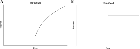
The two general shapes of a threshold effect are depicted in Figures 1a and 1b. Characteristic of a threshold effect is the absence of an effect for exposure doses below some “critical” threshold value coupled with a significant harmful effect for dosages greater than threshold; Cornfield (1977) calls this a hockey-stick effect. Hockey-stick effects on a continuous scale are of the type shown in Figure 1a; the effects on a yes/no or present/absent type scale are as in Figure 1b.

FIGURE 1.

Shapes of Threshold Effect Relationships Between Dose and Response. a, continuous response; b, binary response.

U- or J-shaped effect

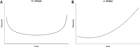
Nonlinear relationships that are U- or J-shaped are depicted in Figures 2a and b, respectively; illustrated are the characteristic phenomena of adverse health effects at low and/or high doses of exposure and a null or beneficial association in an intermediate dose range.

FIGURE 2.

Shapes of U- and J-Effects.

3. STATISTICAL APPROACHES TO MODELING NONLINEAR RELATIONSHIPS

A large body of literature and many textbooks provide excellent treatments of the development, assessment, and interpretation of statistical models generally (e.g. Hosmer and Lemeshow, 2000; Seber and Lee, 2003; Kleinbaum, Kupper, Muller and Nizam, 1998). Typically, the methodology begins with estimating a linear relationship which, upon assessment, is believed to yield some clues regarding the underlying true functional form that relates the two variables. In the setting of this report, where initial estimation of a linear relationship may be misleading when the correct model is a non-linear dose-response relationship, we suggest that initial data analyses should include techniques that are especially appropriate for the detection of non-linearities. A variety of graphical approaches and formal tests are available for this.

Ordinal Reparameterization of Exposure

This approach entails retaining for analysis an ordinal reparameterization of exposure, rather than the continuously measured value itself. Albeit with some loss of information necessarily, valuable insights are possible when the substitute ordinal variable permits a meaningful test of trend, or an insight as to the nature of the functional relationship between exposure and outcome, or both. In its implementation, the range of the observed dose is divided into mutually exclusive subgroups and, within each subgroup, a common value of exposure assigned (typically the average for that subgroup). Exposure subgroup definitions might be based on statistical considerations (e.g. quantiles) or subject matter considerations (e.g. no exposure at all versus below legal limit versus above legal limit). Apparent trend in outcome with increasing dose of exposure can be assessed using the Mantel extension test for trend (Clayton and Hills, 1993, Mantel, 1963). Alternatively, the exposure subgroups can be used to define indicator variables for inclusion in a multivariable model of outcome; a plot of the estimated coefficients permits an easy graphical assessment of the assumption of linearity. Thus, advantages of this technique are its simplicity and apparent “model free” framework. There are disadvantages, too, however (e.g. Lagakos, 1988; Zhao and Kolonel, 1992; Greenland, 1995a), including its potential sensitivity to the choice of exposure subgroups and a loss of power.

Polynomial and Fractional Polynomial Modeling of Exposure

A polynomial parameterization of exposure is a model-based approach to exploring nonlinearity. In this technique, each exposure value is re-expressed as a polynomial of degree greater than one (eg. quadratic, cubic, etc), yielding an estimated model with multiple predictors (ie – separate predictors for the linear, quadratic, etc terms respectively). An example is the modeling of age; age might be modeled quadratically so as to accommodate a nonlinear effect on outcome in older persons. Testing the departure from zero of the coefficients for the higher order powers of exposure is an assessment of the adequacy of the linear model representation. The principal advantage of the use of a polynomial reparameterization of the predictor is that it yields a single model of the overall relationship. Often, a disadvantage is that this will be a poor fit in selected exposure dose ranges, especially the highest and the lowest. Some improvement in fit is achieved by the use of fractional polynomials or splines.

Fractional polynomials, developed by Royston and Altman (1994), are an extension of a polynomial reparameterization of the predictor (in our case, exposure) that permits consideration of fractional powers and the combination of terms (see e.g. Hosmer and Lemeshow, 2000 for an introduction). As with a polynomial reparameterization, a fractional polynomial representation of the predictor is used to estimate a single overall relationship between predictor and outcome. The use of fractional powers and the combination of terms can substantially improve the fit. Nevertheless, it may not represent well changes in functional form, such as abrupt changes in risk or changes in functional form occurring at very low or very high exposure levels (e.g. threshold effects).

Splines

The use of splines in modeling predictor-outcome relationships is also an extension of the polynomial reparameterization approach. Here, separate polynomials of the predictor (here, exposure) are fit for each subgroup of the sample defined by interval values (e.g. quantiles) of the predictor variable. As before, the partitioning of the sample into exposure subgroups can be based on either subject matter or statistical considerations. An overall smooth curve is obtained by fitting polynomials to the subgroups of the predictor variable and connecting them at the boundaries. Often, cubic splines are available in statistical software, but quadratic splines have also been recommended (Greenland, 1995b). Due to the fact that the fit of higher order polynomials is often a misrepresentation for the lowest and highest exposure categories, linear functions are fit for those. In this case the splines are called restricted splines.

Non-parametric smoothing techniques

A graphical approach that is useful for exploring dose-response relationships is that of smoothing. This technique does not make any assumptions regarding the nature of the relationship nor the distribution of either dose or response variable; assumed only is that the relationship is continuous. A particularly useful non-parametric smoothing technique is lowess (for locally weighted regression) smoothing. For each value of the independent variable, one estimates a separate linear regression model for the data contained in a window around this value. Values closer to the center of the window are weighted more than values close to the edges of the window. The results are summarized as a set of local regression prediction values, one for each window; the plot of these values is what comprises a lowess curve. The degree of smoothness of the resulting graph depends on the width of the window. Lowess curves are especially useful when the association is suspected to be different from a straight line. More generally, the use of smoothing techniques is an excellent approach for exploring nonlinear dose response relationships at a univariate level. Unfortunately, their use in multivariate settings is limited.

4. FACTORS HINDERING DETECTION OF NON-LINEAR DOSE-RESPONSE RELATIONSHIPS

Inadequate sample size, insufficient range, and individual susceptibility pose unique challenges in the discovery of non-linear relationships in epidemiologic studies.

Sample size

Insufficient sample size is known to reduce the likelihood of detecting a true relationship through its effect on both type I and type II error, all other things being equal. In the non-linear relationship setting, insufficient sample size poses another challenge as well. Specifically, for the detection of a non-linearity, there must be a reasonable number of data points in the actual region of non-linearity. Thus, it is not enough to have a large overall sample size; there must also be adequate sample sizes in the regions of nonlinearity in particular. This requirement is more easily met in experimental studies, as the investigator can set by design the sample sizes at each of the dose levels of interest. Observational epidemiologic studies, however, are problematic in this regard. Sample size-dose combinations cannot be set by the investigator and, often, there exist only small sample sizes for dose levels that are either very low or very high (the very intervals where non-linearity might be anticipated). Another example is the setting of studies of occupational health. It is difficult to obtain exposure-outcome data for persons with a large number of years of cumulative exposure to a putative carcinogen if federal guidelines limit this exposure. In these and similar examples, when the available data is sparse in the regions of nonlinearity, the result will be wide confidence bands about the estimated model that are difficult to interpret.

Range of exposure

Our understanding that a fitted line is generalizable to the observed range of data only, has implications in the non-linear setting. Specifically, if the available exposure levels are only in the region of the “stick” portion of the J-shaped curve, then the estimated relationship will be presumed to be linear and any inference of non-linearity will be missed altogether. Similarly, a threshold effect will be missed altogether, depending on the available range of exposure.

Individual susceptibility

Despite extensive research, for most diseases, we do not know all of the factors that contribute to the occurrence of the disease. Among the statistical treatments of the unknown factors is the practice of handling these as noise. Sometimes, however, it is meaningful to conceptualize these as individual susceptibility.

Problematic is that individual susceptibilities might be both important and inestimable. In population based studies of a non-linear dose-response relationship in particular, it may not be meaningful to postulate a single threshold dose for an entire population (Lutz, 2000) as, more reasonably, individual susceptibilities might take the form of individual, distinct, threshold dose values. The result is that, when characterizing a dose-response relationship at the population level, depending on the direction and magnitudes of the variations in individual susceptibility, the latter is indistinguishable from noise. Thus, it is similarly possible that, in the case of an underlying threshold effect, depending on the direction and magnitude of these individual variations in susceptibility, a population based study may or may not reveal the existence of any (individual or otherwise) threshold effect at all.

5. MISSPECIFIED MODELS

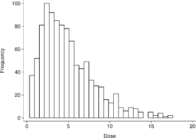
In the two settings that are of special interest here, those of threshold and U- or J-shaped effects, we illustrate the challenges and the limitations of a statistical analysis of a nonlinear dose-response relationship. Without loss of generality, we consider simulated data having a simple structure. Specifically, in both settings, noise is introduced by permitting individuals to have a different level of susceptibility. To keep things simple, noise is random. Data generation is also such that exposure dose is not uniformly distributed over the range of observed levels of dose. Instead, and in accordance with prevalence patterns that are likely to be encountered in epidemiologic studies, dose levels are generated such that the majority of the analytic sample has low or medium exposure values while the remaining minority have high levels of exposure. See Figure 3 for the distribution of dose levels used for both threshold and J-shaped settings.

FIGURE 3.

Distribution of Dose for threshold and J-effect scenarios

5.1. True dose-response relationship: Threshold

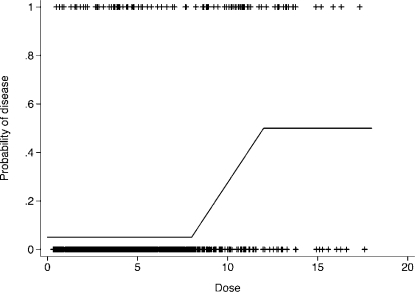
We generated a data set of size n = 1000 in which exposure dose levels range from 0 to 18 and the overall prevalence of disease is equal to 10%. Outcome status, defined as disease or non-disease, was generated such that disease has an expected relative frequency of 5% for dose levels below 8, then increases linearly from 5 to 50% for dose levels from 8 to 12, and is 50% for dose levels exceeding 12. See Appendix for details on the generation of these data. A graphical representation of the probability of disease occurrence and disease status for the generated example data is given in Figure 4.

FIGURE 4.

Probability of disease occurrence and disease status as generated for threshold model

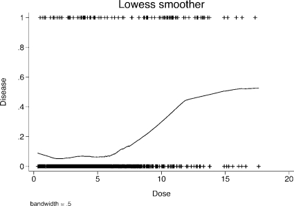
To illustrate the capabilities of smoothing techniques, following is a graph of the estimated probabilities of having the disease using the example data and a lowess smoother (Figure 5). As can be seen, the estimated form for the probability of having the disease does resemble the form which was used to generate the data.

FIGURE 5.

Lowess smoother of the probability of having the disease in the threshold example data

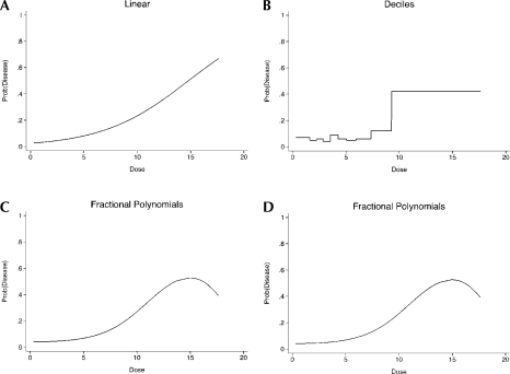
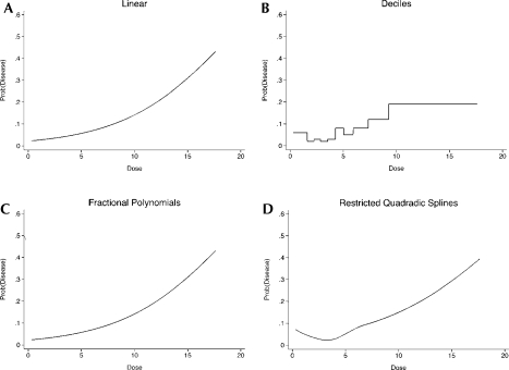
An analysis of the data naïve to the possibility that the relationship is threshold shaped might proceed with the following five results. (1) A logistic regression model is estimated assuming a linear relationship on the log odds scale. The odds of disease are estimated to increase by approximately 28% for each unit increase in dose (Figure 6). The associated significance level is a p-value less than 0.001. An assessment of goodness-of-fit for this model using the Hosmer-Lemeshow (2000) test suggests rejection of the null hypothesis of an adequate fit (p = 0.03). (2) Consideration of a polynomial representation on the logit scale, in particular quadratic in dose, is not a statistically significant improvement over the linear model (results not shown since they are almost identical to the linear fit). (3) We consider an ordinal reparameterization using deciles of dose and fitting dummy variables with the first group being the referent group (Figure 6). The odds of having the disease is only statistically significantly increased for the last decile (with a p-value of less than 0.001). If less than 10 groups are considered the results are very similar, in that the odds of having the disease is always statistically significant for the group including the highest levels of dose (results not shown). (4) Expansion of the possible functional forms to the family of fractional polynomials identifies as the best fitting model a sigmoidal shape with a drop at the highest level of dose (functional form: logit [disease] = dose³ + dose³(log(dose)), Figure 6); it is a statistically significant improvement over the linear model (p < 0.01). (5) Finally, consideration of a model comprised of quadratic splines for quartiles of dose suggests a sharp increase in the logit for higher levels of dose (Figure 6).

FIGURE 6.

Estimated probabilities for the threshold example for the following approaches of modeling dose: Linear, ordinal (deciles), fractional polynomials, and restricted quadratic splines

Comparison of the four panels in Figure 6 reveals that, in this example, the estimation of the ordinal representation, the fractional polynomial and quadratic spline models permits detection of a relatively sharp increase in odds of disease with higher levels of dose. A drawback to the estimated fractional polynomial model is that it suggests a drop in odds of disease for the highest levels of dose, in contrast to the relationship used to generate the data. The estimated quadratic splines model is misleading as well; notice the consistently increasing estimated risk for high levels of dose. This characteristic remains the same even if deciles of the exposure are used instead of quartiles (results not shown). We note also (results not shown) that consideration of unrestricted splines also suggests, mistakenly, that there is a drop in odds of disease for the highest levels of dose. Thus, while consideration of fractional polynomials and splines is an enhancement of logit models that are linear or polynomial, the former are difficult to interpret, particularly in the range of high values of the predictor variable (e.g. dose). That fractional polynomial and quadratic spline models are potentially instable in the tails, as has been noted by other authors as well (e.g. Greenland, 1995b). This has led to the recommendation to use restricted splines instead of unrestricted splines.

5.2. True dose-response relationship: J-shaped

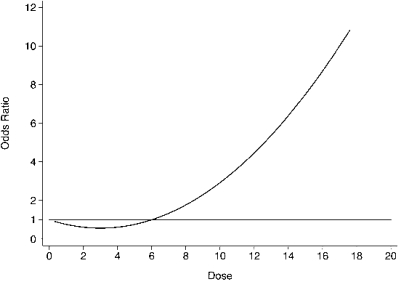
For this illustration, we generated 1000 outcomes (presence or absence of disease) such that estimated odds ratios relating exposure to logit[disease] follows a quadratic function. The overall prevalence of disease equals 7%. See Appendix for details on the generation of these data. A graphical representation of the odds ratio for disease occurrence is given in Figure 7.

FIGURE 7.

Relationship between odds ratios and dose for data generated to exhibit J-shaped effect

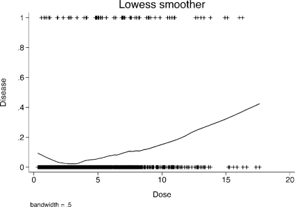
A graph of estimated probabilities of disease in the sample data using a lowess smoother is shown in Figure 8 and does resemble a J-shaped effect.

FIGURE 8.

Lowess smoother of the probability of having the disease in the J-effect example data

Analysis of these data naïve to the possibility of a J shaped relationship yields the following five results. (1) Based on the estimation of a logistic regression model that assumes linearity on the logit scale, the odds of disease is estimated to increase by approximately 22% for each unit increase in dose (Figure 9); the statistical significance of this finding is a p-value less than 0.001. The Hosmer-Lemeshow (2000) goodness-of-fit test fails to reject the hypothesis of an adequate fit (p = 0.39). (2) Expansion of the estimated model to include a quadratic effect in dose is not a statistically significant improvement (results not shown since they are again almost identical to the linear fit). (3) Considering an ordinal representation using deciles of dose and fitting dummy variables with the first being the referent group (Figure 9) yields estimated increases in odds of disease with each decile of exposure that is statistically significantly only for the last decile (with a p-value of less than 0.001). If less than 10 groups are considered the results are very similar with the following exception. When using 7 groups of dose, the odds of having the disease is borderline statistically significant for the second group compared to the first (referent) group (p-value = 0.07). (4) In this example, consideration of the family of fractional polynomials does produce a “best” fitting model that is J shaped (functional form: logit[disease] = log(dose) + (log(dose))², not shown). However, its improvement over the linear model is not statistically significant; thus, we might infer that a linear relationship is an adequate fit to the data (Figure 9). (5) Finally, the estimation of restricted quadratic splines for quartiles of dose reveals the general functional form as generated (Figure 9).

FIGURE 9.

Estimated probabilities for the J-effect example for the following approaches of modeling dose: Linear, ordinal (deciles), fractional polynomials, and restricted quadratic splines

A comparison of the four panels in Figure 9 shows that, in this example, only the quadratic spline model detects correctly the J-shaped relationship comprised of an initial drop in risk followed by a steady increase. The ordinal parameterization gives some indication, but not a statistically significant suggestion of a J-shaped relationship. Both the linear and fractional polynomial approaches are misleading; they fail to detect the protective effect at low dose levels.

6. DISCUSSION

Our two simulations of threshold and J-shaped relationships were designed to be simplified, but reasonable representations of real world data having critical characteristics typically encountered in epidemiologic data: (1) the distribution of the exposure variable is not uniform and (2) there is variability in the individual responses which might be characterized as individual susceptibility. We have applied several straightforward statistical approaches to analyze the relationships. The finding that the methodologies we employed were inconsistent in the detection of the underlying relationships is important. Specifically, “straightforward statistical approaches” may fail us in the non-linear setting.

Note that an illustration of U-shaped dose-response data would reveal that an initial linear fit would typically fail to detect the non-linear shape altogether. This is the case, since in U-shaped dose response relationships elevated risks at low and high exposure levels would “cancel out” more protective effects at intermediate levels

Our illustrations reveal multiple advantages and caveats of using ordinal, polynomial, and spline parameterizations of exposure in the setting of threshold or J effect relationships. Principal among the advantages is that the general shape of the dose-response relationship can be inferred. Thus, we recommend against initial treatments of data that are limited to the fit of a linear approximation. We also recommend against any other single approach, especially as there exists statistical software that make it straightforward to consider several approaches like ordinal, polynomial and spline reparameterizations of the predictor variable.

The caveats are especially noteworthy for their insights to choice of analysis. In the threshold effect setting, both fractional polynomial and spline parameterizations of exposures were partly misleading; the former suggested a drop in risk for the highest levels of exposure and the latter suggested a consistent increase in risk for higher levels of exposure.

With respect to U and J-shaped effect relationships, there exist formal statistical tests for assessing whether an enlarged model (e.g. fractional polynomial or restricted splines) represents an improvement over a linear relationship. To our knowledge, however, there do not exist such tests for threshold effect relationships which can be used in epidemiological investigations. There exists only a test of this type for use in experimental settings (Lutz et al., 2002). The development of a test for a threshold effect for non-experimental settings would be desirable, but might be either impossible or of limited practical value given the specific challenges of observational data.

Various authors have commented on the significant limitations of the use of categorical variables to assess the effect of a continuous exposure (e.g. false precision and loss of information). The advantages of the use of fractional polynomials and splines have also been pointed out (e.g. consideration of a larger family of possible functional form). We do not disagree with either of these assessments. However, we view the use of categorical variables for purposes of exploration as potentially yielding important insights. For example, in epidemiological investigations, if the underlying dose-response relationship represents a threshold effect, the use of categories has the potential to provide more clear insights to this relationship than either fractional polynomials or splines.

We reason that, provided they are examined collectively, each of several approaches (ordinal reparameterization, fractional polynomials, splines, etc) can contribute meaningfully to the discovery of a nonlinear dose-response relationship. Thus, we recommend using multiple approaches when exploring the possibility of a nonlinear dose response relationship. The caveat to this recommendation is that the results from each of the approaches should be judged in the context of its specific limitations.

APPENDIX

Non-linear models

We wish to clarify a distinction that is relevant to this report, that between “non-linear relationship” and “non-linear statistical model”. “Non-linear relationships” are true non-linear phenomena. Threshold effects, U-shaped effects, selected laws of physics (like the exponential decay model) are examples. In contrast, a statistical model that is non-linear in the independent variables (for example, modeling the effect of age as a quadratic effect) is nevertheless “statistically” linear when it is linear in the estimated parameters. Thus, like statistical interactions, statistical linearity refers to choice of scale, not nature.

Currently, theoretically based formulas are typically not available for epidemiologic investigations of non-linear phenomena. In the absence of such theory, in most cases, statistically linear models which include non-linear modeling of the independent variables represent an adequate approximation of the relationship of interest. Thus, the focus in this report has been on models that are linear in the parameters but are non-linear in the independent variables. Accordingly, the use of the term “nonlinear” in this article refers to the relationship, not the statistical model.

Data generating procedures

For both, the threshold and the J-shaped example 1000 observations were generated randomly, such that the exposure variable dose follows a chi-square distribution with an expected value of 5 (see Figure 3 for the distribution of dose).

For the threshold example, the outcome (absence or presence of disease) was generated such that (uniformly) 5% of the observations with dose levels below 8 and (uniformly) 50% of the observations with dose levels above 12 exhibit the disease. For dose levels between 8 and 12, disease status was generated such that the probability of having the disease increases linearly from 5 to 50%.

For the J-shaped example, the outcome (absence or presence of disease) was generated such that the relative risk of disease represents a quadratic function of the exposure (dose). Specifically, the functional form for the relative risk was generated as 1 – 54/187 dose + 9/87 dose². This form was chosen such that a dose of level 0 and 6 result in a relative risk of 1, and a dose of level 17 results in a relative risk of 10. Using the quadratic form, a relative risk was determined for each observation. Using the logistic model, the probability of having the disease was specified according to the assigned relative risk while assuming a background prevalence of the disease of 5% (Prob = [1/(1_exp(–1∗(–2.944 + log(Relative Risk))))]). The generated probabilities were subsequently used to randomly assign the disease status for each of the observations.

REFERENCES

- Becher H. Analysis of continuous covariables in epidemiological studies: Dose-response modeling and confounder adjustment. Biometrical Journal. 2002;44(6):683–699. [Google Scholar]
- Boucher KM, Slattery ML, Berry TD, et al. Statistical methods in epidemiology: A comparison of statistical methods to analyze dose-response and trend analysis in epidemiologic studies. Journal of Clinical Epidemiology. 1998;51(12):1223–1233. doi: 10.1016/s0895-4356(98)00129-2. [DOI] [PubMed] [Google Scholar]
- Clayton D, Hills M. Statistical Models in Epidemiology. New York: Oxford; 1993. [Google Scholar]
- Cornfield J. Carcinogenic risk assessment. Science. 1977;198(4318):693–699. doi: 10.1126/science.910152. [DOI] [PubMed] [Google Scholar]
- D'Agostino R.B., Belanger A.J., Kannel W.B., Higgins M. Role of smoking in the U-shaped relation of cholesterol to mortality in men. The Framingham study. Am J Epidemiol. 1995;141:822–827. doi: 10.1093/oxfordjournals.aje.a117517. [DOI] [PubMed] [Google Scholar]
- De Flora S. Threshold mechanisms and site specificity in chromium(VI) carcinogenesis. Carcinogenesis. 2000;21:533–541. doi: 10.1093/carcin/21.4.533. [DOI] [PubMed] [Google Scholar]
- Greenland S. Avoiding Power loss associated with categorization and ordinal scores in Dose-Response and Trend analysis. Epidemiology. 1995;6:450–454. doi: 10.1097/00001648-199507000-00025. [DOI] [PubMed] [Google Scholar]
- Greenland S. Dose-response and trend analysis in epidemiology –Alternative to categorical analysis. Epidemiology. 1995;6(4):356–365. doi: 10.1097/00001648-199507000-00005. [DOI] [PubMed] [Google Scholar]
- Hannson L. Treatment of hypertension and the J curve. Journal of Hypertension. 1999;1(2):136–140. [PubMed] [Google Scholar]
- Hosmer DW, Lemeshow S. Applied Logistic Regression. New York: Wiley; 2000. [Google Scholar]
- Jones R.E. Hexavalent chrome: threshold concept for carcinogenicity. Biomed Environ Sci. 1990;3:20–34. [PubMed] [Google Scholar]
- Kleinbaum DG, Kupper LL, Muller KE, Nizam A. Applied Regression Analysis and Other Multivariable Methods. Pacific Grove: Duxbury Press; 1998. [Google Scholar]
- Lagakos SW. Effects of mismodeling and mismeasuring explanatory variables on tests of their association with a response variable. Statistics in Medicine. 1988;7:257–274. doi: 10.1002/sim.4780070126. [DOI] [PubMed] [Google Scholar]
- Mantel N. Chi-square tests with one degree of freedom: extensions of the Mantel-Haenszel procedure. Journal of the American Statistical Association. 1963;58:690–700. [Google Scholar]
- Mundt K.A., May S. Epidemiological Assessment of Hormesis. Human and Ecological Risk Assessment. 2001;7:795–809. [Google Scholar]
- Lamm SH, Walters AS, Wilson R, Byrd DM, Grunwald H. Consistencies and inconsistencies underlying the quantitative assessment of leukemia risk from benzene exposure. Environ Health Perspect. 1989;82:289–97. doi: 10.1289/ehp.8982289. Review. [DOI] [PMC free article] [PubMed] [Google Scholar]
- Littlefield NA, Farmer JH, Gaylor DW, Sheldon WG. Effects of dose and time in a long-term, low-dose carcinogenic study. J Environ Pathol Toxicol. 1980;3:17–34. [PubMed] [Google Scholar]
- Luippold R.S., Mundt K.A., Austin R.P., Liebig E., Panko J., Crump C., Crump K., Protor D. Lung cancer mortality among chromate production workers. Occup Environ Med. 2003;60:451–457. doi: 10.1136/oem.60.6.451. [DOI] [PMC free article] [PubMed] [Google Scholar]
- Lutz WK. A true threshold dose in chemical carcinogenesis cannot be defined for a population, irrespective of the mode of action. Hum Exp Toxicol. 2000;19(10):566–8. doi: 10.1191/096032700701546488. discussion 571–2. [DOI] [PubMed] [Google Scholar]
- Lutz RW, Stahel WA, Lutz WK. Statistical procedures to test for linearity and estimate threshold doses for tumor induction with nonlinear dose-response relationships in bioassays for carcinogenicity. Regul Toxicol Pharmacol. 2002;36(3):331–7. doi: 10.1006/rtph.2002.1583. [DOI] [PubMed] [Google Scholar]
- Lutz WK, Vamvakas S, Kopp-Schneider A, Schlatter J, Stopper H. Deviation from additivity in mixture toxicity: relevance of nonlinear dose-response relationships and cell line differences in genotoxicity assays with combinations of chemical mutagens and gamma-radiation. Environ Health Perspect 110 Suppl. 2002;6:915–8. doi: 10.1289/ehp.02110s6915. [DOI] [PMC free article] [PubMed] [Google Scholar]
- Perry IJ, Wannamethee SG, Whincup PH, Shaper AG, Walker MK, Alberti KG. Serum insulin and incident coronary heart disease in middle-aged British men. Am J Epidemiol. 1996;144(3):224–34. doi: 10.1093/oxfordjournals.aje.a008917. [DOI] [PubMed] [Google Scholar]
- Ritz E, Koch M. Morbidity and mortality due to hypertension in patients with renal failure. Am J Kidney Dis. 1993;1:113–8. doi: 10.1016/0272-6386(93)70102-5. [DOI] [PubMed] [Google Scholar]
- Rothkamm K, Lobrick M. Evidence for a lack of DNA double-strand break repair in human cells exposed to very low x-ray doses. Proceedings of the National Academy of Science. 2003;100(9):5057–5062. doi: 10.1073/pnas.0830918100. [DOI] [PMC free article] [PubMed] [Google Scholar]
- Rothman KJ, Cann CI, Flanders D, Fried MP. Epidemiology of laryngeal cancer. Epidemiol Rev. 1980;2:195–209. doi: 10.1093/oxfordjournals.epirev.a036223. [DOI] [PubMed] [Google Scholar]
- Royston P, Altman DG. Regression using fractional polynomials of continuous covariates: Parsimonious parametric modeling (with discussion) Applied Statistics. 1994;43:429–467. [Google Scholar]
- Seber GAF, Lee AJ. Linear Regression Analysis. New Jersey: Wiley; 2003. [Google Scholar]
- Smith RL, Spitzner D, Kim Y, Fuentes M. Threshold dependence of mortality effects for fine and coarse particles in Phoenix, Arizona. J Air Waste Manag Assoc. 2000;50(8):1367–79. doi: 10.1080/10473289.2000.10464172. [DOI] [PubMed] [Google Scholar]
- Sommer A. Uses and misuses of vitamin A. Current Issues in Public Health. 1996;2(4):161–164. [PubMed] [Google Scholar]
- Zhao LP, Kolonel LN. Efficiency loss from categorizing quantitative exposures into qualitative exposures in case-control studies. American Journal of Epidemiology. 1992;163:464–474. doi: 10.1093/oxfordjournals.aje.a116520. [DOI] [PubMed] [Google Scholar]