The Effect of Random Error in Exposure Measurement upon the Shape of the Exposure Response

Abstract

Although statistical analyses of epidemiological data usually treat the exposure variable as being known without error, estimated exposures in epidemiological studies often involve considerable uncertainty. This paper investigates the theoretical effect of random errors in exposure measurement upon the observed shape of the exposure response. The model utilized assumes that true exposures are log-normally distributed, and multiplicative measurement errors are also log-normally distributed and independent of the true exposures. Under these conditions it is shown that whenever the true exposure response is proportional to exposure to a power r, the observed exposure response is proportional to exposure to a power K, where K < r. This implies that the observed exposure response exaggerates risk, and by arbitrarily large amounts, at sufficiently small exposures. It also follows that a truly linear exposure response will appear to be supra-linear—i.e., a linear function of exposure raised to the K-th power, where K is less than 1.0. These conclusions hold generally under the stated log-normal assumptions whenever there is any amount of measurement error, including, in particular, when the measurement error is unbiased either in the natural or log scales. Equations are provided that express the observed exposure response in terms of the parameters of the underlying log-normal distribution. A limited investigation suggests that these conclusions do not depend upon the log-normal assumptions, but hold more widely. Because of this problem, in addition to other problems in exposure measurement, shapes of exposure responses derived empirically from epidemiological data should be treated very cautiously. In particular, one should be cautious in concluding that the true exposure response is supra-linear on the basis of an observed supra-linear form.

INTRODUCTION

Statistical analyses of epidemiological data usually treat the exposure variable as being known without error. However, in many studies the exposure measure is very uncertain, perhaps more so than that of the health endpoint serving as the dependent variable. Research into the effect of exposure measurement error has focused primarily on its effect upon the ability to detect exposure responses and to correct biases in regression slopes (see e.g., Thomas et al. 1993); less attention has been directed at understanding the effect of exposure error upon the shape of the exposure response.

Herein, the primary concern regarding the “shape of the exposure response” is whether the increase in health outcome with increasing exposure is linear when plotted against exposure, supra-linear (a steeper increase in response with increasing exposure at lower exposures than at higher exposures, as represented by exposure to the K-th power, with K <1), or sub-linear (a less steep increase in response at lower exposures than at higher exposures, as represented by exposure to the K-th power, with K >1). A threshold response, in which there is no effect of exposure until an exposure threshold is exceeded, can be thought of as a special case of a sub-linear response.

Exposure-response analyses of epidemiological data are sometimes used to predict risks at exposure levels that are below those at which risks can reliably be measured directly. If the exposure-response from an epidemiological study is used for this purpose, then the shape of the exposure response will be a critical determinant of the resulting risk levels. In addition, some guidelines for setting health standards (e.g., USEPA 2003) mandate radically different approaches for setting exposure standards in cases where the exposure response is “non-linear” (specifically, sub-linear), as opposed to cases in which the exposure response is linear. If the shape of the exposure response from an epidemiological study is used to decide between “linear” and “non-linear”, the observed shape of the exposure response curve will be important in setting exposure standards.

In this note we point out that even unbiased errors in exposure can cause systematic distortion of the shape of the exposure response. In particular, such errors tend to cause risks from low exposures to be exaggerated and to make a linear exposure response appear supra-linear.

METHODS AND RESULTS

For illustrative purposes we consider the case of a power function exposure response (i.e., we assume the exposure-related increase in the expected health outcome is proportional to the r-th power of the true exposure) and investigate the effect of exposure error upon this exposure response. Let O represent the health outcome of a person randomly selected from an exposed population, and let D_T and D_M represent his true and measured exposures, respectively. We assume that O, D_T and D_M are random variables. The assumed (true) exposure response can be expressed mathematically as

$$\text{E}(\text{O}|{\text{D}}_{\text{T}})=\alpha +\beta \ast {\text{D}}_{\text{T}}^{\text{r}},$$

for some constants α and β, where the left-hand side of this equation denotes the conditional expectation of the health outcome, O, given the true exposure D_T. A linear exposure response corresponds to the special case r = 1.

The observed exposure response is represented by E(O | D_M), the expected value of the health outcome given the measured value. To compute this quantity we need to assume that E(O | D_T, D_M) = E(O | D_T), i.e., that once the true exposure is known, the measured exposure provides no additional information on the value of the health outcome. With this assumption, and using basic properties of conditional expectation, if follows that

$$\begin{array}{cc}\text{E}(\text{O}|{\text{D}}_{\text{M}})& =\text{E}(\text{E}(\text{O}|{\text{D}}_{\text{T}},{\text{D}}_{\text{M}})|{\text{D}}_{\text{M}})\\ & =\text{E}(\text{E}(\text{O}|{\text{D}}_{\text{T}})|{\text{D}}_{\text{M}})\\ & =\text{E}(\alpha +\beta \ast {\text{D}}_{\text{T}}^{\text{r}}|{\text{D}}_{\text{M}})\\ & =\alpha +\beta \ast \text{E}({\text{D}}_{\text{T}}^{\text{r}}|{\text{D}}_{\text{M}})\end{array}$$ (1)

Thus, the observed exposure response is a linear function of the conditional expectation of the true exposure, raised to the r-th power, given the measured exposure.

To proceed, assumptions are needed regarding the distributions of D_T and D_M. We assume that D_T is log-normally distributed, with Ln(D_T) having mean μ and standard deviation σ. The expected value of D_T is (Johnson et al. 1994)

$$\text{E}({\text{D}}_{\text{T}})=exp(\mu +{\sigma }^2/2).$$ (2)

We further assume that the measured exposure can be expressed as the product of the true exposure and a multiplicative measurement error, i.e., D_M = D_T ∗ D_E, where the multiplicative error, D_E, is independent of the true exposure, D_T, and also has a log-normal distribution. The mean of Ln(D_E) will be denoted by γ and its standard deviation by τ. Under these conditions, the measured exposure D_M also has a log-normal distribution, with expected value given by

$$\text{E}({\text{D}}_{\text{M}})=exp(\mu +{\sigma }^2/2+\gamma +{\tau }^2/2)$$ (3)

For the mean of a sample of observed exposures, D_M, to be an unbiased estimate of the true mean exposure requires that E(D_E) = 1, which is true if and only if γ = –τ²/2. Similarly, Ln(D_M) is an unbiased estimate of the mean of the log-transformed exposures if and only if γ = 0.

Conditional on the measured value, D_M = d, D_T can be shown (using properties of the bivariate normal distribution; see, e.g., Mood and Graybill 1963) to have a log-normal distribution with the logarithm of the true exposure having conditional expected value

$$\text{E}[\text{Ln}({\text{D}}_{\text{T}})|{\text{D}}_{\text{M}}=\text{d}]=\{\mu \ast {\tau }^2+{\sigma }^2\ast [\text{Ln}(\text{d})-\gamma ]\}/({\sigma }^2+{\tau }^2),$$ (4)

and conditional variance

$$\text{Var}[\text{Ln}({\text{D}}_{\text{T}})|{\text{D}}_{\text{M}}=\text{d}]={\sigma }^2\ast {\tau }^2/({\sigma }^2+{\tau }^2).$$ (5)

Using the formulas for the expectation of the r-th power of a log-normal distribution in terms of the mean and variance of the log-transformed variate (equation 1) it follows that, conditional on the measured value, the expected value of the true exposure raised to the r-th power conditional on the measured value, D_M = d, is (Johnson et al. 1994),

$$\text{E}({\text{D}}_{\text{T}}^{\text{r}}|{\text{D}}_{\text{M}}=\text{d})=\text{A}\ast {\text{d}}^{\text{K}},$$ (6)

where the constant multiplier A is given by

$$\text{A}=exp\left\{[\text{r}\ast \mu \ast {\tau }^2+\text{r}\ast {\sigma }^2\ast (\text{r}\ast {\tau }^2/2-\gamma )]/({\sigma }^2+{\tau }^2)\right\},$$ (7)

and the exponent K by

$$\text{K}=\text{r}\ast {\sigma }^2/[{\sigma }^2+{\tau }^2].$$ (8)

Consequently, from expression (1), the observed exposure response is given by

$$\text{E}(\text{O}|{\text{D}}_{\text{M}}=\text{d})=\alpha +\beta \ast \text{A}\ast {\text{d}}^{\text{K}}.$$ (9)

It is important to note that, unless there is no measurement error (τ = 0), the exponent K is less than r. Thus, in this case, measurement error will always cause the exponent in the exposure response to shift in the direction of from sub-linear to supra-linear. E.g., a linear exposure response (r = 1) will appear supra-linear (K < 1). The degree of shift from sub-linearity to supra-linearity (i.e., the amount by which K is less than r) depends upon the relative size of the variance, τ², of the multiplicative errors, D_E, in comparison to the variance, σ², of the true exposures, D_T. For example, if the true exposure response is quadratic (r = 2), but the measurement error variance exceeds the variance of the true exposure distribution (τ² > σ²) then K < 1, and the observed exposure response will be supra-linear. It should also be noted that, since d^K/d^r tends towards infinity as d tends towards zero, the observed exposure response will always overestimate the true exposure response by arbitrarily large factors at sufficiently small exposures, irrespective of the true exposure response (value of r).

The range of exposures over which the observed exposure response overestimates the true response is composed of those exposures, d, for which A ∗ d^K > d^r. Solving this expression for d leads to the conclusion that the observed exposure response overestimates the true exposure response for exposures, d, such that

$$\text{d}<exp[\mu +{\sigma }^2\ast (\text{r}/2-\gamma /{\tau }^2)],$$ (10)

and underestimates responses for larger values of exposure. In the special case of a linear exposure response (r = 1) and measured exposures are unbiased (γ = –τ²/2), the observed exposure response is an overestimate whenever the true exposure is less than exp(μ + σ²), the probability of this occurrence being N(σ) = N{[ln(1 + c²)]^0.5}, where c is the coefficient of variation of the log-normal distribution, and N() is the standard normal distribution. This expression is always greater than 0.5, and, for example, if c = 1, then the probability is 0.8. In the special case of a linear exposure response and γ = 0 (corresponding to the measured exposures being unbiased on a log scale), the right side of expression (10) reduces to the mean of the true exposure.

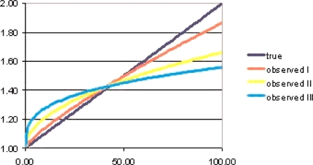
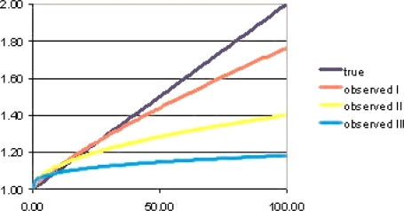
Figures 1 and 2 contain graphs comparing the true and observed exposure responses for various cases. In both figures the true response increases linearly (r = 1) from 1 to 2 as exposure increases from 0 to 100, and σ is fixed at σ = 1. Three values of τ are considered (τ = 0.5, 1, 1.5) corresponding to different amounts of exposure error in relation to the spread in the true exposures. With each value of τ selected, μ is chosen so that 95% of the measured exposures are less than 100, the maximum exposure graphed.

FIGURE 1.

True and observed dose responses, measured exposures unbiased (γ = –τ²/2)

FIGURE 2.

True and observed dose responses, measured exposures unbiased on a log scale (γ = 0)

Figure 1 considers the case in which measurement errors are unbiased (γ = –τ²/2). As this figure indicates, large exposure errors, even if they are unbiased, can lead to extreme distortion of the exposures response. E.g., with τ = 1.5, the observed exposure response rises almost vertically from 1 to 1.2 and then flattens out, approaching horizontal. The flattening is less severe with smaller values of τ (1.0 and 0.5). However, it should be kept in mind that all three observed exposures responses overestimate the true increase over the background value of 1 by arbitrarily large factors for very small exposures. In all three cases, the observed exposure response overestimates the true one for exposures below the exposure value of about 50 and underestimates for higher exposures.

Figure 2 was constructed in a manner identical to Figure 1 except it considers the case in which measured exposures are unbiased on a log scale (γ = 0). Here the range of exposures for which overestimation occurs is narrower, but the degree of underestimation at the highest exposures is more severe.

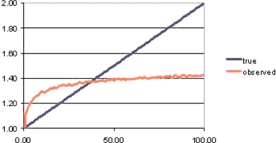
All the results presented thus far assume a log-normal for both true exposures and exposure errors. Other distributional assumptions are more difficult to investigate because the distribution of the true exposures conditional on the measured exposures is generally not mathematically tractable. To give some indication of the robustness of the results reported herein to the log-normal assumption, one calculation was made assuming a uniform distribution of true exposures (uniform between 0 and 110), with independent log-normally distributed error (γ = 0, τ = 1.3). The corresponding observed exposure response, computed using Markov Chain Monte Carlo (Gilks et al. 1996), is shown in Figure 3. This observed response is very similar in shape to those shown in Figures 1 and 2, which shows that the assumptions of log-normality are not necessary for our general conclusions.

FIGURE 3.

True and observed responses assuming true exposures are uniformly distributed

DISCUSSION

This work demonstrates that measurement errors, even if unbiased, distort the shape of the exposure response curve. In the situations considered herein, that distortion always converts an exposure response in the direction of from sub-linearity to supra-linearity; e.g., a linear exposure response is converted into a supra-linear shape. Although the analysis did not define the range of circumstances under with this type of distortion occurs, it did confirm that it always occurs with log-normally distributed exposures and independent log-normally distributed errors. This formulation should be general enough to approximate a wide range of conditions involving random, independent exposure errors. A qualitatively very similar result was obtained assuming a uniform distribution of true exposures (Figure 3). Thus, the effect of random exposure error seems to be in the direction of making low exposures appear more dangerous than they actually are.

The results derived herein apply to the theoretical (i.e., expected) response. The effect of random error in the dependent variable was not investigated. Except for assuming a specific form for the expected value of the response variable given the true exposure, no other assumption was made about the form of the response variable. Consequently, these results apply equally to continuous and categorical responses.

Thus, it is reasonable to conclude that random independent exposure errors in general tend to convert exposure responses in the direction of from sub-linearity to supra-linearity. A threshold response is a special case of sub-linearity, in which case random errors would obscure the threshold by improperly assigning exposure-related cases occurring above the exposure threshold to lower exposures, and thereby making a sub-linear exposure response appear more linear.

The underlying model of measurement errors used herein will generally be an oversimplification the true situation. For example, the assumption of independence of true exposures and measurement errors may not be warranted. In occupational cohort studies exposures are often assigned to work areas based on often limited sampling, perhaps supplemented with ad hoc information, and then linked to individual workers through work histories. In this situation, exposure errors of workers that worked in the same location would not be independent. Exposure errors in different locations could also be different. Although such potential problems suggest that the analysis provided herein is oversimplified, their existence does not suggest that the problem of the distortion of the exposure response is overstated, but rather provide even more evidence that the observed exposure-response shape may be unreliable.

The degree of distortion of the exposure response depends upon the spread of the measurement error distribution (τ) in comparison to the spread of the true exposure distribution (σ). In practice this is a very difficult issue to investigate. Thomas et al. (1993) discuss several methods of dealing with measurement error when analyzing epidemiology data, none of which are very satisfactory. The most general method is the “full likelihood” method in which assumptions are made regarding the joint distribution of true exposures, measurement errors, and the true exposure response, and the resulting likelihood of the observed data (both measured exposures and health outcomes) is calculated. Since the true exposures cannot be observed, the specification of their distribution will be very uncertain. The computation of the likelihood will be computationally complex since even with lognormal assumptions, the unknown true exposures will have to be integrated out of the likelihood using numerical integration. It seems unlikely that this approach would provide definitive information on whether the assumed exposure response is valid.

In addition to random exposure errors, there are other sources of distortion of the shape of the exposure response. If a study utilizes an inappropriate control group in which the response is low compared to that expected in the study population, the exposure response will tend toward an appearance of supra-linearity. Systematic errors in exposure also clearly can distort the shape of the exposure response. One example of this is when the highest exposures are overestimated by not modifying results from area samples to account for the use of respirators.

Because of these potential distortions of the exposure response shape, one should be cautious in drawing conclusions about the shape of the exposure response from epidemiological data. Since even random, unbiased errors in exposure measurement will convert a linear exposure response, and can a convert sub-linear response, into a seemingly supra-linear shape, one should be particular cautious about concluding an exposure-response is truly supra-linear. In particular, it could be inadvisable to extrapolate an observed supra-linear exposure response to low exposures to predict human risk.

REFERENCES

- Gilks WR, Richardson S, Spiegelhalter DJ. Markov Chain Monte Carlo in Practice. Boca Raton: Chapman & Hall/CRC; 1996. Introducing Markov chain Monte Carlo. [Google Scholar]
- Johnson NL, Kotz S, Balakrishnan N. Continuous Univariate Distributions. Second Edition. Volume 1. New York: John Wiley & Sons, Inc.; 1994. [Google Scholar]
- Mood AM, Graybill FA. Introduction to the Theory of Statistics. Second Edition. New York: McGraw-Hill Book Company, Inc.; 1963. [Google Scholar]
- Thomas D, Stram D, Dwyer J. Exposure measurement error: Influence on exposure-disease relationships and methods of correction. Annual Review of Public Health. 1993;14:69–93. doi: 10.1146/annurev.pu.14.050193.000441. [DOI] [PubMed] [Google Scholar]
- U.S. EPA. (2003) Draft Final Guidelines for Carcinogen Risk Assessment. Risk Assessment Forum, U.S. Environmental Protection Agency, Washington, DC. EPA/630/P-03/001A, NCEA-F-0644A.