Human ocular following initiated by competing image motions: evidence for a winner-take-all mechanism

B M Sheliga; Y Kodaka; E J FitzGibbon; F A Miles

doi:10.1016/j.visres.2005.11.033

. Author manuscript; available in PMC: 2008 Jul 23.

Published in final edited form as: Vision Res. 2006 Feb 20;46(13):2041–2060. doi: 10.1016/j.visres.2005.11.033

Human ocular following initiated by competing image motions: evidence for a winner-take-all mechanism

B M Sheliga ¹, Y Kodaka ¹, E J FitzGibbon ¹, F A Miles ¹

PMCID: PMC2481408 NIHMSID: NIHMS51211 PMID: 16487988

Abstract

The initial ocular following responses (OFRs) elicited by ¼-wavelength steps applied to the missing fundamental (mf) stimulus are in the backward direction and largely determined by the principal Fourier component, the 3^rd harmonic [Sheliga, Chen, FitzGibbon & Miles (2005) Initial ocular following in humans: A response to first-order motion energy. Vision Research, 45, 3307–3321]. When the contrast of the 3^rd harmonic was selectively reduced below that of the next most prominent harmonic—the 5^th, which moves in the opposite (forward) direction—then the OFR reversed direction and the 3^rd harmonic effectively lost all of its influence as the OFR was now largely determined by the 5^th harmonic. Restricting the stimulus to just two sine waves (of equal efficacy when of equal contrast and presented singly) with the spatial frequencies of the 3^rd and 5^th harmonics of the mf stimulus indicated that the critical factor was the ratio of their two contrasts: when of similar contrast both were effective (vector sum/averaging), but when the contrast of one was <½ that of the other then the one with the lower contrast became ineffective (winner-take-all). This nonlinear dependence on the contrast ratio was attributed to mutual inhibition and was well described by a weighted-average model with just two free parameters. Further experiments with broadband and dual-grating stimuli indicated that nonlinear interactions occur not only in the neural processing of stimuli moving in opposite directions but also of stimuli that share the same direction and differ only in their spatial frequency and speed. Clearly, broad-band and dual-grating stimuli can uncover significant nonlinearities in visual information processing that are not evident with single sine-wave stimuli.

Keywords: visual motion, energy-based mechanisms, missing fundamental, spatio-temporal filtering

1. Introduction

Ocular following responses (OFRs) are the machine-like tracking eye movements that can be elicited at ultra-short latency by sudden motion of a large textured pattern (Gellman, Carl & Miles, 1990; Miles, Kawano & Optican, 1986). Recent findings suggest that the very earliest OFR are mediated by motion detectors that are sensitive to 1^st-order motion energy, as in the well-known energy model of motion analysis (Adelson & Bergen, 1985; van Santen & Sperling, 1985; Watson & Ahumada, 1985). Thus, OFRs show clear reversal with “1^st-order reverse-phi motion”, one of the hallmarks of an energy-based mechanism (Masson, Yang & Miles, 2002a), and are very sensitive to the Fourier composition of the luminance modulations in the motion stimulus (Sheliga, Chen, FitzGibbon & Miles, 2005). The visual stimuli in this last study consisted of vertical square-wave gratings lacking the fundamental—referred to as the missing fundamental (mf) stimulus—and motion was applied in discrete ¼-wavelength steps. The OFRs associated with this motion stimulus were always reversed, i.e., rightward steps resulted in leftward OFRs. In fact it had been known for some time that the perceived direction of motion was often reversed when ¼-wavelength steps were applied to the mf stimulus (Adelson, 1982; Adelson & Bergen, 1985; Baro & Levinson, 1988; Brown & He, 2000; Georgeson & Harris, 1990; Georgeson & Shackleton, 1989). The explanation advanced for this apparent reversal of the OFR and perceived motion is that the underlying motion detectors do not sense the motion of the raw images (or their features) but rather a spatially filtered version of the images, so that the perceived motion depends critically on the Fourier composition of the spatial stimulus. In the frequency domain, a pure square wave is composed entirely of the odd harmonics (1^st, 3^rd, 5^th, 7^th etc.,) with progressively decreasing amplitudes such that the amplitude of the ith harmonic is proportional to 1/i. Accordingly, the mf stimulus lacks the 1^st harmonic and so is composed entirely of the higher odd harmonics, with the 3^rd having the lowest spatial frequency and the largest amplitude. This means that when the mf stimulus shifts ¼ of its (fundamental) wavelength, the largest Fourier component, the 3^rd harmonic, shifts ¾ of its wavelength in the same (forward) direction. However, a ¾-wavelength forward shift of a sine wave is exactly equivalent to a ¼-wavelength backward shift and, because the brain gives greatest weight to the nearest image matches (spatial aliasing), the OFR and seen motion are in the backward direction: see Fig. 1A–C. In fact, when ¼-wavelength steps are applied to the mf stimulus, all of the 4n-1 harmonics (where n is an integer), such as the 3^rd, 7^th, 11^th etc., will shift ¼ of their wavelength in the backward direction whereas all of the 4n+1 harmonics, such as the 5^th, 9^th, 13^th etc., will shift ¼ of their wavelength in the forward direction. Of course, each of the harmonics has a different apparent speed because the higher the spatial frequency the smaller the absolute magnitude of the shifts. In fact, the speed of the ith harmonic is proportional to 1/i. However, the most prominent harmonic in the mf stimulus—the 3^rd—generally dominates the perceived motion and the initial OFR. Thus, despite the broadband composition of the mf stimulus, with some harmonics moving in the forward direction, others moving in the backward direction, and all at different speeds, coherent motion is generally perceived (Georgeson & Shackleton, 1989). Further, the OFR associated with the mf stimulus often closely approximates the OFR elicited by the same steps applied to a pure sine wave whose spatial frequency and contrast match those of the 3^rd harmonic of the mf stimulus (Sheliga et al., 2005).

Fig. 1 — The mf and *mf-5* stimuli. Traces show luminance as a function of horizontal spatial position when the stimuli undergo successive ¼-wavelength *right*ward shifts. A–C: The mf stimulus; open circles and associated arrows indicate the *right*ward shifts of one particular peak in the profile (black in A and grey in B, C); black lines and associated arrows indicate the ¼-wavelength *left*ward shifts of the 3^rd harmonic (B) and the ¼-wavelength *right*ward shifts of the 5^th harmonic (C). D–F: The *mf-5* stimulus; open circles and associated arrows indicate the *right*ward shifts of one particular peak in the profile (black in D and grey in E, F); black lines and associated arrows indicate the ¼-wavelength *left*ward shifts of the 3^rd harmonic (E) and the 7^th harmonic (F).

It was this apparent domination by the largest Fourier component that initially motivated the present study. Georgeson & Shackleton (1989) had suggested earlier that the dominance of perceived motion by the 3^rd harmonic might be a form of motion capture (Ramachandran & Cavanagh, 1987), whereby the lowest spatial frequency and/or highest amplitude component somehow suppresses the influence of all the higher harmonics. Our earlier work with pure sine-wave stimuli indicated that the initial OFRs are dependent on temporal frequency (rather than speed per se), spatial frequency and contrast (Gellman et al., 1990), but the dominance of the principal Fourier component in our most recent studies (Sheliga et al., 2005) suggested that nonlinear interactions between the responses to the conflicting harmonics might also play an important rôle with broadband stimuli. We investigated this suggestion in Experiment 1 by recording the OFR elicited by ¼-wavelength steps applied to the mf stimulus and examining its dependence on the contrast of the 3^rd harmonic when the contrasts of the remaining harmonics remained unchanged. This revealed the existence of powerful nonlinear interactions that resulted in the complete suppression of the responses to that 3^rd harmonic when its contrast was reduced below that of the other harmonics. Experiment 2, using two superimposed sine waves with the spatial frequencies of the 3^rd and 5^th harmonics of the mf stimulus and, like them, moving in opposite directions, indicated that the responses to one were suppressed when its contrast was less than half that of the other: winner-take-all. In Experiment 3, similar experiments were carried out with a mf stimulus that lacked the 5^th harmonic so that the 7^th harmonic, which steps in the backward direction, was now the next largest in amplitude after the 3^rd. Again, responses to the 3^rd harmonic were suppressed when its contrast was low. Experiment 4, using two superimposed sine waves corresponding to the 3^rd and 7^th harmonics of the mf stimulus and, like them, moving in the same direction, indicated that if the contrast of one was less than about half that of the other then again the one with the higher contrast prevailed in a winner-take-all fashion.

2. Experiment 1: The initial OFR to the mf stimulus and its dependence on the contrast of the 3^rd harmonic

The main objective in this first experiment was to record the initial OFRs elicited by ¼-wavelength steps applied to the mf stimulus and to determine the effect of selectively altering the contrast of the 3^rd harmonic. Additional control trials were included to determine the dependence of initial OFR on the contrast of 1) the mf stimuli when all of the Fourier components were rescaled equally so as to preserve the harmonic composition and 2) pure sine waves whose spatial frequency matched that of the 3^rd harmonic of the mf stimuli.

2.1. Methods

Most of the techniques were very similar to those used previously in our laboratory (Masson, Busettini, Yang & Miles, 2001; Masson, Yang & Miles, 2002b; Sheliga et al., 2005; Yang & Miles, 2003) and, therefore, will only be described in brief here. Experimental protocols were approved by the Institutional Review Committee concerned with the use of human subjects.

2.1.1. Subjects

Three subjects participated; two were authors (FAM, BMS) and the third was a paid volunteer who was unaware of the purpose of the experiments (JKM). All had normal or corrected-to-normal vision. Viewing was binocular for FAM and BMS, and monocular for JKM (right eye viewing).

2.1.2. Visual display and the grating stimuli

The subjects sat in a dark room with their heads positioned by means of adjustable rests (for the forehead and chin) and secured in place with a head band. Visual stimuli were presented on a computer monitor (Silicon Graphics CPD G520K 19″ CRT driven by a PC Radeon 9800 Pro video card) located straight ahead at 45.7 cm from the corneal vertex. The monitor screen was 385 mm wide and 241 mm high, with a resolution of 1920 × 1200 pixels and a vertical refresh rate of 100 Hz. The RGB signals from the video card provided the inputs to an attenuator (Pelli & Zhang, 1991) whose output was connected to the “green” input of a video signal splitter (Black Box Corp., AC085A-R2); the three “green” video outputs of the splitter were then connected to the RGB inputs of the monitor. This arrangement allowed the presentation of black and white images with 11-bit grayscale resolution. Initially, a luminance look-up table with 64 equally-spaced luminance levels ranging from 0.5cd/m² to 84.7cd/m² was created by direct luminance measurements (IL1700 photometer; International Light Inc., Newburyport, MA) under software control. This table was then expanded to 2048 equally-spaced levels by interpolation and subsequently checked for linearity (typically, r>0.99997).

The visual images consisted of one-dimensional vertical grating patterns whose horizontal luminance profiles in any given trial could take one of three forms: 1) a square wave lacking the 1^st harmonic, termed “the mf stimulus”, whose overall contrast was varied from trial to trial, preserving the relative amplitudes of the various harmonics; 2) a square wave also lacking the 1^st harmonic but in addition having a 3^rd harmonic whose contrast was selectively varied from trial to trial, termed “the mf(3f) stimulus”, so that, in the extreme, this stimulus lacked both the 1^st and 3^rd harmonics, and was then termed “the mf-3 stimulus”; 3) a pure sine wave whose spatial frequency matched that of the 3^rd harmonic of the various mf broadband stimuli, termed “the 3f stimulus”. Each image occupied the whole screen, so that the display had a resolution of 40 pixels/° at the center, with a mean luminance of 42.6 cd/m². The fundamental spatial frequency of the broadband stimuli was always 0.153 cycles/° (wavelength, 6.6°, which was 264 pixels), and the spatial frequency of the pure sine-wave gratings—the 3f stimulus—was 0.458 cycles/° (wavelength, 2.2°, which was 88 pixels). This selection of parameters was based on our previous finding that the initial OFRs to ¼-wavelength steps applied to pure sinusoids show a Gaussian dependence on log spatial frequency with a peak at ~0.25 cycles/° (Sheliga et al., 2005). The spatial frequency of the mf stimulus was chosen so that its 1^st and 3^rd harmonics were at symmetrical locations on either side of the peak of the Gaussian and hence had roughly equal efficacy that was maximal for two harmonics with a 3-fold difference in spatial frequency. The initial phase of a given grating was randomized from trial to trial at intervals of ¼-wavelength. Motion was created by substituting a new image every frame (i.e., every 10 ms) for a total of 20 frames (i.e., stimulus duration was 200 ms), each new image being identical to the previous one except phase shifted horizontally. All phase shifts had the same absolute amplitude, 1.65° (66 pixels), which was ¼ of the fundamental wavelength of the various mf stimuli and ¾ of the wavelength of their 3^rd harmonics and of the 3f stimulus. Thus, with the various broadband stimuli—the mf, mf(3f), and mf-3 stimuli—the overall pattern and the 4n+1 harmonics underwent ¼-wavelength steps in the forward direction, whereas the 4n−1 harmonics shifted ¼ of their wavelength in the backward direction. Of course, like the 4n−1 harmonics, the pure 3f stimuli effectively shifted ¼ of their wavelength in the backward direction. In any given trial the successive 1.65° steps were all in the same direction (rightward or leftward, randomly selected). The apparent speed of the mf stimuli was 165°/s and the total displacement was 33°. The broadband stimuli were synthesized by summing the appropriate odd harmonics up to the Nyquist Frequency (20 cycles/° straight ahead of each eye). This meant that the highest harmonic in the broadband stimuli was the 131^st with a contrast of 0.74%, which our previous published data indicate is actually very close to the threshold for eliciting OFR (Sheliga et al., 2005).

The dependent variable was the Michelson contrast, which was randomly sampled from a lookup table with the following entries: 1%, 2%, 4%, 8%, 10.7%, 16%, 21.3%, and 32%. For the mf stimuli, the overall contrast was varied (by rescaling all of the harmonics by the same amount so that their relative amplitudes were preserved), but the table entries referred to the contrast of the 3^rd harmonic (rather than the contrast of the whole pattern). For the mf(3f) stimuli, only the contrast of the 3^rd harmonic was varied (in accordance with the table entries), so that the contrasts of all the other harmonics remained fixed at the levels that were appropriate for the mf stimulus when the contrast of the 3^rd harmonic was maximal (32%). In an extra control condition, the 3^rd harmonic of the mf(3f) stimulus had a contrast of zero—we termed this the mf-3 stimulus.

2.1.3. Eye-movement recording

The horizontal and vertical positions of the right eye were recorded with an electromagnetic induction technique (Robinson, 1963) using a scleral search coil embedded in a silastin ring (Collewijn, Van Der Mark & Jansen, 1975), as described by Yang, FitzGibbon and Miles (2003).

2.1.4. Procedures

All aspects of the experimental paradigms were controlled by two PCs, which communicated via Ethernet using the TCP/IP protocol. One of the PCs was running a Real-time EXperimentation software package (REX) developed by Hays, Richmond and Optican (1982), and provided the overall control of the experimental protocol as well as acquiring, displaying, and storing the eye-movement data. The other PC was running Matlab subroutines, utilizing the Psychophysics Toolbox extensions (Brainard, 1997; Pelli, 1997), and generated the visual stimuli upon receiving a start signal from the REX machine.

At the beginning of each trial, a grating pattern appeared (randomly selected from a lookup table) together with a central target spot (diameter, 0.25°) that the subject was instructed to fixate. After the subject’s right eye had been positioned within 2° of the fixation target and no saccades had been detected (using an eye velocity threshold of 12°/s) for a randomized period of 600 to 900 ms the fixation target disappeared and the apparent-motion stimulus began. The motion lasted for 200 ms, at which point the screen became a uniform gray (luminance, 42.6 cd/m²) marking the end of the trial. After an inter-trial interval of 500 ms a new grating pattern appeared together with a fixation point, commencing a new trial. The subjects were asked to refrain from blinking or making any saccades except during the inter-trial intervals but were given no instructions relating to the motion stimuli. If no saccades were detected during the period of the trial, then the data were stored on a hard disk; otherwise, the trial was aborted and subsequently repeated. Data were collected over several sessions until each condition had been repeated an adequate number of times to permit good resolution of the responses (through averaging); the actual numbers of trials will be given in the Results. Each block of trials had 48 randomly interleaved stimulus combinations: 3 types of stimuli, 8 contrasts, and 2 directions of motion.

2.1.5. Data analysis

The horizontal and vertical eye position data obtained during the calibration procedure were each fitted with second-order polynomials which were then used to linearize the horizontal and vertical eye position data recorded during the experiment proper. The eye-position data were first smoothed with a 6-pole Butterworth filter (3 dB at 45 Hz) and then mean temporal profiles were computed for each subject for all the data obtained for each of the stimulus conditions. Because the OFRs elicited by some stimuli could be very weak or show directional asymmetries, the mean horizontal response to each leftward motion stimulus was subtracted from the mean horizontal response to the corresponding rightward motion stimulus: the “mean R-L position responses”. By convention, rightward eye movements were positive so that these pooled responses were positive when OFRs were in the forward direction. Velocity responses were estimated at successive 1-ms intervals by computing the differences between the mean R-L position responses at intervals of 10 ms. Trials with saccadic intrusions (that had failed to reach the eye-velocity threshold of 12°/s used during the experiment) were deleted. The initial horizontal OFRs were quantified by measuring the changes in the mean R-L position responses over the 80-ms time periods commencing 60 ms after the onset of the motion stimuli. The minimum latency of onset was ~75 ms so that these response measures were restricted to the period prior to the closure of the visual feedback loop (i.e., twice the reaction time): initial open-loop responses. Note that all graphs in this paper showing the contrast dependence of the data obtained with the mf, mf(3f) and mf-3 stimuli, are plotted as a function of the contrast of the 3^rd harmonic. Our previous study showed that, when so plotted, the data obtained with the mf stimuli often overlay the data obtained with 3f stimuli, at least at lower contrasts, consistent with the idea that the OFR elicited by the mf stimulus is often largely due to the 3^rd harmonic (Sheliga et al., 2005). All error bars are 1 standard deviation of the mean (SD).

2.2. Results

As we reported previously (Sheliga et al., 2005), the initial OFR elicited by successive ¼-wavelength shifts applied to mf stimuli were invariably in the backward direction, i.e., in the direction of the principal Fourier component, the 3^rd harmonic, and often approximated the initial OFR elicited when the same shifts were applied to pure sine waves of the same spatial frequency and contrast as the 3^rd harmonic, i.e., the 3f stimuli. This is clear from the mean R-L response measures plotted for each of the three subjects in Fig. 2: the data obtained with the 3f stimuli (black circles) show a roughly linear dependence on log contrast and the data obtained with the mf stimuli (green squares), which are plotted with respect to the contrast of their 3^rd harmonic, share this dependence over the lower contrast range but then tend to fall progressively short with higher contrasts. Also as previously reported (Sheliga et al., 2005), changes in latency were very minor. The shortfall in the mf data at higher contrasts was also seen in our previous study, and was attributed to the influence of the higher harmonics—especially the 5^th, which is the largest of the n+1 harmonics that undergo ¼-wavelength shifts in the forward direction—and to a lesser degree to distortion products (due to an early compressive nonlinearity) that are mostly even harmonics (2^nd, 4^th, 6^th, etc) and hence are stationary (Sheliga et al., 2005).

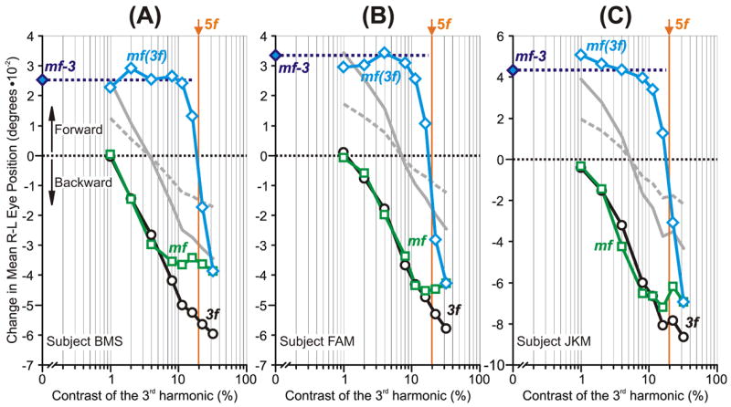
Fig. 2 — The initial OFRs to the mf stimuli: dependence on the contrast of the 3^rd harmonic (mean R-L response measures for each of three subjects). Plots show the OFR elicited by: 1) pure 3f stimuli (black circles), 2) mf stimuli, whose total contrast/amplitude was varied (green squares), 3) mf stimuli, the contrast/amplitude of whose 3^rd harmonic was varied selectively while the contrasts/amplitudes of all other harmonics were held constant at the level they had when the 3^rd harmonic was maximal, i.e., 32% (blue diamonds, labeled *mf(3f)*). The responses to the mf stimulus lacking the 3^rd harmonic (*mf-3* stimulus) are plotted on the vertical axes (filled blue diamonds and extrapolated horizontal dashed lines). Also shown are the simulated *mf(3f)* responses based on the vector sum (grey continuous lines) and vector average (grey dashed lines) of the responses to the *mf-3* and 3f stimuli. The contrast of the 5^th harmonic is shown in vertical orange lines (labeled, 5f). A: subject BMS (147–164 trials per condition; SD’s ranged 0.017–0.025°). B: subject FAM (197–209 trials per condition; SD’s ranged 0.017–0.022°). C: subject JKM (195–219 trials per condition; SD’s ranged 0.023–0.032°). Responses in the forward direction are positive.

This importance of the 3^rd harmonic of the mf stimulus became even more apparent when its contrast was the sole dependent variable. For this we used the mf(3f) stimulus—whose 5^th and higher harmonics always exactly matched those of the mf stimulus when its 3^rd harmonic had a contrast of 32%—and selectively reduced the contrast of its 3^rd harmonic. Selectively halving the contrast of the 3^rd harmonic of the mf(3f) stimulus (from 32% to 16%) had a much more dramatic impact on the initial OFR—actually reversing its direction (see the blue diamonds in Fig. 2)—than did the same change in the contrast of the pure 3f stimulus. In fact, the change in the initial OFR here was, on average, almost nine times greater with the mf(3f) stimulus than with the pure 3f stimulus. The reversal in the OFR occurred as the contrast of the 3^rd harmonic fell below the contrast of the 5^th harmonic, which was now the principal Fourier component with a contrast of ~19%, i.e., ~60% of the contrast of the 3^rd harmonic when the latter was maximal: see the vertical orange lines labeled “5f” in Fig. 2. However, when the contrast of the 3^rd harmonic was reduced further to 8%, so that it was now <½ the contrast of the 5^th harmonic, the initial OFR now began to asymptote, i.e., to settle very close to the OFR recorded when the 3^rd harmonic had zero contrast: see the filled blue diamonds and associated horizontal dashed lines labeled “mf-3” in Fig. 2. Indeed, selectively reducing the contrast of the 3^rd harmonic of the mf(3f) stimulus from 8% to 1% had little or no impact on the initial OFR—especially in subjects BMS and FAM—whereas the same reduction in the contrast of the pure 3f stimulus had a substantial impact.

In summary, the initial OFR elicited by the mf stimulus was determined largely by its 3^rd harmonic, but when the contrast of that harmonic was selectively reduced so that it was less than ~½ that of the next most prominent harmonic, the 5^th, then that 3^rd harmonic effectively lost most of its influence and the OFR was now largely determined by the higher harmonics.

2.3. Discussion of Experiment 1

The abrupt reversal of the initial OFR when the contrast of the 3^rd harmonic of the mf(3f) stimulus was selectively reduced below that of the 5^th harmonic reinforces our earlier suggestion that the OFR depends critically on the Fourier composition of the stimulus (Sheliga et al., 2005), and is consistent with the idea that the initial OFR relies on sensors that respond to a spatially filtered version of the motion stimulus as in the 1^st-order motion energy model (Adelson & Bergen, 1985; van Santen & Sperling, 1985; Watson & Ahumada, 1985). However, a vector sum or vector average of the responses to the mf-3 and 3f stimuli provided very poor fits to the mf(3f) data: see the grey continuous and dashed lines, respectively, in Fig. 2. The relative insensitivity to the 3^rd harmonic of the mf(3f) stimulus when that harmonic’s contrast was less than ½ that of the 5^th harmonic indicates that there is a nonlinear interaction between the neural mechanisms sensing the motion of the two major harmonics that effectively eliminates the influence of the one with the lower contrast: winner-take-all. Our remaining experiments used specially designed visual stimuli to explore some fundamental properties of these nonlinear interactions.

3. Experiment 2: The initial OFR to the 3f5f stimulus and its dependence on the relative contrasts of the two components

Experiment 1 used broadband mf stimuli, yet most of the discussion centered on the contrast of the two principal harmonics—the 3^rd and 5^th. In Experiment 2 we simplified the situation by reducing the stimulus to just two sine waves with spatial frequencies in the ratio 3:5 corresponding to the 3^rd and 5^th harmonics of the mf stimuli. Apparent motion again consisted of successive steps that were each ¼ of the fundamental wavelength, so that the 5f component moved forwards in steps that were each ¼ of its wavelength while the 3f component moved backwards in steps that were each ¼ of its wavelength. The contrast of the 5f component was fixed at one of several levels while the contrast of the 3f component was varied systematically over a wide range. The actual spatial frequencies used were chosen so that, in isolation, the two sine-wave stimuli had roughly equal efficacy when of equal contrast. We report that when the contrast of one component was less than half that of the other then the initial OFR was dominated by the component with the higher contrast and the component with the lesser contrast was almost totally without influence: winner-take-all. On the other hand, when the contrasts of the two components were more similar then both components contributed to the resultant OFR: vector sum/average. In these experiments, the total contrast always covaried with the contrast of the 3f component, but an additional control experiment—in which the total contrast was fixed and the relative contrasts of the two component gratings were varied—yielded very similar data.

3.1. Methods

Most of the methods and procedures were identical to those used in Experiment 1, and only those that were different will be described here.

3.1.1. Visual display

The visual images consisted of one-dimensional vertical grating patterns produced by summing together two sine waves with spatial frequencies in the ratio 3:5, creating a beat of spatial frequency, f: “the 3f5f stimulus”. The spatial frequency of the fundamental was 0.065 cycles/° (wavelength, 15.3°), so that the spatial frequencies of the 3f and 5f components were 0.196 cycles/° and 0.327 cycles/° (wavelengths, 5.1° and 3.06°), respectively. Again, the intention was to select two spatial frequencies that were at symmetrical locations on either side of the peak of the spatial-frequency tuning curve for the OFR so that the two components were of similar efficacy when of equal contrast. The successive phase shifts used to generate the apparent motion always had the same absolute amplitude, 3.825°, which was ¼ of the fundamental wavelength of the 3f5f stimulus, so that the 3f component effectively moved backwards in steps that were each ¼ of its wavelength and the 5f component effectively moved forwards in steps that were each ¼ of its wavelength (spatial aliasing), cf., the 3^rd and 5^th harmonics of the mf stimuli in Experiment 1. The apparent speed of the 3f5f stimuli was 382.5°/s and the total displacement was 76.5°. In any given trial, the Michelson contrast of the 5f component was fixed at one of 5 levels (0%, 4%, 8%, 16%, 32%) while the Michelson contrast of the 3f component was fixed at one of 15–24 levels (ranging from 0–64%), and each was randomly sampled each trial from a lookup table.

3.1.2. Procedures

These were as in Experiment 1 except that each block of trials had 172 randomly interleaved stimulus combinations: 5 contrasts for the 5f component, 15–24 contrasts for the 3f component and 2 directions of motion.

3.2. Results

3.2.1. The main experiment

The complete set of data for all three subjects is shown in Fig. 3, in which the mean R-L response measures are plotted against the contrast of the 3f component of the 3f5f stimulus (logarithmic abscissa). The contrast of the 5f component was fixed at one of five levels ranging from 0% to 32% (indicated by the five different colors in Fig. 3). When the contrast of the 5f component was fixed at zero, the initial OFRs obtained with the (pure) 3f stimuli were as in Experiment 1, i.e., responses were always in the backward direction and the mean R-L response measures showed a roughly linear dependence on log contrast: see the black circles in Fig. 3. The control data obtained with the pure 5f stimuli—when the contrast of the 3f component was zero—are plotted on the vertical axes ¹ of Fig. 3 (see also the colored horizontal dotted lines extending from these data points). As expected, the OFRs to these pure 5f stimuli were all in the forward direction, hence their mean R-L response measures are positive in our sign convention. As pointed out in the Methods, the particular spatial frequencies that were used were specifically chosen so that the pure 3f and 5f stimuli would have comparable efficacy for the OFR (see Methods) and we were reasonably successful in this. Thus, there were four contrasts (4%, 8%, 16%, 32%) for which we collected data for both the 3f and the 5f stimuli, and the ratio of the mean R-L response measures to matching contrasts, R_3f/R_5f, showed no consistent dependence on contrast and a mean value (±1 SD) for the 3 subjects of 1.09±0.12, indicating that the pure 3f stimuli were generally slightly more effective than the pure 5f stimuli.

Apropos the experiments with the 3f5f stimulus, we will first describe the data obtained when the contrast of the 5f component was fixed at 4% (blue filled circles in Fig. 3). The addition of a 3f component to this 5f component was almost without impact until its contrast reached 3% or more (i.e., the OFRs remained close to those obtained with the pure 5f stimulus), even though the OFRs to the pure 3f stimulus showed a clear dependence on contrast over this range. As the contrast of the 3f component of the 3f5f stimulus was increased further to 4%, so that it now matched the contrast of the 5f component, the initial OFR abruptly declined towards zero, indicating that the two components of the 3f5f stimulus were now of similar efficacy and generally cancelled one another. Further increase in the contrast of the 3f component now resulted in reversal of the OFR and, as its contrast exceeded about 8% (i.e., about twice the contrast of the 5f component), the 3f5f data merged with the data for the pure 3f stimulus. Indeed, as the contrast of the 3f component of the 3f5f stimulus increased from 8% to 64% the data were virtually indistinguishable from those obtained with the pure 3f stimulus, indicating that the 5f component of the 3f5f stimulus was almost without influence over this contrast range.

The other curves in Fig. 3 show the data obtained when the 5f component of the 3f5f stimulus was fixed at higher contrast levels and it is evident that they all followed a very similar pattern—an initial plateau followed by an abrupt transition and gradual merger with the pure 3f data—as dominance shifted from one component to the other. (Though the merger was less clear when the 5f component was fixed at the higher contrast levels because of the limited range of contrasts possible for the 3f stimuli/components.)

We indicated above that the initial OFRs elicited by pure 3f stimuli were invariably slightly greater (on average, by 9%) than the initial OFRs elicited by pure 5f stimuli of the same contrast. The grey lines in Fig. 3, which link each of the 4 data points for which the 3f and 5f components of the 3f5f stimuli had equal contrast, indicate that in two cases—the 4% data for BMS and FAM—there was no OFR, i.e., the two components exactly cancelled one another, but in all other cases there was an OFR and it was always in the forward direction, i.e., in the direction of the 5f component. In fact, all of the three grey lines have a positive slope, indicating that the initial OFR increasingly favored the 5f component as contrast increased.

To further examine the abrupt transitions from dominance by the 5f component to dominance by the 3f component, we computed a Response Ratio and plotted it against the Contrast Ratio. The Response Ratio was given by the following expression:

\frac{R_{3 f 5 f} - R_{3 f}}{R_{5 f} - R_{3 f}}

(1)

where R_3f5f is the mean R-L response to the 3f5f stimulus when the 3f and 5f components have particular contrast values, and R_3f and R_5f are the mean R-L responses to pure 3f and 5f stimuli with contrasts matching those values. To the extent that the response to the compound stimulus is determined exclusively by the 5f component (i.e., R_3f5f ≈ R_5f), the value of the numerator in Expression 1 will approach the value of the denominator and the Response Ratio will therefore approach unity. To the extent that the response to the compound stimulus is determined exclusively by the 3f component (i.e., R_3f5f ≈ R_3f), the value of the numerator in Expression 1 will approach zero and the Response Ratio will therefore also approach zero. In Fig. 4A–C, the data from Fig. 3 have been replotted to show the Response Ratio as a function of the Contrast Ratio (on a log scale), where the latter is given by the contrast of the 3f component divided by the contrast of the 5f component. It is now clear that the transition from dominance by the 5f component—when the Response Ratio approached unity—to dominance by the 3f component—when the Response Ratio approached zero—was both abrupt and relatively independent of the absolute contrast of the 5f component.

The amplitudes of the OFRs (on individual trials) to a given 3f5f stimulus were normally distributed, being well fit by a Gaussian function with r² values generally in the range 0.8–1.0: see the mean r² values plotted in black in Fig. 4G–I. The SDs of these Gaussian fits are plotted in black in Fig. 4D–F and show a slightly V-shaped dependence on the Contrast Ratio with a minimum near the center of the transition zone when the Contrast Ratio was close to 1 (and when the OFR amplitudes were close to minimal). We will return to these response distributions later when we discuss the etiology of the responses in the transition zone.

To obtain a quantitative estimate of the abruptness of the transitions in Fig. 4A–C, each of the 4 data sets for each subject was fitted with a Cumulative Gaussian function using a least squares criterion: see the smooth colored lines in these graphs. The r² values for these fits averaged 0.990 (range, 0.980–0.998), indicating that they provide a very adequate description of these data, and their major parameters are plotted as a function of the contrast of the 5f component in Fig. 5 (open symbols). The SDs of the Cumulative Gaussians (Fig. 5A) showed no consistent dependence on the contrast of the 5f component, i.e., the transition was mostly determined by the Contrast Ratio over a wide range of absolute contrasts. The amplitudes of the Cumulative Gaussians (Fig. 5B) were often less than unity (mean, 0.94) and showed a slight tendency to decrease with increases in the contrast of the 5f component. When fitted to the total data set pooled from all three subjects (and forced through 0 and 1), the Cumulative Gaussian had an SD of 0.15 log units (r²=0.98), indicating that, on average, the Response Ratio ranged from 0.05 to 0.95 as the Contrast Ratio ranged from 0.62 to 2.03. Thus, in general, one component of the 3f5f stimulus effectively lost its influence on the initial OFR when its contrast was less than about half that of the other component.

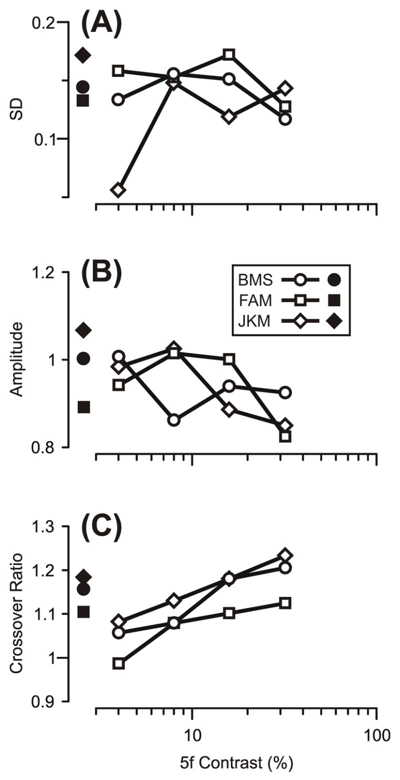
Fig. 5 — Dependence of the Response Ratio on the Contrast Ratio for the *3f5f* data: Parameters of the best-fit Cumulative Gaussian functions and their dependence on the contrast of the 5f component (three subjects). A: Standard Deviation (SD) of the Cumulative Gaussian. B: Amplitude of the Cumulative Gaussian. C: Crossover Ratio of the Cumulative Gaussian, defined as the Contrast Ratio at which the 3f and 5f components cancel, i.e., at which Response Ratio=0.5. Open symbols: data obtained with the standard paradigm. Closed symbols: data obtained with the constant-total-contrast paradigm. Circles, subject BMS. Squares, subject FAM. Diamonds, subject JKM.

The Cumulative Gaussian functions were also used to obtain estimates of the Contrast Ratios when the Response Ratios had a value of 0.5, i.e., when the two components of the 3f5f stimulus exactly cancelled one another. These Contrast Ratios, which we termed “the Crossover Ratios”, are plotted in Fig. 5C and provide a measure of the relative efficacies of the two components of the 3f5f stimuli. The Crossover Ratios were generally slightly greater than unity and increased with increases in the contrast of the 5f component, once more indicating that the 5f component generally had a slightly greater efficacy than the 3f component and especially at the higher contrasts, cf., the grey lines in Fig. 3.

3.2.2. A control experiment in which the total contrast of the 3f5f pattern was kept constant

Experiment 2 employed two sine waves with competing motions and examined the response transition as the contrast of one sine wave was gradually changed while the contrast of the other was held constant. One potentially unfortunate consequence of this experimental design is that the changes in the contrast of the 3f component in Fig. 3 (and the changes in the Contrast Ratio in Fig. 4) were accompanied by changes in the overall contrast of the 3f5f pattern. This raised the possibility that contrast normalization (Carandini & Heeger, 1994; Carandini, Heeger & Movshon, 1997; Heeger, 1992; Heuer & Britten, 2002) contributed to the transitions in these two plots, though this seems unlikely to have been very significant because the SDs of the Cumulative Gaussians showed no clear dependence on the absolute contrast of the 5f component. To address this issue directly we repeated Experiment 2 using 3f5f stimuli whose total contrast was fixed at 32% so that increases in the contrast of one component were balanced by decreases in the contrast of the other component. The 3f and 5f components of the 3f5f stimulus could have one of 15 Contrast Ratios selected randomly from a lookup table: 0.125, 0.25, 0.3536, 0.5, 0.5946, 0.7071, 0.8409, 1.0, 1.1892, 1.4142, 1.6818, 2.0, 2.8284, 4.0, and 8.0.

The data obtained with the constant-contrast 3f5f stimuli were very similar in all essentials to those obtained in Experiment 2. Thus, the plots of the Response Ratio against the Contrast Ratio were well fit by Cumulative Gaussians (r²=0.99 for all 3 subjects) whose parameters were generally within the range of values obtained in Experiment 2: see the filled symbols plotted near the vertical axes in Fig. 5.

3.3. Discussion of Experiment 2 and the associated control experiment

The data in Figs. 3 and 4 indicate that when two superimposed sine waves differing in spatial frequency and speed moved in opposite directions, the resulting OFR depended critically on the relative contrasts of those two sine waves, and this dependence was highly nonlinear, involving an abrupt transition from dominance by one sine wave to dominance by the other. Thus, when the two components of the 3f5f stimulus differed in contrast by more than an octave then the component with the lower contrast lost its influence on the initial OFR: winner-take-all. A control experiment, in which the overall contrast of the 3f5f stimulus was kept constant, indicated that this transition was not due to a non-specific contrast-normalization process.

Like previous authors who described winner-take-all behavior (Ferrera, 2000; Ferrera & Lisberger, 1995; 1997; Recanzone & Wurtz, 1999), we suggest that it reflects nonlinear interactions in the form of mutual inhibition between motion-sensitive channels that are selectively sensitive to opposite directions of motion (and, in our case, possibly also selectively sensitive to different spatial frequencies and/or speeds). In its most extreme form, the mutual inhibition might be so powerful that the response on any given trial is exclusively driven by only one of the two components. This seems likely to have been the situation when the Contrast Ratio was <0.5 or >2 and resulted in Response Ratios close to unity and zero, respectively. However, if a winner-take-all arrangement prevailed in the transition zone—when the Contrast Ratio was between 0.5 and 2.0—then a Response Ratio of 0.7, for example, would mean that the OFR was effectively driven exclusively by the 5f component in ~70% of the trials and exclusively by the 3f component in ~30% of the trials. If this were the case, then we might expect the distributions of the OFRs to the 3f5f stimuli to be much broader—perhaps even bimodal in some extreme cases—inside the transition zone than outside. We examined this issue quantitatively by simulating the response distributions predicted by the winner-take-all model in the transition zone, using the known distributions of the responses to the pure 3f and 5f stimuli, and an example is shown in Fig. 6A, B. The histograms in Fig. 6A show the distributions of the initial OFRs (based on the raw position measures rather than the R-L measures) obtained with the following stimuli: 1) a leftward pure 3f stimulus of contrast 19% (orange plot), 2) a rightward pure 5f stimulus of contrast 16% (green plot), and 3) a 3f5f stimulus whose 3f and 5f components had matching directions and contrasts (black/gray plot). The best-fit Gaussians for those distributions are also shown in continuous thick line. We used the mean OFRs to the 3 stimuli and Expression 1 to estimate the Response Ratio (0.44), and then simulated the response distribution predicted by the winner-take-all model for the 3f5f stimulus by summing the response distributions obtained with the pure 3f and 5f stimuli, weighted in accordance with this Response Ratio: see the blue histogram and best-fit Gaussian function in Fig. 6B labeled, “3f+5f”. It is clear from this that the simulated “3f+5f” response distribution in Fig. 6B is much broader than the real 3f5f response distribution, which is also shown in Fig. 6B (in grey/black) to facilitate the comparison. That the data in Fig. 6B were typical of the distributions in the transition zone is apparent from the parameters of the best-fit Gaussian functions for all of the simulated “3f+5f” data, which are plotted in red in Fig. 4D–F (SDs) and Fig. 4G–I (r² values). These plots indicate that, inside the transition zone, the simulated winner-take-all data had significantly higher SDs and (sometimes) slightly lower r² values than the actual data (inside or outside the transition zone). In fact, there is a slight tendency for the SDs of the best-fit Gaussians for the real 3f5f data in Fig. 4D–F to be minimal in the transition zone (probably in large part because the trial-by-trial response variability depends on the response amplitude). These findings are all consistent with the idea that vector sum/averaging prevails at the center of the transition zone and gradually shifts towards winner-take-all as the Contrast Ratio approaches the boundaries of this zone. Interestingly, the pursuit data of Ferrera (2000) could shift from vector averaging to winner-take-all gradually over time within a given trial.²

Fig. 6 — The initial OFRs to the *3f5f* stimuli: simulation of the response distributions to particular stimuli based on the winner-take-all model. A: Histograms of the distributions of the response measures obtained from subject BMS with leftward pure 3f stimuli of contrast 19% (orange plot), rightward pure 5f stimuli of contrast 16% (green plot), and the *3f5f* stimulus whose 3f and 5f components had matching directions and contrasts (grey plot); smooth curves are best-fit Gaussian functions. B: Histograms of the simulated “3f+5f” distributions for subject BMS obtained by summing the measured distributions for the leftward pure 3f stimuli and the rightward pure 5f stimuli but weighted in accordance with the measured Response Ratio of 0.44 (blue plot). Histograms were binned using custom Matlab subroutines in which the optimal bin width for each individual distribution was given by *2(IQR) N*⁻*^1/3*, where *IQR* is the interquartile range (the 75th percentile minus the 25th percentile) and N is the number of samples.

The relative efficacies of the 3f and 5f components near the center of the transition zone were assessed in two ways: first from the residual responses when the two components of the 3f5f stimulus had the same contrast (data points linked by grey lines in Fig. 3), and second from the Crossover Points in the Cumulative Gaussian functions which indicated the Contrast Ratios when the two components of the 3f5f stimulus exactly cancelled (Fig. 5C). Both indicated that the 5f component had the slightly greater efficacy, especially with higher contrast stimuli, despite the fact that the pure 3f and 5f stimuli had roughly equal efficacy when of equal contrast (by design). For example, when the 5f component of the compound stimulus had a contrast of 32%, the Crossover Point indicated that its efficacy exceeded that of the 3f component, on average, by 19±6% (±SD). On the other hand, with pure sinewave stimuli of contrast 32%, the OFRs to the 3f stimuli were, on average, greater than those to the 5f stimuli by 4±6% (±SD). We suggest that this change in the relative efficacies of the two sine waves when they are combined reflects inequalities in the nonlinear interactions between their motion sensors, that is, differences in the strengths of the inhibition that they exert upon one another. Thus, the suggestion is that the sensors mediating the motion of the 5f component exert more inhibition on the sensors mediating the 3f motion than vice versa, especially at higher contrasts.

A number of recent studies of saccadic eye movements have confronted the subject with more than one target and have used weighted-average models to account for the associated nonlinearities (Krommenhoek & Wiegerinck, 1998; McGowan, Kowler, Sharma & Chubb, 1998; Port & Wurtz, 2003; Walton, Sparks & Gandhi, 2005). We therefore sought to determine how well the curves in Fig. 3 were fitted by the following simple Contrast-Weighted-Average model with only two free parameters:

{\vec{R}}_{3 f 5 f} = \frac{{(C_{3 f})}^{n_{3 f}}}{{(C_{3 f})}^{n_{3 f}} + {(C_{5 f})}^{n_{5 f}}} {\vec{R}}_{3 f} + \frac{{(C_{5 f})}^{n_{5 f}}}{{(C_{3 f})}^{n_{3 f}} + {(C_{5 f})}^{n_{5 f}}} {\vec{R}}_{5 f}

(2)

where R⃗₃_f ₅_f is the simulated OFR to a 3f5f stimulus whose components have contrasts of C₃_f and C₅_f, respectively; R⃗₃_f and R⃗₅_f are the measured OFRs to pure 3f and 5f stimuli, respectively, with contrasts of C₃_f and C₅_f, respectively; n_3f and n_5f are two free parameters that reflect the efficacies of the 3f and 5f components, respectively, of the 3f5f stimuli and thereby determine the abruptness of the transition. The least squares best-fit values of the n_3f and n_5f parameters, together with the r² values indicating the goodness of the fits, for all of the data curves in Fig. 3 are listed in Table 1. The r² values ranged from 0.983 to 0.997 with a mean of 0.993, indicating that Equation 2 provided a very good and complete description of the data. The exponents provide an estimate of the strengths of the mutual inhibition between the two sine-wave gratings. In 11 of 12 cases, n_5f >n_3f, consistent with the Crossover Ratios, which indicated that the 5f component of the 3f5f stimulus usually had a slightly greater efficacy than the 3f component, even though the OFRs to the pure 3f and 5f stimuli usually showed a very slight bias in the reverse direction. If both exponents were given the same value then the fits got progressively worse as the contrast of the 5f component increased. In sum, the Contrast-Weighted-Average model, with only two free parameters, provided a very good description of our data and captured some important details of the nonlinear interactions.

Table 1.

The weighted average model (Equation 2): least squares best fit parameters for the 3f5f data.

Subject	5f contrast	n_3f	n_5f	r²
BMS	4%	5.48	5.69	0.994
	8%	3.44	3.53	0.991
	16%	4.29	4.55	0.997
	32%	5.38	5.70	0.990
FAM	4%	4.51	4.40	0.993
	8%	5.04	5.22	0.995
	16%	4.33	4.49	0.995
	32%	3.78	3.91	0.983
JKM	4%	12.45	13.20	0.995
	8%	5.22	5.56	0.993
	16%	4.58	4.85	0.991
	32%	3.86	4.10	0.995
Mean± SD		5.20±2.38	5.43±2.55	0.993±0.004

Open in a new tab

4. Experiment 3: The initial OFR to the mf-5 stimulus and its dependence on the contrast of the third harmonic

Experiments 1 and 2 used stimuli whose two principal harmonic components moved in opposite directions and evidence was presented that these were processed by neural mechanisms showing winner-take-all behavior when their two contrasts differed by more than about an octave and gradually shifted towards vector sum/averaging as their contrasts became more similar. We next recorded the initial OFR elicited by ¼-wavelength steps applied to a mf stimulus that lacked the 5^th harmonic, so that the principal Fourier components were the 3^rd and 7^th harmonics, which are both 4n−1 harmonics that each step ¼ of their wavelength in the same backward direction but at different speeds: see Fig. 1D–F. We report that selectively reducing the contrast of the 3^rd harmonic—so that the more-slowly-moving 7^th harmonic became the principal Fourier component—had the effect of reducing the amplitude of the initial OFR until the contrast of that 3^rd harmonic reached less than half that of the 7^th harmonic. At this point, the OFR began to asymptote as the 3^rd harmonic lost its influence and OFR was now determined mostly by the more-slowly-moving 7^th and higher harmonics: winner-take-all.

4.1. Methods

The subjects, as well as most of the methods and procedures, were identical to those used in Experiment 1, and only those that were different will be described here.

4.1.1. Visual display

4.1.2. Procedures

These were as in Experiment 1 except that each block of trials had 40 randomly interleaved stimulus combinations: 6 contrasts for the mf-5 and mf-5(3f) stimuli, 8 contrasts for the 3f stimuli, and 2 directions of motion.

4.2. Results

The initial OFR elicited by successive ¼-wavelength shifts applied to the mf-5 stimuli were invariably in the backward direction (i.e., in the direction of the principal Fourier component, the 3^rd harmonic) and approximated the initial OFR elicited by the same shifts when applied to 3f stimuli whose contrasts matched those of the 3^rd harmonic. This is clear from the R-L response measures plotted for each of the three subjects in Fig. 7: the data obtained with the 3f stimuli (black circles) showed a roughly linear dependence on log contrast (cf., Experiments 1 and 2), and the data obtained with the mf-5 stimuli (green squares), which are plotted with respect to the contrast of their 3^rd harmonic, generally shared a very similar dependence (cf., Sheliga et al., 2005). Selectively reducing the contrast of the 3^rd harmonic of the mf-5(3f) stimulus from its maximum of 32% down to 8% reduced the initial OFR somewhat more than did the same reduction in the contrast of the pure 3f stimulus: see the blue diamonds in Fig. 7. In fact, the change in the initial OFR here with the mf-5(3f) stimulus was, on average, 87% greater than with the pure 3f stimulus. A critical factor here was that the 7^th harmonic, whose contrast was 13.7% in our mf-5(3f) stimuli, now became the most prominent Fourier component: see the vertical orange lines labeled “7f” in Fig. 7. With further selective reductions in the contrast of the 3^rd harmonic, the initial OFR began to asymptote close to the level recorded when the 3^rd harmonic had zero contrast (indicated by the filled blue diamonds and associated horizontal dashed lines labeled “mf-3&5” in Fig. 7), though the 3 subjects showed noticeable differences in this range and, in the case of FAM, substantial variability. The change in OFR as the contrast of the 3^rd harmonic was selectively reduced from 4% to 1% was, on average, less than 30% of that when the pure 3f stimulus underwent the same change in contrast.

Fig. 7 — The initial OFRs to the *mf-5* stimuli: dependence on the contrast of the 3^rd harmonic (mean R-L response measures for each of three subjects). Plots show the OFR elicited by: 1) pure 3f stimuli (black circles), 2) *mf-5* stimuli, whose total amplitude/contrast was varied (green squares), and 3) *mf-5* stimuli, the amplitude/contrast of whose 3^rd harmonic was varied selectively while the amplitudes of all other harmonics were held constant at the level they had when the 3^rd harmonic was maximal, i.e., 32% (blue diamonds, labeled *mf-5(3f)*). The responses to the *mf-5* stimulus lacking the 3^rd harmonic (*mf-3&5* stimulus) are plotted on the vertical axes (filled blue diamonds and extrapolated horizontal dashed lines). The contrast of the 7^th harmonic is shown in vertical orange lines (labeled, 7f). A: subject BMS (144–164 trials per condition; SD’s ranged 0.018–0.025°). B: subject FAM (198–210 trials per condition; SD’s ranged 0.016–0.021°). C: subject JKM (191–219 trials per condition; SD’s ranged 0.023–0.032°). Other conventions as in Fig. 2.

4.3. Discussion of Experiment 3

The data obtained in Experiment 3 resembled those obtained in Experiment 1: selectively reducing the contrast of the major harmonic of a broadband stimulus resulted in an abrupt transition in the initial OFR as that harmonic ceded control to the next largest harmonic. However, the transition was not as abrupt and the subsequent asymptote was not as clear-cut as in the earlier experiment. Nonetheless, the reduced sensitivity to the 3^rd harmonic when its contrast fell substantially below that of the 7^th harmonic suggests that again there is a winner-take-all arrangement, though perhaps involving somewhat weaker mutual inhibition between the neural mechanisms sensing the motions of the two harmonics. Of course, a major difference in the present experiment was that the two harmonics in question were moving in the same rather than the opposite direction. Thus, discrimination between the two motions here requires neural mechanisms that differ in their spatial frequency tuning and/or speed tuning.

5. Experiment 4: The initial OFR to the 3f7f stimulus and its dependence on the relative contrasts of the two components

Experiment 3 used the broadband mf-5 stimulus but, as with the mf stimulus in Experiment 1, most of the discussion was restricted to the two most prominent harmonics, so we again attempted to gain further insights by using stimuli consisting of only two sine waves, this time with spatial frequencies in the ratio 3:7 corresponding to the 3^rd and 7^th harmonics of the mf-5 stimulus. Using the usual ¼-wavelength steps, so that the 3f and 7f components each moved backwards in steps that were ¼ of their respective wavelengths, we again report that when the contrast of one component exceeded that of the other by a certain amount then the component with the lesser contrast lost its influence on the initial OFR: winner-take-all. These effects were only slightly less robust than those reported in Experiment 2 when the two sine waves moved in opposite directions.

5.1. Methods

Most of the methods and procedures were identical to those used in Experiment 1, and only those that were different will be described here.

5.1.1. Subjects

Three subjects participated: one was an author (FAM) and the others were paid volunteers who were unaware of the purpose of the experiments (JKM, NPB). All had normal or corrected-to-normal vision. Viewing was binocular for FAM and NPB, and monocular for JKM (right eye viewing).

5.1.2. Visual display

The visual images consisted of one-dimensional vertical grating patterns produced by summing together two sine waves with spatial frequencies in the ratio 3:7, creating a beat of spatial frequency, f: “the 3f7f stimulus”. The spatial frequency of the fundamental was 0.055 cycles/° (wavelength, 18.2°), so that the spatial frequencies of the 3f and 7f components were 0.165 cycles/° and 0.385 cycles/° (wavelengths, 6.067° and 2.6°), respectively. Again, the intention was to select two spatial frequencies that were at symmetrical locations on either side of the peak of the spatial-frequency tuning curve so that the two components were of similar efficacy. However, spatial-frequency tuning curves were only available for two of the three subjects (FAM, JKM). The successive phase shifts used to generate the apparent motion always had the same absolute amplitude, 4.55°, which was ¼ of the fundamental wavelength of the 3f7f stimulus, so that the 3f and 7f components effectively moved backwards in steps that were each ¼ of their wavelengths (spatial aliasing), cf., the 3^rd and 7^th harmonics of the mf-5 stimuli in Experiment 3. The apparent speed of the 3f7f stimuli was 455°/s and the total displacement was 91°. In any given trial, the Michelson contrast of the 7f component was fixed at one of 5 levels (0%, 4%, 8%, 16%, 32%) while the Michelson contrast of the 3f component was fixed at one of 15–24 levels (ranging from 0–64%), randomly sampled each trial from a lookup table.

5.1.3. Procedures

These were as in Experiment 1 except that each block of trials had 172 randomly interleaved stimulus combinations: 5 contrasts for the 7f component, 15–24 contrasts for the 3f component and 2 directions of motion.

5.2. Results

The complete set of data for all three subjects is shown in Fig. 8, in which the mean R-L response measures are plotted against the contrast of the 3f component of the 3f7f stimulus (logarithmic abscissa). The contrast of the 7f component was fixed at one of five levels ranging from 0% to 32% (indicated by the five different colors in Fig. 8). The data obtained with the pure 7f stimuli, i.e., when the contrast of the 3f component was zero, are plotted as colored symbols on the vertical axes (see also the colored horizontal dotted lines extending from these data points). As expected, the OFRs to these pure 7f stimuli were all in the backward direction, hence their mean R-L response measures were negative in our sign convention. When the contrast of the 7f component was fixed at zero, the initial OFRs obtained with the (pure) 3f stimuli were as in the previous experiments, i.e., responses were always in the backward direction and showed a roughly linear dependence on log contrast: see the black circles in Fig. 8. Regarding the relative efficacies of the pure 3f and 7f stimuli, the ratio of the mean R-L response measures to matching contrasts, R_3f/R_7f, showed no consistent dependence on contrast and a mean value (±1 SD) for subjects FAM and JKM of 1.10±0.08, indicating that the pure 3f stimuli were generally slightly more effective than the pure 7f stimuli in these subjects. However, for the 3^rd subject (NPB), this ratio was 1.38±0.07, indicating a rather strong bias in favor of the 3f stimuli.

When the contrast of the 7f component was fixed at some finite value, the dependence of the initial OFR on the contrast of the 3f component was sometimes rather complex and for ease of exposition we will first describe the data obtained from subject NPB: Fig. 8A. For this subject, the addition of the 3f component had little impact until its contrast reached more than half that of the 7f component, i.e., the OFRs remained close to those obtained with the pure 7f stimulus, even though the OFRs to the pure 3f stimulus showed a very clear dependence on contrast over this range: winner-take-all. The effects of further increases in the contrast of the 3f component varied with the contrast of the 7f component: when the latter was 4% (blue filled circles in Fig. 8), the 3f7f data simply merged with the pure 3f-sinewave data, indicating that the 7f component was now without influence, but when the contrast of the 7f component was fixed at 8% (magenta open squares) the 3f7f data tended to gradually “overshoot” the pure 3f-sinewave data a little before merging with them only as the 3f component reached its highest contrast levels; this “overshoot” (and gradual merger) became even more prominent when the contrast of the 7f component was fixed at 16% (orange filled squares) and 32% (green open diamonds), the 3f component here exerting little influence until its contrast actually exceeded that of the 7f component. Thus, when the 7f and 3f components both had contrasts of 32%, the initial OFR was dominated by the 7f component, which is the reverse of the bias when these stimuli were applied in isolation, indicating an imbalance in the strength of the mutual interactions between the detectors sensing these two sine waves.

The 3f7f data from the other two subjects (FAM and JKM) often displayed many of these same general features—an initial plateau when the 3f component had little influence and a later merger with the pure 3f data as the 7f component lost its influence—but there were some notable departures in the details. For example, the initial portions of the curves in Fig. 8B, C (when the contrast of the 3f component is less than that of the 7f) are not always flat and sometimes have values that consistently exceed those to the corresponding pure 7f stimuli: see especially the 4% and 32% data sets in Fig. 8B, C. Further, the later portions of the curves when the 7f component had a contrast of 8% or 16% showed substantially less “overshoot” and merged more closely with the pure 3f-sinewave data. Finally, the data of the subject FAM that were obtained when the 7f component had a contrast of 32% showed no clear tendency to merge with the pure 3f-sinewave data at the higher contrast levels.

To examine the transition from dominance by the 7f component to dominance by the 3f component more closely, we again computed a Response Ratio and plotted it against the Contrast Ratio, as in Experiment 2. The Response Ratio was given by the following expression:

\frac{R_{3 f 7 f} - R_{3 f}}{R_{7 f} - R_{3 f}}

(3)

where R_3f7f is the OFR to the 3f7f stimulus when the 3f and 7f components have particular contrast values, and R_3f and R_7f are the OFRs to pure 3f and 7f stimuli with matching contrast values. When the response to the compound stimulus is determined almost exclusively by the 7f component (i.e., R_3f7f ≈ R_7f), the Response Ratio approaches unity, and when the response to the compound stimulus is determined almost exclusively by the 3f component (i.e., R_3f7f ≈ R_3f), the Response Ratio approaches zero. However, the use of the Response Ratio to characterize the 3f7f data was problematic insofar as R_3f and R_7f could have very similar values so that the denominator of Expression 3 could be small and, hence, very sensitive to noise. For this reason, we discarded those Response Ratios whose denominators had a value <0.03°. This resulted in 59% of the data being discarded, necessitating that we pool the residual data from all three subjects to achieve an adequate sampling over the full range of Contrast Ratios and these pooled data are shown in Fig. 9A. Although based on a relatively small, pooled data sample, the dependence of the Response Ratio on the Contrast Ratio in Fig. 9A clearly resembles those plotted for the 3f5f data in Fig. 4. Thus, the transition from dominance by the 7f component—when the Response Ratio approached unity—to dominance by the 3f component—when the Response Ratio approached zero—was fairly abrupt and relatively independent of the absolute contrast of the 7f component. Again, the data were reasonably well fit by a Cumulative Gaussian (r²=0.89), with a SD of 0.19 log units and a Crossover Ratio of 1.47, indicating once more that the 7f component of the 3f7f stimulus had a substantially greater efficacy than the 3f component, which was the opposite of the bias with the pure 3f and 7f stimuli.

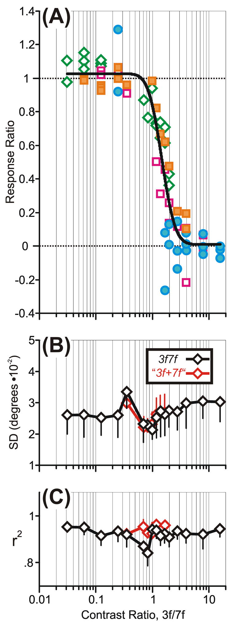
Fig. 9 — The initial OFRs to the *3f7f* stimuli: dependence of the Response Ratio on the Contrast Ratio, *3f/7f* (selected pooled data for three subjects from Fig. 8). A: Response Ratios when the amplitude/contrast of the 3f component was varied systematically while the amplitude/contrast of the 7f component was fixed at 4% (blue filled circles), 8% (magenta open squares), 16% (orange filled squares), and 32% (green open diamonds); continuous smooth curve is best-fit Cumulative Gaussian function. B: Dependence of the mean Standard Deviations of the “best-fit Gaussians for the response distributions to individual *3f7f* stimuli” on the Contrast Ratio (actual data in black, simulated winner-take-all data in red). C: Dependence of “the mean r² values of the best-fit Gaussians for the response distributions to individual *3f7f* stimuli” on the Contrast Ratio (actual data in black, simulated winner-take-all data in red). Error bars, SD.

The amplitudes of the individual OFRs to any given 3f7f stimulus were normally distributed and well fit by a Gaussian function with r² values generally in the range 0.8–1.0: see the mean r² values plotted in black in Fig. 9C. The SDs of these Gaussian fits are plotted in black in Fig. 9B and show somewhat more scatter than the 3f5f data in Fig. 4D–F.

5.3. Discussion of Experiment 4

The data in Fig. 9 indicate that when two superimposed sine waves differing in spatial frequency and speed moved in the same direction the resulting OFR depended critically on the relative contrasts of those two sine waves, and this dependence was highly nonlinear, involving an abrupt transition from dominance by one sine wave to dominance by the other: winner-take-all. Unfortunately, the data in Fig. 9 are pooled from all 3 subjects and represent only a relatively small proportion of the original data set (41%). The SD of the best-fit Cumulative Gaussian for the 3f7f data in Fig. 9A was 0.19 log units, which is only slightly greater than that for the 3f5f data pooled from all three subjects in Experiment 2 (SD=0.15 log units; r²=0.98). This suggests that the transition was only slightly less abrupt with the 3f7f stimuli than with the 3f5f stimuli. Clearly, with the 3f5f stimulus, the neural mechanisms that process the two motion signals separately could be selectively tuned for direction and/or spatial frequency and/or speed, whereas with the 3f7f stimulus, the only useful distinguishing features are spatial frequency and/or speed (though these are more different for the 3f7f stimulus than for the 3f5f stimulus).

In an attempt to determine if the responses in the transition zone resulted from winner-take-all and/or vector sum/averaging, we again simulated the distributions of the OFRs for particular stimuli for the winner-take-all model using the distributions of the responses obtained with the pure 3f and 7f stimuli. The latter were weighted in accordance with the Response Ratio, and then fitted with Gaussian functions whose SDs and r² values are plotted in red in Figs. 9B and 9C, respectively. It is now apparent that the winner-take-all model does not predict a clear difference between the SDs and r² values inside and outside the transition zone with the 3f7f stimuli, hence this approach cannot be used to address the issue of winner-take-all and vector sum/averaging in the transition zone. Presumably, a major factor here is that the response distributions with the pure 3f and 7f stimuli show considerable overlap.

The Crossover Ratio suggested that the 7f component of the 3f7f stimulus had a substantially greater efficacy than the 3f component, whereas the data obtained with the pure 3f and 7f stimuli showed the reverse tendency—especially for subject NPB. As pointed out previously in discussing the 3f5f data, the apparent change in the relative efficacies of the two sine waves when they are combined together can be attributed to inequalities in the nonlinear interactions between the neural mechanisms processing them, and the present findings are consistent with the idea that the mechanisms channeling the motion of the 7f component exert more inhibition on the mechanisms channeling the 3f motion than vice versa. This result is also consistent with the data from Experiment 2 insofar as it is the higher spatial frequency channel that exerts the greater inhibition.

6. General Discussion

A number of studies on monkeys have recorded the initial pursuit eye movements elicited by two discrete moving targets and have reported behavior ranging from vector sum/averaging to winner-take-all depending on the experimental conditions (Ferrera, 2000; Ferrera & Lisberger, 1995; 1997; Lisberger & Ferrera, 1997; Recanzone & Wurtz, 1999). The extent of the winner-take-all here depended on whether there was prior knowledge about which of the targets should be tracked, as well as other features of the stimulus conditions. In these studies, vector averaging was regarded as the default condition, and any bias in favor of one or other target, suggesting a tendency towards winner-take-all, was attributed to selective attention. Ferrera and Lisberger (1995) and Ferrera (2000) simulated these effects with recurrent network models in which competing inputs mutually inhibited one another, and showed that a selection bias—representing the balance of attention between the two targets—could modulate the output continuously from vector averaging to winner-take-all. In all of these pursuit studies, the competing motions involved discrete targets that were of comparable efficacy/contrast and the winner-take-all outcome depended critically on top-down influences. It would be interesting to know if merely altering the relative contrasts of the two pursuit targets could shift the default from vector averaging towards winner-take-all. In fact, the models of Ferrera & Lisberger (1995) and Ferrera (2000) do not distinguish between top-down and bottom-up sources of bias and so would be expected to show winner-take-all if the two targets merely differed sufficiently in contrast.

Whether the outcome is vector averaging or winner-take-all (or intermediate) presumably reflects the mechanisms by which the brain reads out the activity of the populations of neurons that are activated by the visual motion stimuli. In the above-mentioned studies on pursuit eye movements, vector averaging was assumed to result when all of the active neurons in the population make a contribution (summation) and there is a divisive normalization (Carandini & Heeger, 1994; Heeger, Simoncelli & Movshon, 1996; Simoncelli & Heeger, 1998), whereas winner-take-all was assumed to result when only the most active neurons in the population make a contribution. The study of Recanzone and Wurtz (1999) showed that the activity of neurons in MT and MST, which have been strongly implicated in the generation of pursuit eye movements (Dursteler, Wurtz & Newsome, 1987; Groh, Born & Newsome, 1997; Komatsu & Wurtz, 1988; Komatsu & Wurtz, 1989; Newsome, Wurtz, Dursteler & Mikami, 1985; Schiller & Lee, 1994; Yamasaki & Wurtz, 1991) as well as the OFR (Kawano, Inoue, Takemura, Kodaka & Miles, 2000; Kawano, Shidara, Watanabe & Yamane, 1994; Takemura, Inoue & Kawano, 2002) reflected the vector averaging/winner-take-all bias in the pursuit tracking responses. Several studies have also used electrical microstimulation to perturb the neuronal activity in MT while monkeys discriminated the direction of perceived motion of a visual pattern and reported either vector averaging (Groh et al., 1997) or winner-take-all (Salzman & Newsome, 1994) or both (Nichols & Newsome, 2002), depending on the experimental conditions. In this last study of Nichols and Newsome, the directions of the perceived motion associated with the real and the electrical stimuli were varied widely and winner-take-all was evident only when these were in opposite directions.³ Thus, when the two directions of perceived motion differed by 45°, for example, the outcome was invariably vector averaging. Interestingly, Masson and Castet (2002) recently recorded the initial human OFRs elicited by the motion of type I plaid patterns whose component gratings differed in orientation by 45° and found vector averaging. These workers also did an experiment in which they applied the motion to only one of the two components (type II unikinetic plaids) and reported the dependence of the initial OFR on the contrast ratio: their data (see their Fig. 23) show no evidence of any abrupt transition with changes in the contrast ratio and so are again consistent with vector averaging. This clearly suggests that the winner-take-all behavior that we have reported in this paper is restricted to motions that are close to the same plane.

The data in Experiments 1 and 2 suggest the existence of strong mutual inhibition between channels subserving opposite directions of motion. This is often termed, “motion opponency”, and has considerable supporting evidence from psychophysical studies (Levinson & Sekuler, 1975; Mather & Moulden, 1983; Qian, Andersen & Adelson, 1994; Stromeyer, Kronauer, Madsen & Klein, 1984; van Santen & Sperling, 1984; Zemany, Stromeyer, Chaparro & Kronauer, 1998), functional magnetic resonance imaging (Heeger, Boynton, Demb, Seidemann & Newsome, 1999), and single unit recordings in area MT (Bradley, Qian & Andersen, 1995; Mikami, Newsome & Wurtz, 1986; Qian & Andersen, 1994; Rodman & Albright, 1987; Rust, 2004; Snowden, Treue, Erickson & Andersen, 1991). The study of Rust (2004) is of particular interest, describing nonlinear interactions between the responses to contrast-weighted combinations of sinusoids moving in the null and preferred directions of direction-selective neurons in V1 and MT (see also Rust, Schwartz, Movshon & Simoncelli, 2005). The nonlinear interaction took the form of a powerful null-suppression, so that changes in the contrast ratio resulted in abrupt changes in neuronal activity as the balance shifted between the null and preferred stimuli, cf., the abrupt transitions in our study. The suppression was tuned for the null direction, and Rust (2004) concluded that it was exclusive to V1, i.e., MT inherited motion opponency from V1.

While motion opponency might explain our findings in Experiments 1 and 2 it clearly cannot explain those in Experiments 3 and 4. In these cases, the neural mechanisms sensing the two motions must rely on the differences in the spatial frequency and/or speed of the two gratings in order to distinguish between them. There is substantial evidence for mutual inhibition between neurons in striate cortex tuned for different spatial frequencies (e.g., Albrecht & De Valois, 1981; De Valois & Tootell, 1983; Movshon, Thompson & Tolhurst, 1978), though these studies were not specifically concerned with neurons that were direction selective. Interestingly, there is a strong anisotropy in this mutual inhibition whereby the suppression is most often greatest from spatial frequencies that are higher than that which is optimal for exciting the cell (Albrecht & De Valois, 1981; De Valois & Tootell, 1983). In addition, there is psychophysical evidence for selective suppression of low spatial frequencies by higher ones (e.g., McCourt & Foley, 1985; Morrone, Burr & Ross, 1983; Tolhurst, 1972; Tolhurst & Barfield, 1978). These observations might be linked to our finding that, in the center of the transition zone, the mechanisms sensing the 5f and 7f components of our compound gratings generally exerted more inhibition on the mechanisms sensing the 3f motion than vice versa.

We know of no evidence for mutual inhibition between channels defined exclusively on the basis of their speed selectivity. Indeed, “the coding of speed information is poorly understood” (Stone & Thompson, 1992). Tuning for speed is commonplace among neurons in MT, though for many the preferred speed varies with spatial frequency when tested with single sine-wave gratings (Priebe, Cassanello & Lisberger, 2003; Priebe & Lisberger, 2004). Interestingly, when tested with two superimposed sine waves or broad-band stimuli such as square waves, some MT neurons show speed tuning that is closer to form-invariant, an effect attributed to nonlinear interactions (Priebe et al., 2003). Thus, as in the present study, broad-band and dual-grating stimuli uncovered important nonlinearities that were not evident with single sine-wave stimuli.

Acknowledgments

This research was supported by the Intramural Research Program of the NIH, the National Eye Institute.

Footnotes

Note the discontinuities in the otherwise logarithmic abscissas in Fig. 3.

The very earliest responses in the study of Ferrera (2000) showed a tendency toward vector summation, which over a period of 50 ms or so gradually gave way to vector averaging or winner-take-all (or some intermediate form of processing), consistent with the idea that divisive normalization takes time to develop.

Though their technique could not be used to distinguish between vector averaging and winner-take-all when the two motion percepts had exactly the same direction.

References

Adelson EH. Some new motion illusions, and some old ones, analysed in terms of their Fourier components. Investigative Ophthalmology and Visual Science. 1982;34(Suppl):144. Abstract. [Google Scholar]
Adelson EH, Bergen JR. Spatiotemporal energy models for the perception of motion. Journal of the Optical Society of America A. 1985;2:284–299. doi: 10.1364/josaa.2.000284. [DOI] [PubMed] [Google Scholar]
Albrecht DG, De Valois RL. Striate cortex responses to periodic patterns with and without the fundamental harmonics. Journal of Physiology. 1981;319:497–514. doi: 10.1113/jphysiol.1981.sp013922. [DOI] [PMC free article] [PubMed] [Google Scholar]
Baro JA, Levinson E. Apparent motion can be perceived between patterns with dissimilar spatial frequencies. Vision Research. 1988;28:1311–1313. doi: 10.1016/0042-6989(88)90062-4. [DOI] [PubMed] [Google Scholar]
Bradley DC, Qian N, Andersen RA. Integration of motion and stereopsis in middle temporal cortical area of macaques. Nature. 1995;373:609–611. doi: 10.1038/373609a0. [DOI] [PubMed] [Google Scholar]
Brainard DH. The Psychophysics Toolbox. Spatial Vision. 1997;10:433–436. [PubMed] [Google Scholar]
Brown RO, He S. Visual motion of missing-fundamental patterns: motion energy versus feature correspondence. Vision Research. 2000;40:2135–2147. doi: 10.1016/s0042-6989(00)00080-8. [DOI] [PubMed] [Google Scholar]
Carandini M, Heeger DJ. Summation and division by neurons in primate visual cortex. Science. 1994;264:1333–1336. doi: 10.1126/science.8191289. [DOI] [PubMed] [Google Scholar]
Carandini M, Heeger DJ, Movshon JA. Linearity and normalization in simple cells of the macaque primary visual cortex. The Journal of Neuroscience. 1997;17:8621–8644. doi: 10.1523/JNEUROSCI.17-21-08621.1997. [DOI] [PMC free article] [PubMed] [Google Scholar]
Collewijn H, Van Der Mark F, Jansen TC. Precise recording of human eye movements. Vision Research. 1975;15:447–450. doi: 10.1016/0042-6989(75)90098-x. [DOI] [PubMed] [Google Scholar]
De Valois KK, Tootell RB. Spatial-frequency-specific inhibition in cat striate cortex cells. Journal of Physiology. 1983;336:359–376. doi: 10.1113/jphysiol.1983.sp014586. [DOI] [PMC free article] [PubMed] [Google Scholar]
Dursteler MR, Wurtz RH, Newsome WT. Directional pursuit deficits following lesions of the foveal representation within the superior temporal sulcus of the macaque monkey. Journal of Neurophysiology. 1987;57:1262–1287. doi: 10.1152/jn.1987.57.5.1262. [DOI] [PubMed] [Google Scholar]
Ferrera VP. Task-dependent modulation of the sensorimotor transformation for smooth pursuit eye movements. Journal of Neurophysiology. 2000;84:2725–2738. doi: 10.1152/jn.2000.84.6.2725. [DOI] [PubMed] [Google Scholar]
Ferrera VP, Lisberger SG. Attention and target selection for smooth pursuit eye movements. The Journal of Neuroscience. 1995;15:7472–7484. doi: 10.1523/JNEUROSCI.15-11-07472.1995. [DOI] [PMC free article] [PubMed] [Google Scholar]
Ferrera VP, Lisberger SG. The effect of a moving distractor on the initiation of smooth-pursuit eye movements. Visual Neuroscience. 1997;14:323–338. doi: 10.1017/s0952523800011457. [DOI] [PubMed] [Google Scholar]
Gellman RS, Carl JR, Miles FA. Short latency ocular-following responses in man. Visual Neuroscience. 1990;5:107–122. doi: 10.1017/s0952523800000158. [DOI] [PubMed] [Google Scholar]
Georgeson MA, Harris MG. The temporal range of motion sensing and motion perception. Vision Research. 1990;30:615–619. doi: 10.1016/0042-6989(90)90072-s. [DOI] [PubMed] [Google Scholar]
Georgeson MA, Shackleton TM. Monocular motion sensing, binocular motion perception. Vision Research. 1989;29:1511–1523. doi: 10.1016/0042-6989(89)90135-1. [DOI] [PubMed] [Google Scholar]
Groh JM, Born RT, Newsome WT. How is a sensory map read Out? Effects of microstimulation in visual area MT on saccades and smooth pursuit eye movements. The Journal of Neuroscience. 1997;17:4312–4330. doi: 10.1523/JNEUROSCI.17-11-04312.1997. [DOI] [PMC free article] [PubMed] [Google Scholar]
Hays AV, Richmond BJ, Optican LM. A UNIX-based multiple process system for real-time data acquisition and control. WESCON Conference Proceedings. 1982;2:1–10. [Google Scholar]
Heeger DJ. Normalization of cell responses in cat striate cortex. Visual Neuroscience. 1992;9:181–197. doi: 10.1017/s0952523800009640. [DOI] [PubMed] [Google Scholar]
Heeger DJ, Boynton GM, Demb JB, Seidemann E, Newsome WT. Motion opponency in visual cortex. The Journal of Neuroscience. 1999;19:7162–7174. doi: 10.1523/JNEUROSCI.19-16-07162.1999. [DOI] [PMC free article] [PubMed] [Google Scholar]
Heeger DJ, Simoncelli EP, Movshon JA. Computational models of cortical visual processing. Proceedings of the National Academy of Sciences. 1996;93:623–627. doi: 10.1073/pnas.93.2.623. [DOI] [PMC free article] [PubMed] [Google Scholar]
Heuer HW, Britten KH. Contrast dependence of response normalization in area MT of the rhesus macaque. Journal of Neurophysiology. 2002;88:3398–3408. doi: 10.1152/jn.00255.2002. [DOI] [PubMed] [Google Scholar]
Kawano K, Inoue Y, Takemura A, Kodaka Y, Miles FA. The role of MST neurons during ocular tracking in 3D space. International Review of Neurobiology. 2000;44:49–63. doi: 10.1016/s0074-7742(08)60737-0. [DOI] [PubMed] [Google Scholar]
Kawano K, Shidara M, Watanabe Y, Yamane S. Neural activity in cortical area MST of alert monkey during ocular following responses. Journal of Neurophysiology. 1994;71:2305–2324. doi: 10.1152/jn.1994.71.6.2305. [DOI] [PubMed] [Google Scholar]
Komatsu H, Wurtz RH. Relation of cortical areas MT and MST to pursuit eye movements. I. Localization and visual properties of neurons. Journal of Neurophysiology. 1988;60:580–603. doi: 10.1152/jn.1988.60.2.580. [DOI] [PubMed] [Google Scholar]
Komatsu H, Wurtz RH. Modulation of pursuit eye movements by stimulation of cortical areas MT and MST. Journal of Neurophysiology. 1989;62:31–47. doi: 10.1152/jn.1989.62.1.31. [DOI] [PubMed] [Google Scholar]
Krommenhoek KP, Wiegerinck WAJJ. A neural network study of precollicular saccadic averaging. Biological Cybernetics. 1998;78:465–477. doi: 10.1007/s004220050450. [DOI] [PubMed] [Google Scholar]
Levinson E, Sekuler R. Inhibition and disinhibition of direction-specific mechanisms in human vision. Nature. 1975;254:692–694. doi: 10.1038/254692a0. [DOI] [PubMed] [Google Scholar]
Lisberger SG, Ferrera VP. Vector averaging for smooth pursuit eye movements initiated by two moving targets in monkeys. The Journal of Neuroscience. 1997;17:7490–7502. doi: 10.1523/JNEUROSCI.17-19-07490.1997. [DOI] [PMC free article] [PubMed] [Google Scholar]
Masson GS, Busettini C, Yang DS, Miles FA. Short-latency ocular following in humans: sensitivity to binocular disparity. Vision Research. 2001;41:3371–3387. doi: 10.1016/s0042-6989(01)00029-3. [DOI] [PubMed] [Google Scholar]
Masson GS, Castet E. Parallel motion processing for the initiation of short-latency ocular following in humans. The Journal of Neuroscience. 2002;22:5149–5163. doi: 10.1523/JNEUROSCI.22-12-05149.2002. [DOI] [PMC free article] [PubMed] [Google Scholar]
Masson GS, Yang DS, Miles FA. Reversed short-latency ocular following. Vision Research. 2002a;42:2081–2087. doi: 10.1016/s0042-6989(02)00082-2. [DOI] [PMC free article] [PubMed] [Google Scholar]
Masson GS, Yang DS, Miles FA. Version and vergence eye movements in humans: open-loop dynamics determined by monocular rather than binocular image speed. Vision Research. 2002b;42:2853–2867. doi: 10.1016/s0042-6989(02)00334-6. [DOI] [PMC free article] [PubMed] [Google Scholar]
Mather G, Moulden B. Thresholds for movement direction: two directions are less detectable than one. Quarterly Journal of Experimental Psychology A. 1983;35:513–518. doi: 10.1080/14640748308402485. [DOI] [PubMed] [Google Scholar]
McCourt ME, Foley JM. Spatial frequency interference on grating-induction. Vision Research. 1985;25:1507–1518. doi: 10.1016/0042-6989(85)90229-9. [DOI] [PubMed] [Google Scholar]
McGowan JW, Kowler E, Sharma A, Chubb C. Saccadic localization of random dot targets. Vision Research. 1998;38:895–909. doi: 10.1016/s0042-6989(97)00232-0. [DOI] [PubMed] [Google Scholar]
Mikami A, Newsome WT, Wurtz RH. Motion selectivity in macaque visual cortex. I. Mechanisms of direction and speed selectivity in extrastriate area MT. Journal of Neurophysiology. 1986;55:1308–1327. doi: 10.1152/jn.1986.55.6.1308. [DOI] [PubMed] [Google Scholar]
Miles FA, Kawano K, Optican LM. Short-latency ocular following responses of monkey. I. Dependence on temporospatial properties of visual input. Journal of Neurophysiology. 1986;56:1321–1354. doi: 10.1152/jn.1986.56.5.1321. [DOI] [PubMed] [Google Scholar]
Morrone MC, Burr DC, Ross J. Added noise restores recognizability of coarse quantized images. Nature. 1983;305:226–228. doi: 10.1038/305226a0. [DOI] [PubMed] [Google Scholar]
Movshon JA, Thompson ID, Tolhurst DJ. Spatial and temporal contrast sensitivity of neurones in areas 17 and 18 of the cat’s visual cortex. Journal of Physiology. 1978;283:101–120. doi: 10.1113/jphysiol.1978.sp012490. [DOI] [PMC free article] [PubMed] [Google Scholar]
Newsome WT, Wurtz RH, Dursteler MR, Mikami A. Deficits in visual motion processing following ibotenic acid lesions of the middle temporal visual area of the macaque monkey. The Journal of Neuroscience. 1985;5:825–840. doi: 10.1523/JNEUROSCI.05-03-00825.1985. [DOI] [PMC free article] [PubMed] [Google Scholar]
Nichols MJ, Newsome WT. Middle temporal visual area microstimulation influences veridical judgments of motion direction. The Journal of Neuroscience. 2002;22:9530–9540. doi: 10.1523/JNEUROSCI.22-21-09530.2002. [DOI] [PMC free article] [PubMed] [Google Scholar]
Pelli DG. The VideoToolbox software for visual psychophysics: transforming numbers into movies. Spatial Vision. 1997;10:437–442. [PubMed] [Google Scholar]
Pelli DG, Zhang L. Accurate control of contrast on microcomputer displays. Vision Research. 1991;31:1337–1350. doi: 10.1016/0042-6989(91)90055-a. [DOI] [PubMed] [Google Scholar]
Port NL, Wurtz RH. Sequential activity of simultaneously recorded neurons in the superior colliculus during curved saccades. Journal of Neurophysiology. 2003;90:1887–1903. doi: 10.1152/jn.01151.2002. [DOI] [PubMed] [Google Scholar]
Priebe NJ, Cassanello CR, Lisberger SG. The neural representation of speed in macaque area MT/V5. The Journal of Neuroscience. 2003;23:5650–5661. doi: 10.1523/JNEUROSCI.23-13-05650.2003. [DOI] [PMC free article] [PubMed] [Google Scholar]
Priebe NJ, Lisberger SG. Estimating target speed from the population response in visual area MT. The Journal of Neuroscience. 2004;24:1907–1916. doi: 10.1523/JNEUROSCI.4233-03.2004. [DOI] [PMC free article] [PubMed] [Google Scholar]
Qian N, Andersen RA. Transparent motion perception as detection of unbalanced motion signals. II. Physiology. The Journal of Neuroscience. 1994;14:7367–7380. doi: 10.1523/JNEUROSCI.14-12-07367.1994. [DOI] [PMC free article] [PubMed] [Google Scholar]
Qian N, Andersen RA, Adelson EH. Transparent motion perception as detection of unbalanced motion signals. I. Psychophysics. The Journal of Neuroscience. 1994;14:7357–7366. doi: 10.1523/JNEUROSCI.14-12-07357.1994. [DOI] [PMC free article] [PubMed] [Google Scholar]
Ramachandran VS, Cavanagh P. Motion capture anisotropy. Vision Research. 1987;27:97–106. doi: 10.1016/0042-6989(87)90146-5. [DOI] [PubMed] [Google Scholar]
Recanzone GH, Wurtz RH. Shift in smooth pursuit initiation and MT and MST neuronal activity under different stimulus conditions. Journal of Neurophysiology. 1999;82:1710–1727. doi: 10.1152/jn.1999.82.4.1710. [DOI] [PubMed] [Google Scholar]
Robinson DA. A method of measuring eye movement using a scleral search coil in a magnetic field. Institute of Electronic and Electrical Engineers: Transactions in Biomedical Engineering. 1963;BME-10:137–145. doi: 10.1109/tbmel.1963.4322822. [DOI] [PubMed] [Google Scholar]
Rodman HR, Albright TD. Coding of visual stimulus velocity in area MT of the macaque. Vision Research. 1987;27:2035–2048. doi: 10.1016/0042-6989(87)90118-0. [DOI] [PubMed] [Google Scholar]
Rust NC. Signal transmission, feature representation and computation in areas V1 and MT of the macaque monkey. (Doctoral dissertation, New York University, 2004) Dissertation Abstracts International. 2004;65/09-B:4444. [Google Scholar]
Rust NC, Schwartz O, Movshon JA, Simoncelli EP. Spatiotemporal elements of macaque v1 receptive fields. Neuron. 2005;46:945–956. doi: 10.1016/j.neuron.2005.05.021. [DOI] [PubMed] [Google Scholar]
Salzman CD, Newsome WT. Neural mechanisms for forming a perceptual decision. Science. 1994;264:231–237. doi: 10.1126/science.8146653. [DOI] [PubMed] [Google Scholar]
Schiller PH, Lee K. The effects of lateral geniculate nucleus, area V4, and middle temporal (MT) lesions on visually guided eye movements. Visual Neuroscience. 1994;11:229–241. doi: 10.1017/s0952523800001590. [DOI] [PubMed] [Google Scholar]
Sheliga BM, Chen KJ, FitzGibbon EJ, Miles FA. Initial ocular following in humans: evidence for early spatiotemporal filtering prior to motion detection. Vision Research. 2005;45:3307–3321. doi: 10.1016/j.visres.2005.03.011. [DOI] [PMC free article] [PubMed] [Google Scholar]
Simoncelli EP, Heeger DJ. A model of neuronal responses in visual area MT. Vision Research. 1998;38:743–761. doi: 10.1016/s0042-6989(97)00183-1. [DOI] [PubMed] [Google Scholar]
Snowden RJ, Treue S, Erickson RG, Andersen RA. The response of area MT and V1 neurons to transparent motion. The Journal of Neuroscience. 1991;11:2768–2785. doi: 10.1523/JNEUROSCI.11-09-02768.1991. [DOI] [PMC free article] [PubMed] [Google Scholar]
Stone LS, Thompson P. Human speed perception is contrast dependent. Vision Research. 1992;32:1535–1549. doi: 10.1016/0042-6989(92)90209-2. [DOI] [PubMed] [Google Scholar]
Stromeyer CF, Kronauer RE, Madsen JC, Klein SA. Opponent-movement mechanisms in human vision. Journal of the Optical Society of America A. 1984;1:876–884. doi: 10.1364/josaa.1.000876. [DOI] [PubMed] [Google Scholar]
Takemura A, Inoue Y, Kawano K. Visually driven eye movements elicited at ultra-short latency are severely impaired by MST lesions. Annals of the New York Academy of Sciences. 2002;956:456–459. doi: 10.1111/j.1749-6632.2002.tb02854.x. [DOI] [PubMed] [Google Scholar]
Tolhurst DJ. Adaptation to square-wave gratings: inhibition between spatial frequency channels in the human visual system. Journal of Physiology. 1972;226:231–248. doi: 10.1113/jphysiol.1972.sp009982. [DOI] [PMC free article] [PubMed] [Google Scholar]
Tolhurst DJ, Barfield LP. Interactions between spatial frequency channels. Vision Research. 1978;18:951–958. doi: 10.1016/0042-6989(78)90023-8. [DOI] [PubMed] [Google Scholar]
van Santen JP, Sperling G. Temporal covariance model of human motion perception. Journal of the Optical Society of America A - Optics and Image Science. 1984;1:451–473. doi: 10.1364/josaa.1.000451. [DOI] [PubMed] [Google Scholar]
van Santen JP, Sperling G. Elaborated Reichardt detectors. Journal of the Optical Society of America A - Optics and Image Science. 1985;2:300–321. doi: 10.1364/josaa.2.000300. [DOI] [PubMed] [Google Scholar]
Walton MM, Sparks DL, Gandhi NJ. Simulations of saccade curvature by models that place superior colliculus upstream from the local feedback loop. Journal of Neurophysiology. 2005;93:2354–2358. doi: 10.1152/jn.01199.2004. [DOI] [PMC free article] [PubMed] [Google Scholar]
Watson AB, Ahumada AJ., Jr Model of human visual-motion sensing. Journal of the Optical Society of America A - Optics and Image Science. 1985;2:322–341. doi: 10.1364/josaa.2.000322. [DOI] [PubMed] [Google Scholar]
Yamasaki DS, Wurtz RH. Recovery of function after lesions in the superior temporal sulcus in the monkey. Journal of Neurophysiology. 1991;66:651–673. doi: 10.1152/jn.1991.66.3.651. [DOI] [PubMed] [Google Scholar]
Yang DS, FitzGibbon EJ, Miles FA. Short-latency disparity-vergence eye movements in humans: sensitivity to simulated orthogonal tropias. Vision Research. 2003;43:431–443. doi: 10.1016/s0042-6989(02)00572-2. [DOI] [PMC free article] [PubMed] [Google Scholar]
Yang DS, Miles FA. Short-latency ocular following in humans is dependent on absolute (rather than relative) binocular disparity. Vision Research. 2003;43:1387–1396. doi: 10.1016/s0042-6989(03)00146-9. [DOI] [PMC free article] [PubMed] [Google Scholar]
Zemany L, Stromeyer CF, Chaparro A, Kronauer RE. Motion detection on flashed, stationary pedestal gratings: evidence for an opponent-motion mechanism. Vision Research. 1998;38:795–812. doi: 10.1016/s0042-6989(97)00225-3. [DOI] [PubMed] [Google Scholar]

[R1] Adelson EH. Some new motion illusions, and some old ones, analysed in terms of their Fourier components. Investigative Ophthalmology and Visual Science. 1982;34(Suppl):144. Abstract. [Google Scholar]

[R2] Adelson EH, Bergen JR. Spatiotemporal energy models for the perception of motion. Journal of the Optical Society of America A. 1985;2:284–299. doi: 10.1364/josaa.2.000284. [DOI] [PubMed] [Google Scholar]

[R3] Albrecht DG, De Valois RL. Striate cortex responses to periodic patterns with and without the fundamental harmonics. Journal of Physiology. 1981;319:497–514. doi: 10.1113/jphysiol.1981.sp013922. [DOI] [PMC free article] [PubMed] [Google Scholar]

[R4] Baro JA, Levinson E. Apparent motion can be perceived between patterns with dissimilar spatial frequencies. Vision Research. 1988;28:1311–1313. doi: 10.1016/0042-6989(88)90062-4. [DOI] [PubMed] [Google Scholar]

[R5] Bradley DC, Qian N, Andersen RA. Integration of motion and stereopsis in middle temporal cortical area of macaques. Nature. 1995;373:609–611. doi: 10.1038/373609a0. [DOI] [PubMed] [Google Scholar]

[R6] Brainard DH. The Psychophysics Toolbox. Spatial Vision. 1997;10:433–436. [PubMed] [Google Scholar]

[R7] Brown RO, He S. Visual motion of missing-fundamental patterns: motion energy versus feature correspondence. Vision Research. 2000;40:2135–2147. doi: 10.1016/s0042-6989(00)00080-8. [DOI] [PubMed] [Google Scholar]

[R8] Carandini M, Heeger DJ. Summation and division by neurons in primate visual cortex. Science. 1994;264:1333–1336. doi: 10.1126/science.8191289. [DOI] [PubMed] [Google Scholar]

[R9] Carandini M, Heeger DJ, Movshon JA. Linearity and normalization in simple cells of the macaque primary visual cortex. The Journal of Neuroscience. 1997;17:8621–8644. doi: 10.1523/JNEUROSCI.17-21-08621.1997. [DOI] [PMC free article] [PubMed] [Google Scholar]

[R10] Collewijn H, Van Der Mark F, Jansen TC. Precise recording of human eye movements. Vision Research. 1975;15:447–450. doi: 10.1016/0042-6989(75)90098-x. [DOI] [PubMed] [Google Scholar]

[R11] De Valois KK, Tootell RB. Spatial-frequency-specific inhibition in cat striate cortex cells. Journal of Physiology. 1983;336:359–376. doi: 10.1113/jphysiol.1983.sp014586. [DOI] [PMC free article] [PubMed] [Google Scholar]

[R12] Dursteler MR, Wurtz RH, Newsome WT. Directional pursuit deficits following lesions of the foveal representation within the superior temporal sulcus of the macaque monkey. Journal of Neurophysiology. 1987;57:1262–1287. doi: 10.1152/jn.1987.57.5.1262. [DOI] [PubMed] [Google Scholar]

[R13] Ferrera VP. Task-dependent modulation of the sensorimotor transformation for smooth pursuit eye movements. Journal of Neurophysiology. 2000;84:2725–2738. doi: 10.1152/jn.2000.84.6.2725. [DOI] [PubMed] [Google Scholar]

[R14] Ferrera VP, Lisberger SG. Attention and target selection for smooth pursuit eye movements. The Journal of Neuroscience. 1995;15:7472–7484. doi: 10.1523/JNEUROSCI.15-11-07472.1995. [DOI] [PMC free article] [PubMed] [Google Scholar]

[R15] Ferrera VP, Lisberger SG. The effect of a moving distractor on the initiation of smooth-pursuit eye movements. Visual Neuroscience. 1997;14:323–338. doi: 10.1017/s0952523800011457. [DOI] [PubMed] [Google Scholar]

[R16] Gellman RS, Carl JR, Miles FA. Short latency ocular-following responses in man. Visual Neuroscience. 1990;5:107–122. doi: 10.1017/s0952523800000158. [DOI] [PubMed] [Google Scholar]

[R17] Georgeson MA, Harris MG. The temporal range of motion sensing and motion perception. Vision Research. 1990;30:615–619. doi: 10.1016/0042-6989(90)90072-s. [DOI] [PubMed] [Google Scholar]

[R18] Georgeson MA, Shackleton TM. Monocular motion sensing, binocular motion perception. Vision Research. 1989;29:1511–1523. doi: 10.1016/0042-6989(89)90135-1. [DOI] [PubMed] [Google Scholar]

[R19] Groh JM, Born RT, Newsome WT. How is a sensory map read Out? Effects of microstimulation in visual area MT on saccades and smooth pursuit eye movements. The Journal of Neuroscience. 1997;17:4312–4330. doi: 10.1523/JNEUROSCI.17-11-04312.1997. [DOI] [PMC free article] [PubMed] [Google Scholar]

[R20] Hays AV, Richmond BJ, Optican LM. A UNIX-based multiple process system for real-time data acquisition and control. WESCON Conference Proceedings. 1982;2:1–10. [Google Scholar]

[R21] Heeger DJ. Normalization of cell responses in cat striate cortex. Visual Neuroscience. 1992;9:181–197. doi: 10.1017/s0952523800009640. [DOI] [PubMed] [Google Scholar]

[R22] Heeger DJ, Boynton GM, Demb JB, Seidemann E, Newsome WT. Motion opponency in visual cortex. The Journal of Neuroscience. 1999;19:7162–7174. doi: 10.1523/JNEUROSCI.19-16-07162.1999. [DOI] [PMC free article] [PubMed] [Google Scholar]

[R23] Heeger DJ, Simoncelli EP, Movshon JA. Computational models of cortical visual processing. Proceedings of the National Academy of Sciences. 1996;93:623–627. doi: 10.1073/pnas.93.2.623. [DOI] [PMC free article] [PubMed] [Google Scholar]

[R24] Heuer HW, Britten KH. Contrast dependence of response normalization in area MT of the rhesus macaque. Journal of Neurophysiology. 2002;88:3398–3408. doi: 10.1152/jn.00255.2002. [DOI] [PubMed] [Google Scholar]

[R25] Kawano K, Inoue Y, Takemura A, Kodaka Y, Miles FA. The role of MST neurons during ocular tracking in 3D space. International Review of Neurobiology. 2000;44:49–63. doi: 10.1016/s0074-7742(08)60737-0. [DOI] [PubMed] [Google Scholar]

[R26] Kawano K, Shidara M, Watanabe Y, Yamane S. Neural activity in cortical area MST of alert monkey during ocular following responses. Journal of Neurophysiology. 1994;71:2305–2324. doi: 10.1152/jn.1994.71.6.2305. [DOI] [PubMed] [Google Scholar]

[R27] Komatsu H, Wurtz RH. Relation of cortical areas MT and MST to pursuit eye movements. I. Localization and visual properties of neurons. Journal of Neurophysiology. 1988;60:580–603. doi: 10.1152/jn.1988.60.2.580. [DOI] [PubMed] [Google Scholar]

[R28] Komatsu H, Wurtz RH. Modulation of pursuit eye movements by stimulation of cortical areas MT and MST. Journal of Neurophysiology. 1989;62:31–47. doi: 10.1152/jn.1989.62.1.31. [DOI] [PubMed] [Google Scholar]

[R29] Krommenhoek KP, Wiegerinck WAJJ. A neural network study of precollicular saccadic averaging. Biological Cybernetics. 1998;78:465–477. doi: 10.1007/s004220050450. [DOI] [PubMed] [Google Scholar]

[R30] Levinson E, Sekuler R. Inhibition and disinhibition of direction-specific mechanisms in human vision. Nature. 1975;254:692–694. doi: 10.1038/254692a0. [DOI] [PubMed] [Google Scholar]

[R31] Lisberger SG, Ferrera VP. Vector averaging for smooth pursuit eye movements initiated by two moving targets in monkeys. The Journal of Neuroscience. 1997;17:7490–7502. doi: 10.1523/JNEUROSCI.17-19-07490.1997. [DOI] [PMC free article] [PubMed] [Google Scholar]

[R32] Masson GS, Busettini C, Yang DS, Miles FA. Short-latency ocular following in humans: sensitivity to binocular disparity. Vision Research. 2001;41:3371–3387. doi: 10.1016/s0042-6989(01)00029-3. [DOI] [PubMed] [Google Scholar]

[R33] Masson GS, Castet E. Parallel motion processing for the initiation of short-latency ocular following in humans. The Journal of Neuroscience. 2002;22:5149–5163. doi: 10.1523/JNEUROSCI.22-12-05149.2002. [DOI] [PMC free article] [PubMed] [Google Scholar]

[R34] Masson GS, Yang DS, Miles FA. Reversed short-latency ocular following. Vision Research. 2002a;42:2081–2087. doi: 10.1016/s0042-6989(02)00082-2. [DOI] [PMC free article] [PubMed] [Google Scholar]

[R35] Masson GS, Yang DS, Miles FA. Version and vergence eye movements in humans: open-loop dynamics determined by monocular rather than binocular image speed. Vision Research. 2002b;42:2853–2867. doi: 10.1016/s0042-6989(02)00334-6. [DOI] [PMC free article] [PubMed] [Google Scholar]

[R36] Mather G, Moulden B. Thresholds for movement direction: two directions are less detectable than one. Quarterly Journal of Experimental Psychology A. 1983;35:513–518. doi: 10.1080/14640748308402485. [DOI] [PubMed] [Google Scholar]

[R37] McCourt ME, Foley JM. Spatial frequency interference on grating-induction. Vision Research. 1985;25:1507–1518. doi: 10.1016/0042-6989(85)90229-9. [DOI] [PubMed] [Google Scholar]

[R38] McGowan JW, Kowler E, Sharma A, Chubb C. Saccadic localization of random dot targets. Vision Research. 1998;38:895–909. doi: 10.1016/s0042-6989(97)00232-0. [DOI] [PubMed] [Google Scholar]

[R39] Mikami A, Newsome WT, Wurtz RH. Motion selectivity in macaque visual cortex. I. Mechanisms of direction and speed selectivity in extrastriate area MT. Journal of Neurophysiology. 1986;55:1308–1327. doi: 10.1152/jn.1986.55.6.1308. [DOI] [PubMed] [Google Scholar]

[R40] Miles FA, Kawano K, Optican LM. Short-latency ocular following responses of monkey. I. Dependence on temporospatial properties of visual input. Journal of Neurophysiology. 1986;56:1321–1354. doi: 10.1152/jn.1986.56.5.1321. [DOI] [PubMed] [Google Scholar]

[R41] Morrone MC, Burr DC, Ross J. Added noise restores recognizability of coarse quantized images. Nature. 1983;305:226–228. doi: 10.1038/305226a0. [DOI] [PubMed] [Google Scholar]

[R42] Movshon JA, Thompson ID, Tolhurst DJ. Spatial and temporal contrast sensitivity of neurones in areas 17 and 18 of the cat’s visual cortex. Journal of Physiology. 1978;283:101–120. doi: 10.1113/jphysiol.1978.sp012490. [DOI] [PMC free article] [PubMed] [Google Scholar]

[R43] Newsome WT, Wurtz RH, Dursteler MR, Mikami A. Deficits in visual motion processing following ibotenic acid lesions of the middle temporal visual area of the macaque monkey. The Journal of Neuroscience. 1985;5:825–840. doi: 10.1523/JNEUROSCI.05-03-00825.1985. [DOI] [PMC free article] [PubMed] [Google Scholar]

[R44] Nichols MJ, Newsome WT. Middle temporal visual area microstimulation influences veridical judgments of motion direction. The Journal of Neuroscience. 2002;22:9530–9540. doi: 10.1523/JNEUROSCI.22-21-09530.2002. [DOI] [PMC free article] [PubMed] [Google Scholar]

[R45] Pelli DG. The VideoToolbox software for visual psychophysics: transforming numbers into movies. Spatial Vision. 1997;10:437–442. [PubMed] [Google Scholar]

[R46] Pelli DG, Zhang L. Accurate control of contrast on microcomputer displays. Vision Research. 1991;31:1337–1350. doi: 10.1016/0042-6989(91)90055-a. [DOI] [PubMed] [Google Scholar]

[R47] Port NL, Wurtz RH. Sequential activity of simultaneously recorded neurons in the superior colliculus during curved saccades. Journal of Neurophysiology. 2003;90:1887–1903. doi: 10.1152/jn.01151.2002. [DOI] [PubMed] [Google Scholar]

[R48] Priebe NJ, Cassanello CR, Lisberger SG. The neural representation of speed in macaque area MT/V5. The Journal of Neuroscience. 2003;23:5650–5661. doi: 10.1523/JNEUROSCI.23-13-05650.2003. [DOI] [PMC free article] [PubMed] [Google Scholar]

[R49] Priebe NJ, Lisberger SG. Estimating target speed from the population response in visual area MT. The Journal of Neuroscience. 2004;24:1907–1916. doi: 10.1523/JNEUROSCI.4233-03.2004. [DOI] [PMC free article] [PubMed] [Google Scholar]

[R50] Qian N, Andersen RA. Transparent motion perception as detection of unbalanced motion signals. II. Physiology. The Journal of Neuroscience. 1994;14:7367–7380. doi: 10.1523/JNEUROSCI.14-12-07367.1994. [DOI] [PMC free article] [PubMed] [Google Scholar]

[R51] Qian N, Andersen RA, Adelson EH. Transparent motion perception as detection of unbalanced motion signals. I. Psychophysics. The Journal of Neuroscience. 1994;14:7357–7366. doi: 10.1523/JNEUROSCI.14-12-07357.1994. [DOI] [PMC free article] [PubMed] [Google Scholar]

[R52] Ramachandran VS, Cavanagh P. Motion capture anisotropy. Vision Research. 1987;27:97–106. doi: 10.1016/0042-6989(87)90146-5. [DOI] [PubMed] [Google Scholar]

[R53] Recanzone GH, Wurtz RH. Shift in smooth pursuit initiation and MT and MST neuronal activity under different stimulus conditions. Journal of Neurophysiology. 1999;82:1710–1727. doi: 10.1152/jn.1999.82.4.1710. [DOI] [PubMed] [Google Scholar]

[R54] Robinson DA. A method of measuring eye movement using a scleral search coil in a magnetic field. Institute of Electronic and Electrical Engineers: Transactions in Biomedical Engineering. 1963;BME-10:137–145. doi: 10.1109/tbmel.1963.4322822. [DOI] [PubMed] [Google Scholar]

[R55] Rodman HR, Albright TD. Coding of visual stimulus velocity in area MT of the macaque. Vision Research. 1987;27:2035–2048. doi: 10.1016/0042-6989(87)90118-0. [DOI] [PubMed] [Google Scholar]

[R56] Rust NC. Signal transmission, feature representation and computation in areas V1 and MT of the macaque monkey. (Doctoral dissertation, New York University, 2004) Dissertation Abstracts International. 2004;65/09-B:4444. [Google Scholar]

[R57] Rust NC, Schwartz O, Movshon JA, Simoncelli EP. Spatiotemporal elements of macaque v1 receptive fields. Neuron. 2005;46:945–956. doi: 10.1016/j.neuron.2005.05.021. [DOI] [PubMed] [Google Scholar]

[R58] Salzman CD, Newsome WT. Neural mechanisms for forming a perceptual decision. Science. 1994;264:231–237. doi: 10.1126/science.8146653. [DOI] [PubMed] [Google Scholar]

[R59] Schiller PH, Lee K. The effects of lateral geniculate nucleus, area V4, and middle temporal (MT) lesions on visually guided eye movements. Visual Neuroscience. 1994;11:229–241. doi: 10.1017/s0952523800001590. [DOI] [PubMed] [Google Scholar]

[R60] Sheliga BM, Chen KJ, FitzGibbon EJ, Miles FA. Initial ocular following in humans: evidence for early spatiotemporal filtering prior to motion detection. Vision Research. 2005;45:3307–3321. doi: 10.1016/j.visres.2005.03.011. [DOI] [PMC free article] [PubMed] [Google Scholar]

[R61] Simoncelli EP, Heeger DJ. A model of neuronal responses in visual area MT. Vision Research. 1998;38:743–761. doi: 10.1016/s0042-6989(97)00183-1. [DOI] [PubMed] [Google Scholar]

[R62] Snowden RJ, Treue S, Erickson RG, Andersen RA. The response of area MT and V1 neurons to transparent motion. The Journal of Neuroscience. 1991;11:2768–2785. doi: 10.1523/JNEUROSCI.11-09-02768.1991. [DOI] [PMC free article] [PubMed] [Google Scholar]

[R63] Stone LS, Thompson P. Human speed perception is contrast dependent. Vision Research. 1992;32:1535–1549. doi: 10.1016/0042-6989(92)90209-2. [DOI] [PubMed] [Google Scholar]

[R64] Stromeyer CF, Kronauer RE, Madsen JC, Klein SA. Opponent-movement mechanisms in human vision. Journal of the Optical Society of America A. 1984;1:876–884. doi: 10.1364/josaa.1.000876. [DOI] [PubMed] [Google Scholar]

[R65] Takemura A, Inoue Y, Kawano K. Visually driven eye movements elicited at ultra-short latency are severely impaired by MST lesions. Annals of the New York Academy of Sciences. 2002;956:456–459. doi: 10.1111/j.1749-6632.2002.tb02854.x. [DOI] [PubMed] [Google Scholar]

[R66] Tolhurst DJ. Adaptation to square-wave gratings: inhibition between spatial frequency channels in the human visual system. Journal of Physiology. 1972;226:231–248. doi: 10.1113/jphysiol.1972.sp009982. [DOI] [PMC free article] [PubMed] [Google Scholar]

[R67] Tolhurst DJ, Barfield LP. Interactions between spatial frequency channels. Vision Research. 1978;18:951–958. doi: 10.1016/0042-6989(78)90023-8. [DOI] [PubMed] [Google Scholar]

[R68] van Santen JP, Sperling G. Temporal covariance model of human motion perception. Journal of the Optical Society of America A - Optics and Image Science. 1984;1:451–473. doi: 10.1364/josaa.1.000451. [DOI] [PubMed] [Google Scholar]

[R69] van Santen JP, Sperling G. Elaborated Reichardt detectors. Journal of the Optical Society of America A - Optics and Image Science. 1985;2:300–321. doi: 10.1364/josaa.2.000300. [DOI] [PubMed] [Google Scholar]

[R70] Walton MM, Sparks DL, Gandhi NJ. Simulations of saccade curvature by models that place superior colliculus upstream from the local feedback loop. Journal of Neurophysiology. 2005;93:2354–2358. doi: 10.1152/jn.01199.2004. [DOI] [PMC free article] [PubMed] [Google Scholar]

[R71] Watson AB, Ahumada AJ., Jr Model of human visual-motion sensing. Journal of the Optical Society of America A - Optics and Image Science. 1985;2:322–341. doi: 10.1364/josaa.2.000322. [DOI] [PubMed] [Google Scholar]

[R72] Yamasaki DS, Wurtz RH. Recovery of function after lesions in the superior temporal sulcus in the monkey. Journal of Neurophysiology. 1991;66:651–673. doi: 10.1152/jn.1991.66.3.651. [DOI] [PubMed] [Google Scholar]

[R73] Yang DS, FitzGibbon EJ, Miles FA. Short-latency disparity-vergence eye movements in humans: sensitivity to simulated orthogonal tropias. Vision Research. 2003;43:431–443. doi: 10.1016/s0042-6989(02)00572-2. [DOI] [PMC free article] [PubMed] [Google Scholar]

[R74] Yang DS, Miles FA. Short-latency ocular following in humans is dependent on absolute (rather than relative) binocular disparity. Vision Research. 2003;43:1387–1396. doi: 10.1016/s0042-6989(03)00146-9. [DOI] [PMC free article] [PubMed] [Google Scholar]

[R75] Zemany L, Stromeyer CF, Chaparro A, Kronauer RE. Motion detection on flashed, stationary pedestal gratings: evidence for an opponent-motion mechanism. Vision Research. 1998;38:795–812. doi: 10.1016/s0042-6989(97)00225-3. [DOI] [PubMed] [Google Scholar]

PERMALINK

Human ocular following initiated by competing image motions: evidence for a winner-take-all mechanism

B M Sheliga

Y Kodaka

E J FitzGibbon

F A Miles

Abstract

1. Introduction

Fig. 1.

2. Experiment 1: The initial OFR to the mf stimulus and its dependence on the contrast of the 3rd harmonic

2.1. Methods

2.1.1. Subjects

2.1.2. Visual display and the grating stimuli

2.1.3. Eye-movement recording

2.1.4. Procedures

2.1.5. Data analysis

2.2. Results

Fig. 2.

2.3. Discussion of Experiment 1

3. Experiment 2: The initial OFR to the 3f5f stimulus and its dependence on the relative contrasts of the two components

3.1. Methods

3.1.1. Visual display

3.1.2. Procedures

3.2. Results

3.2.1. The main experiment

Fig. 3.

Fig. 4.

Fig. 5.

3.2.2. A control experiment in which the total contrast of the 3f5f pattern was kept constant

3.3. Discussion of Experiment 2 and the associated control experiment

Fig. 6.

Table 1.

4. Experiment 3: The initial OFR to the mf-5 stimulus and its dependence on the contrast of the third harmonic

4.1. Methods

4.1.1. Visual display

4.1.2. Procedures

4.2. Results

Fig. 7.

4.3. Discussion of Experiment 3

5. Experiment 4: The initial OFR to the 3f7f stimulus and its dependence on the relative contrasts of the two components

5.1. Methods

5.1.1. Subjects

5.1.2. Visual display

5.1.3. Procedures

5.2. Results

Fig. 8.

Fig. 9.

5.3. Discussion of Experiment 4

6. General Discussion

Acknowledgments

Footnotes

References

ACTIONS

PERMALINK

RESOURCES

Similar articles

Cited by other articles

Links to NCBI Databases

2. Experiment 1: The initial OFR to the mf stimulus and its dependence on the contrast of the 3^rd harmonic