Gender-dependent progression of systemic metabolic states in early childhood

Abstract

Little is known about the human intra-individual metabolic profile changes over an extended period of time. Here, we introduce a novel concept suggesting that children even at a very young age can be categorized in terms of metabolic state as they advance in development. The hidden Markov models were used as a method for discovering the underlying progression in the metabolic state. We applied the methodology to study metabolic trajectories in children between birth and 4 years of age, based on a series of samples selected from a large birth cohort study. We found multiple previously unknown age- and gender-related metabolome changes of potential medical significance. Specifically, we found that the major developmental state differences between girls and boys are attributed to sphingolipids. In addition, we demonstrated the feasibility of state-based alignment of personal metabolic trajectories. We show that children have different development rates at the level of metabolome and thus the state-based approach may be advantageous when applying metabolome profiling in search of markers for subtle (patho)physiological changes.

Introduction

Multiple technologies including genomics and proteomics have been used to study human developmental and aging processes (Kriete et al, 2006). However, little is known about the intra-individual molecular changes in man over an extended period of time, or dependence of these changes on factors such as gender or lifestyle. In fact, omics data (e.g., metabolomics, proteomics or transcriptomics) providing information about individuals followed up over extended periods of time have not been reported to date.

Serum patterns of metabolites reflect to some extent the homeostasis of the organism. Thus, changes in specific metabolite groups may characterize systemic responses to environmental or genetic alterations (Kell, 2006; Oresic et al, 2006). The metabolic phenotype is affected by factors such as lifestyle, nutrition and gut microbiota (Lenz et al, 2004; Nicholson et al, 2005; Rezzi et al, 2007). For characterization of individual's responses to environmental interventions such as introduction of a new diet or drug, discovery of disease markers and elucidation of disease pathogenesis, understanding the intra- and inter-individual variability of molecular profiles is essential (van der Greef et al, 2004; Nicholson and Holmes, 2006).

One would expect that in particular during childhood growth and diet would have a major impact on molecular profiles and thus also on potential risks associated with specific diseases. Here, we study the metabolic development in healthy children between birth and 4 years of age, with specific focus on the influence of the gender. Our sample series is based on a unique birth cohort study (DIPP, the Type 1 Diabetes Prediction and Prevention Study), which over an 11-year period (1994–2006) frequently followed up more than 8000 children (Kupila et al, 2001). Owing to the diverse roles of lipids in cell signaling and metabolism (Vance and Vance, 2004), the analysis of serum extended lipid profiles (lipidome) was selected as the metabolomics strategy. A few examples of lipid molecules commonly detected in human serum are shown in Supplementary Figure S1.

Longitudinal analysis of metabolomics data in medical settings has commonly relied on application of linear multivariate methods such as principal components analysis coupled to discriminant analysis (‘t Hart et al, 2003), orthogonal projection to latent structures discriminant analysis (Wang et al, 2007), weighted principal component analysis (Jansen et al, 2004) and multivariate extensions of analysis of variance (ANOVA), such as ANOVA-simultaneous component analysis (Smilde et al, 2005). As the factors affecting metabolic profiles are highly interdependent, specific to individual subjects, as well as nonlinear, the assumption of linearity of the progression and similarity of the time schedule of the changes in different individuals are major drawbacks in conventional multivariate analyses.

Here, we introduce a novel concept suggesting that children even at a very young age can be categorized in terms of metabolic state as they advance in development. These states are not directly observable but each individual's metabolism is assumed to induce a characteristic metabolite concentration profile in serum. A statistical model that fits well to our setting is hidden Markov model (HMM) (Rabiner, 1989). An HMM consists of a set of hidden states, the probabilities for the transitions between the states and an emission distribution in each state. HMM assumes that the observed data have been generated by the emission distributions according to a process visiting the unobserved states sequentially. The HMM states can be thought of as clusters that average the state space over an adaptive time window, which makes the HMM capable of modeling time progressions from a relatively small number of sample time series. In this study, we use HMMs as a method for discovering the underlying metabolic state progression, and apply the approach to study the gender-dependent progression of metabolic trajectories in early childhood.

Results

Formulation of the model for metabolic state progression with age

Longitudinal metabolic profiles of 27 boys and 32 girls between the ages of approximately 3 months and 4 years, with samples collected at an average interval of 3 months (range 2–7 months), were available for this study. All children included in our study were healthy and did not develop any symptoms or early signs of potential progression to type I diabetes or other chronic diseases. The total number of samples analyzed by the lipidomics platform was 648, corresponding to 11 samples per child on average. Following data processing, a total of 64 identified lipid molecular species were included in the analysis. The lipidomic data are available as Supplementary information S1.

Owing to the real-life circumstances of the families, the sampling times of the children did not match exactly, but followed a pattern that allowed a coarse initial aligning of samples into 12 time point groups (Supplementary Table S1). To further reduce the number of independent variables, only a set of 27 least correlated variables was included in the building of the models. Each selected variable was a representative of one of the 27 clusters including tightly correlated metabolites (Supplementary Table S2). The final working data are available as Supplementary information S2.

We assumed that the observed trends in metabolic profiles were generated by a series of metabolic developmental states. HMMs (Rabiner, 1989) were applied to model the states. When designing the model structure, we assumed that the underlying states form a chain (Figure 1), thus constraining the model to focus on the progression of metabolite concentrations in time. To study differences between sexes, two separate models were trained, one for girls and one for boys.

Figure 1.

Structure of the HMM used in this study. The model is made to focus on progressive changes over time by assuming that returning back in states is not possible after state 2. Separate HMM models are developed for both genders. The nodes in the graph represent the hidden states, each of which emits a multivariate profile of metabolite concentrations, and arrows represent possible transitions between the states.

The length of the chain determines the resolution of the HMM model. The longer the chain, the more subtle changes HMM can find in the data. However, if the number of states is too large, the performance of the model on new data begins to suffer, that is, the model becomes overfitted. To select the optimal number of states, model performance was evaluated by the ability to classify the sexes in bootstrap setting (Supplementary Table S3). The HMM was fitted to data using standard procedures as described in Materials and methods.

Progression trajectories in early childhood

Emission profiles of HMM states were studied to investigate age- and gender-dependent changes in metabolic states. We assumed that the states of the sexes are roughly comparable (i.e., the first state in males corresponds to the first state in females, and so on). The examination of validity of this assumption (Supplementary Figure S2) showed that the features of the metabolic states were indeed similar in the two sexes.

The changes in metabolic profiles of boys and girls during the period of follow-up are shown in Figure 2A. Notably, most of the changes in phospholipid profiles (e.g., lysophosphatidylcholines such as GPCho(18:0/0:0) or sphingomyelins such as SM(d18:1/14:0)) and short- and medium-chain triacylglycerols occurred in the transition between the first and second HMM states, corresponding to approximately 1 year of age. Changes between the second and third states were dominated by longer chain triacylglycerols.

Figure 2.

Lipid changes and HMM states in early childhood. (A) Lipid changes between the HMM states. Each block shows the significance, based on the bootstrap procedure, of the change for the marked lipid during the time period marked at the bottom (for instance, bottom left corner shows the change in metabolite TG(54:6) from state 1 to 2). (B) HMM state distribution for different age groups. The images have been computed from 4000 bootstrap samples. For each sample, an HMM was computed and the state progression of each individual was evaluated. The colors show the proportion of children and samples for which the child was in this specific state at the given time. (C) Metabolites separating boys and girls as a function of HMM state.

Gender differences in metabolic progression trajectories

To evaluate if the HMM model does capture time-dependent gender differences, we first investigated if the HMM findings are nonrandom in unseen data. The gender classifier based on HMM was compared with random classifications. The classification accuracies for unseen data (out-of-bag samples in a bootstrap setting) were as follows: naïve classifier 51%, randomized data classification with HMM 50% and the original data classification with HMM 67%. As the results are not random and can be generalized to unseen data, we concluded that the HMM can detect gender-specific biological effects.

To further investigate whether the observed gender differences are time-dependent, we classified the samples without taking the time structure into account. Simple linear classification methods were applied, which assume independence of time points inside the time series. Similar to HMMs, the optimal number of components in partial least squares discriminant analysis (PLS-DA) was chosen in a bootstrap procedure; linear discriminant analysis (LDA) does not have an analogous complexity parameter and does not need to be optimized in such a way. Classification accuracy was 55% with both LDA and PLS-DA, thus implying that the HMM benefits from time information in detecting gender differences.

To test for the effect of sampling frequency, we excluded every fourth, third and finally every second time point, and trained the HMM for each of the reduced data sets. The classifier performance was 60, 55 and 53%, respectively (Supplementary Table S4), confirming that if less then 25% of the time points are excluded, HMM still performs marginally better than PLS-DA with the full data.

After the initial validation steps, we studied the differences between girls and boys by comparing the progressions of metabolic states. The results in Figure 2B suggest that the metabolic development between girls and boys might be slightly different, in particular toward the end of the time series.

We then studied differences between the sexes as a function of the metabolic state (Figure 2C). The most notable difference is a consistent increase of sphingomyelins in girls in all HMM states studied. The most abundant lysophosphatidylcholine, GPCho(18:0/0:0), is also consistently increased in girls from state 2 onwards. State 1 was characterized by the largest differences between the two sexes, mainly attributable to phospholipids.

Correlation analysis performed in bootstrap setting suggested that the between-lipid correlations changed between the states and between the sexes (Supplementary Figure S3). Strong negative correlations between triacylglycerols (e.g., TG(52:3)) and ether phospholipids (e.g., GPCho(O-38:4)) were observed in state 2 in boys, with a similar trend in state 1, whereas in girls all these correlations tended to be positive.

Metabolic state-based alignment of personal metabolic trajectories

One benefit of the HMM is its ability to align individual's time series in such a way that the correspondence of the individuals is based on the metabolic state but not on age. This will in principle enable a better comparison of different individuals, as individuals may have different metabolic progression trajectories.

Figure 3 demonstrates the feasibility of HMM in alignment of the children according to their longitudinal metabolic profiles, as compared to age-based alignment. Especially for boys, the HMM-aligned data have consistently lower within-group variance than the age-based alignment.

Figure 3.

Comparison of data variability in HMM states and in age-based groups. Gender-randomized data and time point-randomized data provide baselines for the comparisons. Variability is measured with a simple sum of variances over the normalized metabolite concentrations, averaged over all bootstrap samples. In the age-based grouping, the time points are divided into five groups in the time order.

Discussion

In this study, we introduced a novel concept suggesting that children even at a very young age can be categorized in terms of metabolic state as they advance in development. We found HMMs as a natural choice to implement our approach, because HMMs allow (1) intuitive evaluation of the most important metabolic factors characterizing different states as well as transitions between the states, (2) alignment of multivariate metabolic time trajectories for different individuals and (3) modeling time-associated progression from a relatively small amount of data.

We found that the metabolic trajectories of boys and girls until age four could be adequately described by five HMM states. The major metabolic changes occurred during the transition from HMM state 1 to 2, corresponding approximately to 1 year of age. Interestingly, this transition was not characterized by changes in major serum lipids, such as phosphatidylcholines, major phospholipids in lipoproteins and cellular membranes (Vance and Vance, 2004) or serum transporters of dietary fat such as medium- and long-chain triacylglycerols. Instead, the transition was mainly characterized by increases in proinflammatory lysophosphatidylcholines (Mehta, 2005) and short-chain triacylglycerols. It is possible that the increase in lysophosphatidylcholines is linked with higher susceptibility to infections, major changes in the diet and increased exposure to other environmental challenges around the age of 1 year.

Comparison of longitudinal metabolic trajectories between boys and girls revealed higher levels of sphingomyelins, a common sphingolipid in lipoproteins and membranes, in girls than in boys in all metabolic states (Figure 2C). Although there is no prior clinical evidence of this phenomenon, the dependence of sphingomyelin levels on estrogen metabolism has been recognized (Merrill et al, 1985).

It is clear that future investigations of development should extensively cover the metabolome by applying multiple analytical platforms (van der Greef et al, 2004; Oresic et al, 2006). The computational framework presented here might also be suitable for more complex study designs, for example, when state changes are searched for as indicators of disease development or when interventions are launched to prevent or cure the disease.

Materials and methods

Subjects

The healthy subjects included in this study were selected from a large birth cohort study (DIPP) (Kupila et al, 2001). The DIPP project has been carried out in three Finnish cities with a combined annual birth rate of 11 000, representing almost 20% of all births in Finland. The project was launched in the city of Turku in November 1994; Oulu joined the study 1 year later and Tampere 2 years after that. HLA-DQB1 alleles ^*02, ^*0301, ^*0302, ^*0602 and ^*0603 were analyzed, and males positive for DQB1^*02 were further typed for DQA1 alleles ^*0201 and ^*05 in the Turku cohort. By June 6, 2006, 104 111 consecutive newborn infants had been screened, and 8026 children with genetic risk continued in the follow-up.

In Turku the children were monitored at 3-month intervals until 2 years of age and then twice a year, and in Oulu and Tampere at 3, 6, 12, 18 and 24 months and then annually (Kupila et al, 2002). At each visit, a venous blood sample was collected from the children without fasting. After 30–60 min at room temperature, serum was separated and transferred to −70°C in cryovials within 3 h from the draw.

Lipidome analysis

The lipidome was analyzed as described previously (Laaksonen et al, 2006). In brief, serum samples (10 μl) diluted with 0.15 M NaCl (10 μl) and spiked with a standard mixture containing 10 lipid species were extracted with a mixture of chloroform and methanol 2:1 (100 μl). The extraction time was 0.5 h and the lower organic phase was separated by centrifuging at 10 000 r.p.m. for 3 min. Another standard mixture containing three labeled lipid species was added to the extracts and the lipids were analyzed on a Waters Q-Tof Premier mass spectrometer combined with an Acquity Ultra Performance LC™ (UPLC). The column, kept at 50°C, was an Acquity UPLC™ BEH C18 1 × 50 mm with 1.7 μm particles. The solvent system included water (1% 1 M ammonium acetate, 0.1% HCOOH) and a mixture of acetonitrile and 2-propanol (5:2, 1% 1 M NH₄Ac, 0.1% HCOOH). The flow rate was 0.2 ml/min and the total run time including column re-equilibration was 18 min. Data were processed using MZmine software, version 0.60 (Katajamaa et al, 2006). Lipids were identified using the internal spectral library or with tandem mass spectrometry in both positive and negative ion modes as described (Yetukuri et al, 2007). Supplementary Figure S1 shows few illustrative lipid molecular species analyzed by the lipidomics approach. Our lipid notation follows the conventions recommended by the LIPID MAPS consortium (Fahy et al, 2005).

Calibration was performed as follows: all monoacyl lipids except cholesterol esters, such as monoacylglycerols and monoacyl-glycerophospholipids, were calibrated with lysophosphatidylcholine GPCho(17:0/0:0) (Avanti Polar Lipids, Alabaster, AL) as an internal standard. All diacyl lipids except phosphatidylethanolamines were calibrated with phosphatidylcholine GPCho(17:0/17:0) (Avanti Polar Lipids), the phosphatidylethanolamines with GPEtn(17:0/17:0) (Avanti Polar Lipids) and the triacylglycerols and cholesterol esters with triacylglycerol TG(17:0/17:0/17:0) (Larodan Fine Chemicals, Malmö, Sweden).

The samples were analyzed in four separate runs within 12 months (analytical runs are marked in Supplementary information S1). Data were processed for each analytical run separately. Concentration value of each lipid was then normalized to zero mean and unit variance within each analytical run.

HMM for metabolic state progression

HMM is an extension of the Markov chain; in HMMs, the states are invisible (‘hidden') but produce emissions that are observed. An HMM consists of a set of states S_i, 1⩽i⩽N (Figure 1). The HMM is fully defined by the following set of parameters: the probability of starting in the state S_i, π_i; the transition probability matrix P, containing the probabilities p_ij of transitioning from state S_i to state S_j; and the emission probability distribution for each state i, parameterized by θ_i (in this study, θ_i contains the mean vector and covariance matrix of a Gaussian distribution). At each time point, the HMM is in a certain state and emits a metabolic profile (a vector containing normalized concentrations) from an emission distribution specific to the state and then proceeds to the next state (which may be the same as the current state or a different one). In this study, the emission probabilities are assumed to be Gaussian with a diagonal covariance matrix. Having a diagonal covariance matrix is a strong assumption; it needs to be made because of the small sample size. The assumption is made more plausible by removing highly correlated variables in the preprocessing.

The parameters of the HMMs are initialized by estimating the mean vector and covariance matrix of each state from the time points that roughly correspond to the state: the two first time points are assumed to correspond to state 1, the next two to state 2, and so on. The aim is to estimate the set of parameters λ to maximize the probability of the given data P(O∣λ), where O is the given sequence of observations available for the training, O=(O₁, O₂,…, O_T), and λ denotes all parameters collected together. If we denote the possible fixed state sequences by Q={q(1), q(2),…, q(T)}, the objective function can be formulated as

The training is carried out separately for males and females, resulting in two sets of HMM parameters. The parameters are estimated with the Baum-Welch algorithm, which gives a maximum likelihood estimate (Rabiner, 1989). The HMM models were implemented with a MATLAB toolbox (Murphy, 1998).

The uncertainty in HMM parameters is estimated with a bootstrap procedure (Efron, 1994), which perturbs the observed data with re-sampling and estimates the variability of a given statistic over the re-samples. In the so-called nonparametric bootstrap, each subsample, called a bootstrap sample, is sampled with replacement and is of the same size as the original data. The value of the statistic is then calculated for the bootstrap sample. The process is repeated many times, resulting in many bootstrapped values for the statistics. The distribution of the values then describes the uncertainty. We used nonparametric bootstrap (Efron, 1994) to compute confidence intervals for the classification accuracies. Technically, in the bootstrap procedure, 10 000 new data sets, called bootstrap samples, were generated. Two separate models, one for girls and one for boys, were trained for each bootstrap sample. The left-out-of-bag samples, that is, the samples not used in the model training, were then labeled according to which HMM, for boys or girls, gives higher log-likelihood for the sample. The average number of out-of-bag samples in bootstrap samples was 15. As the classification accuracy was about the same with 4 and 5 states, we chose 5 states for the maximum resolution model. Note that as the classification success for the unseen out-of-bag data does not drop significantly from 4 to 5 state models, any overfitting of the 5 state HMM is on the same level as for the 4 state model.

Classification methods

Two separate HMMs can be used to classify the individual time series into male and female series as follows. Denote the HMMs by M_male and M_female, respectively, and train them separately for male and female data. Let O_{to classify} be the time series we want to classify. The probabilities P(O_{to classify}∣M_male) and P(O_{to classify}∣M_female) can be efficiently calculated with the forward algorithm (Rabiner, 1989). A Bayesian classifier can now be constructed by assigning O_{to classify} to the class that maximizes the posterior probability as follows:

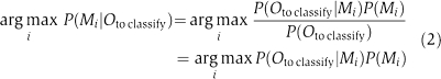
where i=male or female.

In this study, HMMs were compared with two linear classification methods: LDA (Ripley, 1996) and partial least squares (PLS) regression (Hastie et al, 2001). LDA is a statistical technique used to find the linear combination of the features (here, metabolite concentrations) giving the best separation between the classes (here, males and females). The LDA classification rule is

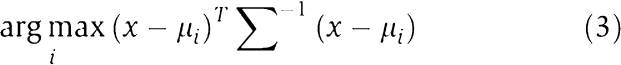
where x is a vector to be classified, μ_i is the mean vector of class i (male or female) and Σ is the covariance matrix (assumed to be shared by both classes). We estimated the covariance matrix from the pooled set of all time points. LDA does not have complexity parameters analogous to HMM states that should be optimized; it was thus fast to compute.

The second classification method, PLS, is a linear regression method that extends and combines properties of multiple regression and principal component analysis. It is especially useful when the number of predictors is large compared with the number of observations. The purpose of PLS is to predict the class y (here, males/females, transformed to 0/1) with the feature matrix X (here, time series data O broken down to single observations). PLS searches for a set of components that performs a simultaneous decomposition of X and y, with the constraint that the components should explain as much of the covariance between X and y as possible. The actual PLS-DA, in other words the classification, can then be performed by discretizing the continuous prediction given by PLS regression to 0 or 1, corresponding to boys and girls, respectively. The number of components in PLS was not of primary interest here, and it was thus optimized with cross-validation for each bootstrap sample and then the out-of-bag samples were classified with PLS-DA based on the discovered, optimal set of latent components.

Supplementary Material

Supplementary Material

Supplementary Information 1

Supplementary Information 2

References

- Efron B (1994) An Introduction to Bootstrap. New York: Chapman & Hall [Google Scholar]
- Fahy E, Subramaniam S, Brown HA, Glass CK, Merrill AH Jr, Murphy RC, Raetz CRH, Russell DW, Seyama Y, Shaw W, Shimizu T, Spener F, van Meer G, VanNieuwenhze MS, White SH, Witztum JL, Dennis EA (2005) A comprehensive classification system for lipids. J Lipid Res 46: 839–862 [DOI] [PubMed] [Google Scholar]
- Hastie T, Tibshirani R, Friedman JH (2001) The Elements of Statistical Learning: Data Mining, Inference, and Prediction. New York: Springer Verlag [Google Scholar]
- Jansen JJ, Hoefsloot HCJ, Boelens HFM, van der Greef J, Smilde AK (2004) Analysis of longitudinal metabolomics data. Bioinformatics 20: 2438–2446 [DOI] [PubMed] [Google Scholar]
- Katajamaa M, Miettinen J, Oresic M (2006) MZmine: toolbox for processing and visualization of mass spectrometry based molecular profile data. Bioinformatics 22: 634–636 [DOI] [PubMed] [Google Scholar]
- Kell DB (2006) Metabolomics, modelling and machine learning in systems biology—towards an understanding of the languages of cells. Delivered on 3 July 2005 at the 30th FEBS Congress and 9th IUBMB conference in Budapest. FEBS J 273: 873–894 [DOI] [PubMed] [Google Scholar]
- Kriete A, Sokhansanj BA, Coppock DL, West GB (2006) Systems approaches to the networks of aging. Ageing Res Rev 5: 434–448 [DOI] [PubMed] [Google Scholar]
- Kupila A, Keskinen P, Simell T, Erkkilä S, Arvilommi P, Korhonen S, Kimpimäki T, Sjöroos M, Ronkainen M, Ilonen J, Knip M, Simell O (2002) Genetic risk determines the emergence of diabetes-associated autoantibodies in young children. Diabetes 51: 646–651 [DOI] [PubMed] [Google Scholar]
- Kupila A, Muona P, Simell T, Arvilommi P, Savolainen H, Hämäläinen A-M, Korhonen S, Kimpimäki T, Sjåroos M, Ilonen J, Knip M, Simell O (2001) Feasibility of genetic and immunological prediction of type 1 diabetes in a population-based birth cohort. Diabetologia 44: 290–297 [DOI] [PubMed] [Google Scholar]
- Laaksonen R, Katajamaa M, Päivä H, Sysi-Aho M, Saarinen L, Junni P, Lütjohann D, Smet J, Coster RV, Seppänen-Laakso T, Lehtimäki T, Soini J, Oresic M (2006) A systems biology strategy reveals biological pathways and plasma biomarker candidates for potentially toxic statin induced changes in muscle. PLoS ONE 1: e97. [DOI] [PMC free article] [PubMed] [Google Scholar]
- Lenz EM, Bright J, Wilson ID, Hughes A, Morrisson J, Lindberg H, Lockton A (2004) Metabonomics, dietary influences and cultural differences: a 1H NMR-based study of urine samples obtained from healthy British and Swedish subjects. J Pharm Biomed Anal 36: 841–849 [DOI] [PubMed] [Google Scholar]
- Mehta D (2005) Lysophosphatidylcholine: an enigmatic lysolipid. Am J Physiol Lung Cell Mol Physiol 289: L174–L175 [DOI] [PubMed] [Google Scholar]
- Merrill A, Wang E, Innis W, Mullins R (1985) Increases in serum sphingomyelin by 17{beta}-estradiol. Lipids 20: 252–254 [DOI] [PubMed] [Google Scholar]
- Murphy K (1998) Hidden Markov Model (HMM) Toolbox for Matlab, http://www.cs.ubc.ca/~murphyk /Software/HMM/hmm.html accessed November 6, 2007 [Google Scholar]
- Nicholson JK, Holmes E (2006) Global systems biology and personalized healthcare solutions. Discov Med 6: 63–70 [PubMed] [Google Scholar]
- Nicholson JK, Holmes E, Wilson ID (2005) Gut microorganisms, mammalian metabolism and personalized health care. Nat Rev Microbiol 3: 431–438 [DOI] [PubMed] [Google Scholar]
- Oresic M, Vidal-Puig A, Hänninen V (2006) Metabolomic approaches to phenotype characterization and applications to complex diseases. Expert Rev Mol Diagn 6: 575–585 [DOI] [PubMed] [Google Scholar]
- Rabiner L (1989) A tutorial on hidden Markov models and selected applications in speech recognition. Proc IEEE 77: 257–286 [Google Scholar]
- Rezzi S, Ramadan Z, Martin F-PJ, Fay LB, vanBladeren P, Lindon JC, Nicholson JK, Kochhar S (2007) Human metabolic phenotypes link directly to specific dietary preferences in healthy individuals. J Proteome Res 6: 4469–4477 [DOI] [PubMed] [Google Scholar]
- Ripley BD (1996) Pattern Recognition and Neural Networks. Cambridge, UK: Cambridge University Press [Google Scholar]
- Smilde AK, Jansen JJ, Hoefsloot HCJ, Lamers R-JAN, van der Greef J, Timmerman ME (2005) ANOVA-simultaneous component analysis (ASCA): a new tool for analyzing designed metabolomics data. Bioinformatics 21: 3043–3048 [DOI] [PubMed] [Google Scholar]
- ‘t Hart BA, Vogels JTWE, Spijksma G, Brok HPM, Polman C, van der Greef J (2003) 1H-NMR spectroscopy combined with pattern recognition analysis reveals characteristic chemical patterns in urines of MS patients and non-human primates with MS-like disease. J Neurol Sci 212: 21–30 [DOI] [PubMed] [Google Scholar]
- van der Greef J, Stroobant P, Heijden Rvd (2004) The role of analytical sciences in medical systems biology. Curr Opin Chem Biol 8: 559–565 [DOI] [PubMed] [Google Scholar]
- Vance DE, Vance JE (eds) (2004) Biochemistry of Lipids, Lipoproteins and Membranes. The Netherlands: Elsevier BV, Amsterdam [Google Scholar]
- Wang Y, Lawler D, Larson B, Ramadan Z, Kochhar S, Holmes E, Nicholson JK (2007) Metabonomic investigations of aging and caloric restriction in a life-long dog study. J Proteome Res 6: 1846–1854 [DOI] [PubMed] [Google Scholar]
- Yetukuri L, Katajamaa M, Medina-Gomez G, Seppänen-Laakso T, Puig AV, Oresic M (2007) Bioinformatics strategies for lipidomics analysis: characterization of obesity related hepatic steatosis. BMC Syst Biol 1: e12. [DOI] [PMC free article] [PubMed] [Google Scholar]
Associated Data
This section collects any data citations, data availability statements, or supplementary materials included in this article.
Supplementary Materials