Parametric Rietveld refinement

The use of ‘parametric Rietveld refinement’ to extract information from large numbers of powder diffraction patterns using a single evolving structural model is described.

Abstract

In this paper the method of parametric Rietveld refinement is described, in which an ensemble of diffraction data collected as a function of time, temperature, pressure or any other variable are fitted to a single evolving structural model. Parametric refinement offers a number of potential benefits over independent or sequential analysis. It can lead to higher precision of refined parameters, offers the possibility of applying physically realistic models during data analysis, allows the refinement of ‘non-crystallographic’ quantities such as temperature or rate constants directly from diffraction data, and can help avoid false minima.

1. Introduction

It is well established that by performing diffraction studies as a function of an external variable (frequently temperature, time, pressure or chemical environment) one can learn more about a system than from a single diffraction experiment. Examples are numerous but include probing structural phase transitions or intermolecular forces, looking at the influence of magnetic or electric fields, or monitoring chemical reactions/transformations. In some cases, it is possible to extract ‘non-crystallographic’ information (i.e. information beyond fractional coordinates, site occupancies and atomic displacement parameters, ADPs) from such measurements. Examples include extracting information about vibrational frequencies (David et al., 1999 ▶) from thermal expansion parameters or ADPs (Bürgi & Capelli, 2000 ▶; Radaelli et al., 1996 ▶), or information such as activation energies or reaction mechanisms from time-dependent studies (David et al., 1993 ▶; Allen & Evans, 2003 ▶, 2004 ▶; Kisi & Riley, 2002 ▶; Evans & Evans, 2004 ▶; Milanesio et al., 2003 ▶; Grizzetti & Artioli, 2002 ▶; Walton & O’Hare, 2000 ▶). Such applications are becoming increasingly widespread, especially in the field of powder diffraction, where the advent of high-intensity sources and area detectors at both central facilities and home laboratories means that extremely rapid high-quality measurements can now be performed (in minutes in a home laboratory or at a neutron source, and in a matter of seconds or less at a synchrotron).

The traditional way to treat data from such studies has been to use Rietveld refinement to analyse individual data sets independently. If, for example, one recorded 100 powder diffraction patterns at different temperatures, each requiring refinement of 20 parameters, one would perform 100 independent refinements using 2000 parameters in total. It is clear, however, that these 2000 parameters are not completely independent. The fractional coordinate of an atom at temperature T will clearly be related (provided that no phase transition occurs) to its coordinate at T ± ΔT. In such a study, one often does not want to determine n parameters at m temperatures, but how the n key parameters evolve with temperature. There are also often parameters which ought to remain unchanged throughout the diffraction experiment. Examples might be the 2θ zero point of a laboratory diffractometer, or the unchanging chemical composition of a sample. If our 100 diffraction patterns were recorded for 1 min each, the uncertainty in a zero-point correction from an individual data set would be large, leading to large uncertainties in other parameters; if, however, one could derive this quantity from all 100 patterns collected for 100 min simultaneously, its uncertainty would be considerably reduced.

In this paper we describe a general methodology for addressing this issue in which any parameter can be described by a single overall value or by a function describing its evolution throughout the data collection, and can be simultaneously refined from a large body of diffraction data. For convenience we call this approach ‘parametric Rietveld refinement’ to emphasize that one parametrically fits a three-dimensional surface of 2θ, intensity and temperature (or time, pressure, etc.) space. This approach offers potential benefits over sequential analysis: it can significantly reduce correlations between parameters and reduce final standard uncertainties; it can allow one to introduce simple physically meaningful constraints or restraints to a refinement; it can help one avoid false minima with low-quality individual data sets; and it can allow the direct refinement of ‘non-crystallographic’ parameters such as temperature and rate constants from diffraction data. §2 of this paper will outline the philosophy/methodology of the approach. §3 contains information on calibration materials used for the examples described. §4 describes three applications: the use of parametric refinement to reduce uncertainties in cell-parameter determination; the use of internal standards to refine the true experimental temperature of a sample from diffraction data; and the use of parametric fitting to extract kinetic information.

The philosophy behind the method is, of course, similar to the use of multiple data sets across an X-ray absorption edge, multiple banks of a time-of-flight neutron data set or combined neutron and X-ray data sets to improve structural precision. Limited linking of parameters between data sets for such applications is available in several Rietveld codes but, to the best of our knowledge, the only previous implementation of constraint equations is in the XND code, which allows the use of simple polynomials for selected variables (Berar & Baldinozzi, 1998 ▶). The method we describe is, however, entirely general, extremely flexible and can be used in a wide variety of situations. We note that the mind-set to adopt when applying this approach is similar to that when using restraints or constraints in other areas of crystallography. One must ensure that the ‘extra information’ one introduces during the refinement is appropriate, otherwise the derived parameters will be detrimentally affected.

2. Methodology

All parametric refinements reported here have been performed using the TOPAS-Academic software written by Alan Coelho (Coelho, 2000a ▶). One significant aspect of this software is that it supports user-defined equations in an entirely general way such that highly sophisticated/specialized models can be introduced without access to the source code. The software is also fast, robust and can handle an essentially unlimited number of parameters.

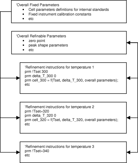
The general form of an input file used for parametric fitting is shown schematically in Fig. 1 ▶ for a variable temperature experiment. A typical control file (for a case such as example 2 below) has been deposited as supplementary information.1 The file contains a series of sections (one per temperature) which contain instructions required to perform Rietveld refinement of each individual data set. Individual variables within these blocks can be assigned convenient names. In a variable-temperature experiment, one might assign names such as a_t0300 or x_C1_t0300 to the a cell parameter and x fractional coordinate of atom C1 at 300 K, respectively. Simple instructions also allow the values of selected parameters to be output to a text file after refinement. There are then two sections which describe ‘overall’ parameters which apply to all the data sets. These are separated for convenience into ‘fixed’ and ‘refinable’ paramaters. The diffractometer zero point, for example, could be defined as a single overall refinable parameter (zero_overall) and fed into each data set using equation (1):

Most equations quoted use the TOPAS format, which is defined elsewhere (Coelho, 2006 ▶); briefly, where a defined parameter (prm) has a name preceded by ‘!’, it is a fixed quantity; otherwise it is free to refine. Other variables might be expected to show a simple dependence on temperature. For example, it is frequently found that the sample height in a high-temperature laboratory Bragg–Brentano experiment varies linearly with temperature due to thermal expansion of the furnace. One would then describe the sample height at each set temperature (e.g. Tset = 300) by an expression such as equation (2):

where c1 and c2 are overall parameters refined from all the data. This quantity would then be used to apply a correction of the form described to the 2θ values of the calculated data at each experimental temperature. Similar equations can be introduced to apply a variety of 2θ corrections for different experimental factors.

Figure 1.

Schematic layout of an input file used for parametric Rietveld refinement.

In some situations (see below) one might wish to impose known physical behaviour during a refinement. In example 2, we apply the known thermal expansion of calibration materials during multi-phase Rietveld refinement. This is done in the overall fixed variables section. For example, cell parameters can frequently be accurately described by an expression such as equation (3) over wide temperature ranges (Reeber, 1975 ▶; Wang & Reeber, 2000 ▶):

where a ₀ is the cell parameter at 0 K, an Einstein temperature and c _n an empirically derived coefficient. In TOPAS this can be expressed by defining a ₀, c _n and as fixed values in the overall section of the input file and passing this information into each individual data set. The relevant format would be:

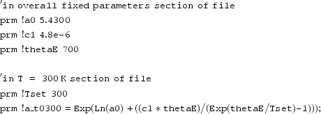As described in more detail in example 2, this offers the possibility of refining a ‘non-crystallographic’ parameter from diffraction data. If the cell parameter forced on the refinement by the prescribed equation (here !a_t0300) does not match the experimental peak positions due to a discrepancy between the furnace set temperature (Tset) and the true sample temperature, one can introduce a refinable parameter delta_t0300 to accommodate this. The relevant section of the input file would become:

The constraint equations described above are entirely general: they can be applied to any refinable quantity (coordinates, occupancies, ADPs, etc.) and can be expressed in terms of any external variable. It would also be possible to restrain (rather than constrain) fitting via parametric equations which apply a penalty of the form (actual_value− ideal_value)² with ideal values defined from all data by simple equations, though this approach has not been explored in this work. To reduce correlations, equations are often expressed with temperature or other quantities rescaled onto a −1 to +1 scale using T* = [T − 0.5(T _MAX + T _MIN)]/(T _MAX − T _MIN) during refinement.

To check that refinements converge to a global minimum, it is possible to adopt a simple simulated annealing approach in which refined quantities are displaced by random amounts (scaled by a ‘temperature’) at convergence and the data re-refined, with the best R-factor solution being retained (Coelho, 2000b ▶). Refinements can also be performed from a variety of random starting positions. All refinements reported here were initially performed using a ‘normal’ sequential independent refinement strategy to provide benchmark values of parameters and agreement factors. For these individual refinements, all parameters in the control file were named according to a ‘_t0000’ convention. A local Fortran routine then automatically replaces this label with one specific for each temperature, allowing input files for parametric refinement to be generated rapidly. Temperatures are extracted automatically, either from data file headers or from experiment log files. Input files also included instructions to produce text files of all refined parameters and their standard uncertainties.

All powder diffraction data reported here were recorded using a Bruker d8 advance diffractometer equipped with a Cu tube, Ge(111) incident-beam monochromator and Vantec or Braun linear PSD (position-sensitive detector). High-temperature measurements were performed using an Anton-Paar HTK1200 furnace. Low-temperature measurements were recorded using an Oxford Cryosystems pHeniX cryostat. For furnace measurements, the sample was ramped to temperature and held at constant temperature throughout the diffraction experiment; in the cryostat the temperature was ramped continuously and a single average temperature determined for each diffraction pattern from experimental log files.

3. Non-ambient internal standards

Two examples of parametric refinement in this paper relate to the determination of accurate and precise cell parameters of materials as a function of temperature. Obtaining accurate (as opposed to precise) non-ambient cell parameters from laboratory Bragg–Brentano data is not trivial. Peak 2θ positions and therefore cell parameters are influenced by a number of sample and instrumental factors, including sample height, sample absorption, instrumental calibration, the peak shape model used and the experimental temperature (Klug & Alexander, 1974 ▶; Pecharsky & Zavilij, 2003 ▶; Beck & Mittemeijer, 2002 ▶). It is standard practice to correct for the first four of these effects using an internal standard such as NIST 640c silicon, which has a = 5.4311946 Å at 295.65 K (NIST, 2000 ▶) For variable-temperature work, it is necessary to know the temperature dependence of the cell parameters. For Si we have taken thermal expansion data from 6 to 340 K provided by Lyon et al. and from 300 to 1500 K by Okada et al. (Lyon et al., 1977 ▶; Okada & Tokumaru, 1984 ▶). Data were normalized to fit the NIST 296.5 K cell value. We find that the experimental data can be accurately described over the whole temperature range by equation (3) with coefficients given in Table 1 ▶, with the maximum discrepancy between fitted and expansion-derived cell parameters being <5 × 10⁻⁵ Å over the entire temperature range.

Table 1. Coefficients used to describe the temperature dependence of the cell parameter of Si using equation (3) .

a0	5.42999 Å
c1/θ1	−1.270 × 10−6	217 K
c2/θ2	4.815 × 10−6	571 K
c3/θ3	1.019 × 10−6	1500 K

In the case of Al₂O₃, thermal expansion data have been collated by Toulakien and by Taylor (Taylor, 1984 ▶; Toulakian et al., 1977 ▶). We have chosen to take Taylor’s expression for the temperature dependence of cell parameters [equation (4)]. The x ₀ values quoted differ from those of Taylor but yield cell parameters at 295 K consistent with those reported by Cline for NIST SRM676 (NIST, 1991 ▶). Note that Taylor’s expression uses temperature in °C not K:

For non-ambient work, if the thermal expansion of the internal standard were precisely known, it could be used to calibrate experimental temperature (see below). This process can, however, be prone to significant errors since a small systematic error in cell parameter can lead to a large error in temperature determination. For this reason, we prefer to employ two internal standards at high temperature; one with low expansion (e.g. Si) and one with high (e.g. Al₂O₃). Since systematic errors in cell determination of each standard will be similar, one can use the differential thermal expansion to determine temperature (Fig. 2 ▶ c); the ratio of cell volumes, or difference in the two curves of Fig. 2 ▶(c), providing a direct measure of temperature.

Figure 2.

Temperature dependence of (a) Si cell parameter [open diamonds derived from experimental dilatometry data; solid line from equation (3)] and (b) Al₂O₃ cell parameters (solid lines) used in this work. (c) The difference in thermal expansion, here plotted as V(T)/V(293.15 K), allows a direct measure of temperature.

4. Examples

4.1. Example 1 – improving precision of cell parameter determination

This example shows that by treating data as an evolving ensemble using parametric refinement and internal standards, it is possible to obtain accurate values of cell parameters and to improve the precision with which they can be determined.

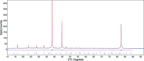
Rb[MnCr(CN)₆].xH₂O is one of a large family of Prussian Blue related materials. Many of these have been shown to undergo structural and/or magnetic/electronic transitions as a function of temperature, which are frequently manifested in the thermal expansion of the material (Chapman et al., 2006 ▶; Margadonna et al., 2004a ▶,b ▶). As part of a series of experiments (Prassides, 2006 ▶), diffraction data were collected on this material on cooling from 293 K to 16 K at a cooling rate of 8 K h⁻¹ using a pHeniX cryostat. Data were collected in ∼40 min time slices over a 10–90° 2θ range corresponding to a data set every ∼5 K. Average cryostat temperatures for each data set were extracted from a log of the experimental temperature with time. To obtain reliable cell parameters, the sample was mixed with Si before being sprinkled as a thin layer on an Al plate. Due to the small amount of sample available and its relatively low absorption, significant peaks due to the sample holder are present in the diffraction pattern (Fig. 3 ▶). Extracting reliable cell parameters from the relatively weak sample peaks is therefore challenging.

Figure 3.

Rietveld refinement of an Rb[MnCr(CN)₆].xH₂O/Si mixture recorded at 16 K. Observed data are in red, calculated in blue. The strong peaks at ∼38, ∼45 and ∼83° 2θ are due to the Al sample holder and fitted using the Pawley method (note that the data are presented on an scale to emphasize the weak sample peaks). The lowest tick marks are Al peaks, the middle tick marks are for the sample, and the upper tick marks the Si internal standard.

In this experiment, the key factors to consider when determining sample cell parameters are the calibration of the diffractometer (zero points, PSD calibration, etc.) and the sample height which will vary with temperature due to thermal expansion of the cryostat. If the Al peaks are to be fitted during sample cell determination (which gives an independent estimate of the true cryostat temperature) it should be remembered that the mounting method means that the effective sample height will be offset slightly from the effective height of the Al holder surface.

Initially we adopted a traditional approach to data analysis in which individual patterns were analysed separately. We selected a single T = 16 K data set and performed a three-phase refinement in which the sample and Si diffraction were fitted by the Rietveld method and peaks of the Al sample holder by the Pawley method (due to texture affecting intensities). Scale factors and peak shape parameters were refined for each phase along with background terms. For Al and Rb[MnCr(CN)₆].xH₂O, the cubic cell parameter was allowed to refine along with a height correction for both Al and the sample (Si and sample heights were equated). The Si cell parameter was fixed at 5.42999 Å and a 2θ calibration was applied by refining coefficients of a second-order polynomial. Polynomial coefficients were then fixed at 16 K derived values and this model used to refine all subsequent temperatures independently (44 parameters refined for 64 independent data sets = 2816 parameters in total). R _wp values for individual refinements ranged from ∼9.2 to ∼8.6% with an average value of 8.914%.

An alternative protocol is to realise that several variables in this experiment will, to a good approximation, remain unchanged or vary smoothly during the course of the experiment. In particular, the 2θ calibration polynomial and the height offset between the sample and sample holder should remain unchanged; overall sample/sample holder heights should vary smoothly. These parameters are therefore better derived from the entire 42 h data ensemble than from a single 40 min data set. To allow this, an equivalent parametric refinement protocol was therefore followed to that used for independent refinements.

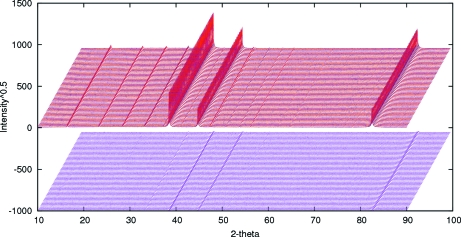
In an initial round of parametric refinement, the Si cell parameter was expressed as a fixed quantity in terms of equation (3) and a 2θ correction polynomial and sample height offset refined from all 64 data sets simultaneously; parameters describing an overall pseudo-Voigt peak shape were also refined for each phase. In this process, a total of 1747 parameters were refined (19 overall parameters: 3 terms of a calibration polynomial, a height offset between sample and holder and 5 overall peak shape parameters per phase; 27 parameters per individual data set: 15 background terms, 2 scale factors, 2 cell parameters, an isotropic overall temperature factor for Si and the sample, 5 hkl peak intensities for the Al Pawley fit, and the sample height of the Al holder). Coefficients of the 2θ calibration polynomial were then fixed and parametric Rietveld refinement performed using a single parameter to describe the sample height offset and with the Si cell allowed to refine freely. An overall R _wp of 9.05% was obtained with higher temperature refinements showing slightly worse agreement factors than for free refinements. Allowing Al peak shapes for each data set to refine independently led to an overall R _wp = 8.925%, individual R _wp values for each data set that varied smoothly with temperature, and smooth changes in peaks shape values; these minor variations are presumably caused by small changes in sample height with temperature. The parametric R factor is essentially the same as the average of those obtained by independent refinements. Fig. 4 ▶ shows the equivalent of a standard Rietveld plot for the parametric refinement.

Figure 4.

Parametric Rietveld refinement of Rb[MnCr(CN)₆].xH₂O. Observed data in are red, calculated in blue. Data have been offset in 2θ and intensity for clarity. The difference surface is plotted in pink.

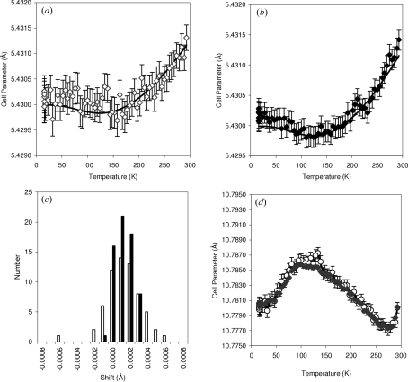
Fig. 5 ▶ shows the Si and sample cell parameters obtained by this protocol compared with free refinements. While the overall trends in behaviour are comparable, the scatter on data points from parametric fitting is considerably lower than from independent refinements. Average standard uncertainties on Si cell parameters are 0.00028 Å from individual refinements and 0.00017 Å from parametric fitting; for the sample values are 0.0008 Å and 0.0003 Å, respectively. The significantly narrower spread of values is also shown in Fig. 5 ▶(c), which shows deviations of refined values from those of equation (3) for the two refinements.

Figure 5.

(a) The Si cell parameter from independent refinement of data sets and (b) from parametric fitting. In each case the solid line represents equation (3). (c) A histogram of the offset between refined and ideal Si cell parameters. (d) Superposition of the sample cell parameter obtained by the two methods. In each graph, open symbols represent independent fitting, and closed symbols represent parametric fitting. For ease of comparison, both individual and parametric fitting refinement values used the 2θ correction polynomial derived from parametric fitting.

The increased precision in cell determination can be traced to the precision with which the true sample height is determined. For free individual refinements, the offset between the (well determined) Al height and that of the sample had an average of 0.025 (2) mm (the standard deviation of all 64 values refined being 0.002 mm; the average Rietveld-derived standard uncertainty was 0.003 mm); from parametric fitting the overall value was 0.0247 (3) mm. The precision to which the sample height is determined is thus improved by an order of magnitude by parametric fitting. In essence, one is using the assumption of a constant offset between sample and sample holder to transfer the precision of Al height determination (∼0.0003 mm) to the sample. The true accuracy of height determination is, of course, much lower due to correlation with instrumental calibration constants. We note that alternative parameterization strategies are possible in the parametric fitting approach. One can, for example, reduce the number of parameters by describing the Al and/or sample height as a simple function of temperature, e.g. three coefficients of a polynomial function to describe height replacing 64 independent parameters. For these data, using parameterized Al and sample heights in this way gives an overall R _wp of 8.927%, essentially unchanged from that using unconstrained heights. The height offset between the sample and Al varied by less than 0.002 mm between 16 and 293 K. The precision and values of refined cell parameters were essentially unchanged using this model. This alternative approach thus validates the assumption of an insignificant change in sample offset from sample holder with temperature.

4.2. Example 2 – refining ‘non-crystallographic’ parameters

ZrP₂O₇ is a material that has attracted attention for its unusual thermal expansion properties. At room temperature, it has been shown by ³¹P NMR and diffraction to have a 3 × 3 × 3 pseudo-cubic orthorhombic structure (related to a simple 1 × 1 × 1 cubic aristotype) containing a remarkable 136 crystallographically unique atoms (King et al., 2001 ▶; Stinton et al., 2006 ▶; Birkedal et al., 2006 ▶). On heating, the material undergoes a phase transition to the simple cubic structure with a phase transition temperature of 567 K determined by differential scanning calorimetry (DSC). To understand the origins of the low and even negative thermal expansion behaviour in the wider AM ₂O₇ family of materials (Evans et al., 1998 ▶), an accurate measure of the temperature dependence of unit-cell parameters is necessary.

Variable-temperature powder diffraction data were recorded on a sample of ZrP₂O₇ [the synthesis of which has been described elsewhere (Stinton et al., 2006 ▶)], mixed and ground with equal masses of Si and Al₂O₃. 51 data sets were recorded from 303 to 677 K on warming and cooling. A slow N₂ flow was passed over the sample during measurements. In an initial round of analysis, each data set was Rietveld refined independently using a simple cubic structural model for ZrP₂O₇. At each temperature, a total of 53 parameters were refined: 4 cell parameters (1 ZrP₂O₇, 1 Si, 2 for Al₂O₃), the sample height, 3 scale factors, 18 background parameters, 6 peak shape parameters per phase, a peak asymmetry correction, 7 isotropic displacement parameters (1 Zr, 1P, 2*O for ZrP₂O₇; 1 for Si; 1 for Al and 1 for O of Al₂O₃) and a P fractional coordinate. Calibration of the 2θ scale was performed using the Si internal standard by application of a second order correction polynomial as described above with coefficients determined from a 16 h data collection performed immediately before the variable-temperature runs and with values fixed for subsequent refinements. Individual R _wp values varied smoothly with temperature from 18.13 to 19.94% with an average of 18.94%.

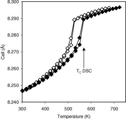
The key quantity from these independent refinements, the pseudo-cubic cell of ZrP₂O₇, is shown in Fig. 6 ▶. Whilst the phase transition from the 3 × 3 × 3 orthorhombic to the 1 × 1 × 1 cubic structure is clearly visible, the phase transition temperature (512–527 K) is significantly lower than found by calorimetry (567 K). However, significant discrepancies are also observed between the expected and observed temperature dependence of cell parameters of the internal standards.

Figure 6.

Cell parameter of ZrP₂O₇ derived from independent refinements (open symbols) and parametric fitting using a polynomial temperature correction (closed symbols). Data are plotted against the furnace set temperature and Rietveld-refined temperature, respectively.

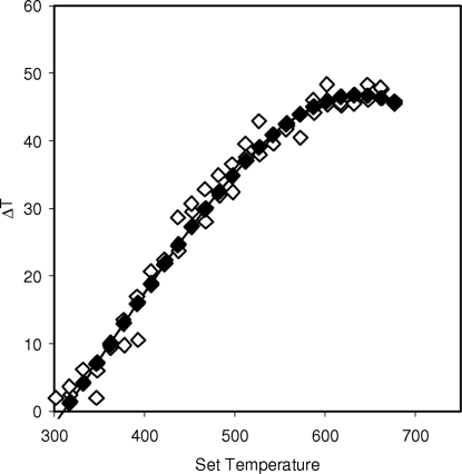
In order to determine the true sample temperature from the diffraction data, we have adopted a parametric fitting approach. Two methods have been used. In the first, instead of refining the cell parameters of the internal standards for each individual data set, they have been defined in terms of equations (3) and (4) using the coefficients of Tables 1 ▶ and 2 ▶. For each data set, a ΔT temperature offset was introduced and refined as described in §2. This allows one to minimize the discrepancies between the observed and calculated peak positions of the internal standards. A total of 2501 parameters were refined to fit simultaneously all 50 data sets. An overall R _wp of 18.88% was achieved, similar to the average R _wp for independent refinements. A plot of the temperature offset refined from the diffraction data is shown in Fig. 7 ▶. One might expect that the temperature gradients leading to discrepancies between actual and set temperatures in the furnace would vary smoothly with set temperature. It is therefore possible to fit with fewer parameters by defining a ΔT correction polynomial of the form ΔT = c ₀ + c ₁ T + c ₂ T ², where c ₀, c ₁ and c ₂ are parameters refined simultaneously from the whole data set. Fitting using this second approach gave an overall R _wp of 18.89%. The ΔT calibration curve obtained is shown in Fig. 7 ▶. Cell parameters plotted against the Rietveld-refined temperature are shown in Fig. 6 ▶. The diffraction-derived phase transition temperature lies between T = 550 and T = 567 K, in much better agreement with the DSC data.

Table 2. Coefficients used to describe the temperature dependence of the cell parameter of Al₂O₃ using equation (4) (note that this equation uses temperature in °C).

	a	c
c0	4.75814 Å	12.99113 Å
c1	6.55 × 10−6	6.54 × 10−6
c2	1.82 × 10−9	2.60 × 10−9

Figure 7.

The difference between experimental and actual sample temperatures as derived by parametric Rietveld refinement. Open symbols are ΔT values refined independently from each data set; closed symbols are the ΔT polynomial refined from all data simultaneously.

Clearly the temperature steps in this experiment are too coarse to define T _C to closer than ±15 K. To see how far our parametric fitting ideas can be pushed, we have collected 871 data sets for 4.75 min each in 2 K steps from 303 to 1173 K. Each data set contains a total of 4997 data points from 5 to 90° 2θ (step size 0.017°). Fig. 8 ▶ shows the results obtained on analysing the data by two protocols. Fig. 8 ▶(a) shows results from independent refinement of each data set (53 parameters at 871 temperatures or 46163 parameters in total for independent refinements) using a protocol similar to that described above. There is significant scatter in the resulting parameters, particularly in temperatures refined from an individual data set, but the general shape of the temperature dependence of the refined cell parameter is reasonable. Fig. 8 ▶(b) shows the results of parametric fitting of the same data using a ΔT polynomial derived from all data simultaneously. Using a 3 GHz desktop PC with 2 Gbyte of RAM, all 871 data sets could only be refined on a realistic time scale by rebinning the step size and we therefore chose to refine every second data set. This requires a total of 13507 parameters (cf. a total of 23055 for equivalent independent refinements). Even when fitting 435 data sets simultaneously, each cycle of refinement took ∼1.5 min on a 3 GHz desktop PC, and convergence was achieved within <25 cycles. A considerable reduction in the cell parameter scatter is achieved and the refined phase transition temperature is between 567 and 571 K, close to the DSC value of 567 K. The refined ΔT polynomial is very similar to that of Fig. 7 ▶ over the temperature range of overlap.

Figure 8.

Cell parameters from (a) independent and (b) parametric fitting of 871 and 435 data sets; closed points, warming; open points, cooling. (c) The region close to the phase transition. Data taken on warming are represented by squares; cooling data by circles; open symbols represent independent fitting; closed symbols represent parametric fitting.

4.3. Example 3 – kinetic refinements

The cubic AM ₂O₈ (A = Zr, Hf; M = W, Mo) family of materials display two unusual structural properties: they show negative thermal expansion over a wide temperature range (Evans et al., 1999 ▶, 1996 ▶, 2000 ▶; Mary et al., 1996 ▶) and undergo an order–disorder transition at relatively low temperatures (450 K for ZrW₂O₈, 270 K for ZrWMoO₈) which is associated with the onset of oxygen mobility (Hampson et al., 2005 ▶, 2004 ▶; Allen & Evans, 2004 ▶, 2003 ▶). We have previously described how the high-temperature β phase of ZrWMoO₈ can be quenched to low temperature; powder diffraction measurements as a function of time then allow the kinetics of the β (high temperature, oxygen disordered) to α (low temperature, oxygen ordered) phase to be followed by powder diffraction (Allen & Evans, 2004 ▶). The kinetics of oxygen mobility are revealed by the diffraction data in two ways. Firstly, the fractional occupancies of certain sites change on ordering and the material changes symmetry from Pa (β) to P2₁3 (α). The kinetics can then be followed from the intensity of 0kl, k ≠ 2n, reflections, forbidden in the β phase but present in α, or via Rietveld refinement of site occupancies. Secondly, there is a small positive volume change associated with the oxygen ordering such that kinetic information can be extracted from unit-cell parameter changes.

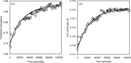
Previously (Allen & Evans, 2004 ▶) we have reported a kinetic study of this system in which a series of isothermal diffraction data were refined independently and kinetic information extracted from the resultant structural models. Fig. 9 ▶(a) shows the key fractional occupancy and Fig. 9 ▶(b) the unit-cell parameter as a function of time extracted from 97 powder patterns recorded over a period of 29 h at 215 K. Each individual data set was independently fitted by Rietveld refinement using a total of 32 parameters, implying 3104 parameters in total (1 cell, 1 scale factor, a sample height, 6 terms to describe a pseudo-Voigt peak shape function, 2 terms to describe additional broadening of 0kl reflections, 9 background terms, 11 fractional coordinates and a fractional occupancy). The average R _wp for all refinements was 29.007%.

Figure 9.

(a) Fractional site occupancy and (b) unit-cell parameters extracted from independent Rietveld refinements (open symbols) and by parametric fitting (solid line).

Using parametric Rietveld methodology, the same data can be fitted simultaneously. To achieve this, a single overall structural model was used and fractional occupancies and cell parameters were described during parametric refinement by the expressions

and

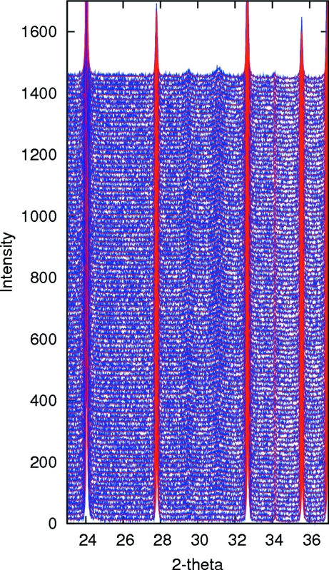
where k _frac and k _cell are rate constants for the change in fractional occupancy, t is time, and c _n are refinable parameters. All 97 data sets were then fitted with a total of 1860 parameters (11 overall structural parameters and 6 rate expression coefficients; 97 times 19 peak shape, scale factor, height and background parameters per data set). An overall set of fractional coordinates is appropriate for this case; for more complex systems fractional coordinates could also be parameterized. An overall R _wp of 28.833% was achieved; the kinetic Rietveld fit is shown in Fig. 10 ▶. The lower R _wp value compared with free refinements is due to individual free refinements becoming stuck in false local minima which are avoided by the use of a single overall structural model in the parametric refinement. Rietveld-refined rate expressions obtained are superimposed on data from independent refinements in Figs. 9 ▶(a) and 9 ▶(b). Rietveld refined rate constants of k _frac = 3.9 (2) × 10⁻⁵ and k _cell = 3.7 (2) × 10⁻⁵ s⁻¹ were obtained, suggesting that both peak intensity and cell parameters yield essentially equivalent kinetic data.

Figure 10.

Kinetic parametric Rietveld fit. Peaks appearing at ∼29 and ∼31° 2θ show the α to β transition.

5. Conclusions

We have shown that parametric fitting can have significant advantages over sequential fitting of parametric data sets. Firstly, data can be fitted using fewer free variables. Secondly, it is possible to use the entire data set to determine certain parameters which can reduce derived uncertainties and help avoid false minima. Thirdly, it is possible to reduce the standard uncertainties in parameters that would be significantly correlated from data collected at a single temperature. Finally, it becomes possible to refine non-crystallographic quantities such as experimental temperature and rate constants for kinetic processes directly from diffraction data.

References

- Allen, S. & Evans, J. S. O. (2003). Phys. Rev. B, 68, 134101–134103.
- Allen, S. & Evans, J. S. O. (2004). J. Mater. Chem.14, 151–156.
- Beck, M. & Mittemeijer, E. J. (2002). J. Appl. Cryst.35, 103–107. [Google Scholar]
- Berar, J.-F. & Baldinozzi, G. (1998). IUCr–CPD Newslett.20, 3–5.
- Birkedal, H., Andersen, A. M. K., Arakcheeva, A., Chapuis, G., Norby, P. & Pattison, P. (2006). Inorg. Chem.45, 4346–4351. [DOI] [PubMed] [Google Scholar]
- Bürgi, H. B. & Capelli, S. C. (2000). Acta Cryst. A56, 403–412. [DOI] [PubMed] [Google Scholar]
- Chapman, K. W., Chupas, P. J. & Kepert, C. J. (2006). J. Am. Chem. Soc.128, 7009–7014. [DOI] [PubMed] [Google Scholar]
- Coelho, A. A. (2000a). TOPAS, v2.0. Bruker AXS.
- Coelho, A. A. (2000b). J. Appl. Cryst.33, 899–908. [Google Scholar]
- Coelho, A. A. (2006). Topas: Technical Reference, http://members.optusnet.com.au/~alancoelho/.
- David, W. I. F., Evans, J. S. O. & Sleight, A. W. (1999). Europhys. Lett.46, 661–666.
- David, W. I. F., Ibberson, R. M. & Matsuo, T. (1993). Proc. R. Soc. London A, 442, 129–146.
- Evans, J. S. O., David, W. I. F. & Sleight, A. W. (1999). Acta Cryst. B55, 333–340. [DOI] [PubMed] [Google Scholar]
- Evans, J. S. O. & Evans, I. R. (2004). Chem. Soc. Rev.33, 539–547. [Google Scholar]
- Evans, J. S. O., Hanson, P. A., Ibberson, R. M., Duan, N., Kameswari, U. & Sleight, A. W. (2000). J. Am. Chem. Soc.122, 8694–8699.
- Evans, J. S. O., Mary, T. A. & Sleight, A. W. (1998). Physica B, 241, 311–316.
- Evans, J. S. O., Mary, T. A., Vogt, T., Subramanian, M. A. & Sleight, A. W. (1996). Chem. Mater.8, 2809–2823.
- Grizzetti, R. & Artioli, G. (2002). Micro. Meso. Mater.54, 105–112.
- Hampson, M. R., Evans, J. S. O. & Hodgkinson, P. (2005). J. Am. Chem. Soc.127, 15175–15181. [DOI] [PubMed] [Google Scholar]
- Hampson, M. R., Hodgkinson, P., Evans, J. S. O., Harris, R. K., King, I. J., Allen, S. & Fayon, F. (2004). Chem. Commun. pp. 392–393. [DOI] [PubMed]
- King, I. J., Fayon, F., Massiot, D., Harris, R. K. & Evans, J. S. O. (2001). Chem. Commun. pp. 1766–1767. [DOI] [PubMed]
- Kisi, E. H. & Riley, D. P. (2002). J. Appl. Cryst.35, 664–668. [Google Scholar]
- Klug, H. P. & Alexander, L. E. (1974). X-ray Diffraction Procedures for Polycrystalline and Amorphous Materials New York: John Wiley.
- Lyon, K. G., Salinger, G. L., Swenson, C. A. & White, G. K. (1977). J. Appl. Phys.48, 865–869.
- Margadonna, S., Prassides, K. & Fitch, A. N. (2004a). Angew. Chem. Int. Ed.43, 6316–6319. [DOI] [PubMed]
- Margadonna, S., Prassides, K. & Fitch, A. N. (2004b). J. Am. Chem. Soc.126, 15390–15391. [DOI] [PubMed] [Google Scholar]
- Mary, T. A., Evans, J. S. O., Vogt, T. & Sleight, A. W. (1996). Science, 272, 90–92.
- Milanesio, M., Artioli, G., Gualtieri, A. F., Palin, L. & Lamberti, C. (2003). J. Am. Chem. Soc.125, 14549–14558. [DOI] [PubMed] [Google Scholar]
- NIST (1991). https://srmors.nist.gov/certificates/view_cert2gif.cfm?certificate=1976.
- NIST (2000). https://srmors.nist.gov/view_cert.cfm?srm=640C.
- Okada, Y. & Tokumaru, Y. (1984). J. Appl. Phys.56, 314–320.
- Pecharsky, V. & Zavilij, P. (2003). Fundamentals of Powder Diffraction and Structural Characterization of Materials Dordrecht: Kluwer.
- Prassides, K. (2006). Unpublished work.
- Radaelli, P. G., Marezio, M., Hwang, H. Y., Cheong, S. W. & Batlogg, B. (1996). Phys. Rev. B, 54, 8992–8995. [DOI] [PubMed]
- Reeber, R. R. (1975). Phys. Status Solidi A, 32, 321.
- Stinton, G. W., Hampson, M. R. & Evans, J. S. O. (2006). Inorg. Chem.45, 4352–4358. [DOI] [PubMed] [Google Scholar]
- Taylor, D. (1984). Br. Ceram. Trans. J.83, 92–98.
- Toulakian, Y. S., Kirby, R. K., Taylor, R. E. & Lee, T. Y. R. (1977). Thermophys. Prop. Matter, 13, 176–185.
- Walton, R. I. & O’Hare, D. (2000). Chem. Commun. pp. 2283–2291.
- Wang, K. & Reeber, R. R. (2000). Appl. Phys. Lett.76, 2203–2204.
Associated Data
This section collects any data citations, data availability statements, or supplementary materials included in this article.
Supplementary Materials
Supplementary material file. DOI: 10.1107/S0021889806043275/db5010sup1.txt
Schematic annotated input file for parametric refinement