

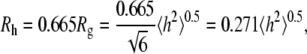
Abstract
A revision (C35r) to the CHARMM ether force field is shown to reproduce experimentally observed conformational populations of dimethoxyethane. Molecular dynamics simulations of 9, 18, 27, and 36-mers of polyethylene oxide (PEO) and 27-mers of polyethylene glycol (PEG) in water based on C35r yield a persistence length λ = 3.7 Å, in quantitative agreement with experimentally obtained values of 3.7 Å for PEO and 3.8 Å for PEG; agreement with experimental values for hydrodynamic radii of comparably sized PEG is also excellent. The exponent υ relating the radius of gyration and molecular weight ( ) of PEO from the simulations equals 0.515 ± 0.023, consistent with experimental observations that low molecular weight PEG behaves as an ideal chain. The shape anisotropy of hydrated PEO is 2.59:1.44:1.00. The dimension of the middle length for each of the polymers nearly equals the hydrodynamic radius
  obtained from diffusion measurements in solution. This explains the correspondence of
  and
and  the pore radius of membrane channels: a polymer such as PEG diffuses with its long axis parallel to the membrane channel, and passes through the channel without substantial distortion.
INTRODUCTION
Polyethylene oxide (PEO) and polyethylene glycol (PEG) are polymers with the subunit C-O-C (Fig. 1). They are well-known encapsulating agents for drug delivery (1), solvents for low temperature crystallography (2–4), and modulators of osmotic pressure (5–8). Low molecular weight PEG readily passes through the pores of membrane proteins (9), and, in fact, can be sized by single channels (10). Comparisons with crystal structures and electron micrographs indicate that the pore radius,  is close to the effective hydrodynamic radius in solution,
  of the largest PEG able to diffuse through the pore or to block ion conductance (11–13). This simple correspondence has allowed estimates of
  for a variety of toxins (11,12,14), porins (13,15), and other ion channels (16,17).
FIGURE 1.

Structures of DME, PEO, and PEG.
The similarity of  and
and  is clearly useful (crystal structures are available for only a small number of membrane proteins), though somewhat surprising. Polymer theory predicts for a random coil polymer in a θ solvent (i.e., an ideal random flight chain) that
 |
(1) |
where  and
and  are the radius of gyration and root mean-squared end-to-end distance, respectively (18). Hence, the average length of the polymer is substantially larger than its hydrodynamic radius. This mismatch raises several possibilities. Theoretical estimates for ideal random chains yield the limiting ratios
  where
where  is the moment of inertia about the ith principal axis, and the brackets signify an average over all conformations (19–22). More recently, the ratio of the lengths of the major and minor axes (or aspect ratio) was determined experimentally for random coil DNA to equal 2.2 (23). These results imply that anisotropy should be considered when modeling the placement of PEG within a pore. It is also possible that the polymer is highly deformed in the pore or that the pore shape is altered by the polymer, so that
  is an accidental surrogate for
  Lastly, the underlying assumptions made in deriving Eq. 1, which include the use of a preaveraged Oseen tensor and neglect of waters of hydration, further confound comparisons.
This study, based on a combination of molecular dynamics (MD) simulations of PEO and PEG in solution and hydrodynamic bead model calculations, examines anisotropy of the shape and translational diffusion tensors of these polymers as a step toward understanding their interaction with membrane pores. The study consists of two parts. The first validates a revision (C35r) of the recently developed CHARMM ether force field (C35) (24). This involved MD simulations of solutions of dimethoxyethane (DME; Fig. 1) and water at different mole fractions, and of 9, 18, 27, and 36-mers of PEO, and 27-mers of PEG in water. The populations of the dominant DME conformations for C35 and C35r are compared with Raman data (25).  for the polymers for the two parameter sets are then shown to have the molecular weight dependence of an ideal chain, as expected from experimental measurements of short length PEG (26,27). This finding enables a determination of the persistence length,
  from each parameter set using the worm-like chain model (18), and a comparison with
  obtained from experiments on high molecular weight PEO (28) and PEG (29).
The second part focuses on the diffusion tensors, hydrodynamic radii, and other measures of polymer shape. It is difficult to obtain unambiguous values of the diffusion constant (and hence  ) from MD simulations of the present systems for two reasons: the statistical error is substantial, and the viscosity of the TIP3P water model (30) must be scaled to compare with experiment (31). Consequently, an alternative estimate of the diffusion constant was obtained using bead model hydrodynamic calculations (32) based on the conformations generated by the MD. The consistency of both approaches lends confidence to the calculated values of
  examination of the assumptions inherent in Eq. 1, and a detailed analysis of the anisotropy.
METHODS
Simulation details
All the simulations and analyses were performed using CHARMM c33b2 (33). Ether parameters were from the CHARMM force field (FF) developed by Vorobyov et al. (C35) (24) and the present revision (C35r), and TIP3P model (30,34) was used for water. Using the new velocity Verlet integrator (35) implemented in CHARMM, the temperature was maintained by applying a Nose-Hoover thermostat (36), and the pressure was maintained at 1 atm by applying an Andersen-Hoover barostat (37,38). Electrostatic forces were evaluated using a particle mesh Ewald (39) summation with κ = 0.34 Å−1, and a real space cutoff of 12 Å; the Lennard-Jones forces were switched to zero between 8 Å and 12 Å, and an isotropic long-range correction (40) was applied. All hydrogen-carbon bond lengths were constrained by SHAKE (41). Simulations were carried out with a time step of 1 fs, and coordinates were saved every picosecond. The parameter and topology files in CHARMM readable format may be obtained from http://mackerell.umaryland.edu/CHARMM_ff_params.html.
Three hundred DME molecules were positioned in a cubic periodic cell of size 38 Å/side and energy minimized by 100 steps of steepest descent (SD) and 500 steps of adopted basis Newton Ralphson (ABNR). Mole fractions of 0.6 and 0.3 were constructed by adding 200 and 700 water molecules, respectively, and each system was energy minimized with 100 steps of SD and 500 steps of ABNR. Six 2 ns trajectories (three for each parameter set) were generated at 318 K, the temperature of the Raman experiment (25), with conformational averages obtained over the last 1 ns; 2 ns simulations of pure DME were also carried out at 298 K to compare with experimental densities, dielectric constant, and heat of vaporization. Gas phase energies at 298 K (necessary for calculating the heat of vaporization) were obtained from 2 ns Langevin dynamics simulations at 298 K.
A fully extended PEO molecule was used as an initial configuration for 9-mers, and the initial configurations for 18, 27, and 36-mers were randomly obtained from the Langevin dynamics simulations at T = 296 K. Two simulations with different initial configurations were performed for each molecular size and force field. The simulated system with 9, 18, or 27-mers consists of a PEO or PEG molecule and ∼2900 water molecules in a periodic box of size 44 Å/side, and the system with 36-mers molecules consists of a PEO molecule and ∼6500 water molecules in a box of dimension 58 Å/side. For each system, the energy was minimized with 30 steps of SD and 100 steps of ABNR. Simulations were performed for 20 ns at 296 K, with averages calculated over the last 18 ns.
Calculation of the persistence length
The persistence length λ was calculated for PEO by a nonlinear least-squares fit (42) of mean-squared end-to-end distance h for the polymer series based on the worm-like chain model (43,44)
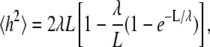 |
(2) |
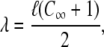
where L is the length of the fully extended polymer. Standard errors for λ were estimated by generating random samples of  based on their statistical errors and refitting. The characteristic ratio
  a commonly reported measure of chain flexibility (45), is related to λ by
 |
(3) |
where  is the geometric mean bond length of the repeating unit, and equals 1.464 Å for PEO (28).
Calculation of the diffusion coefficient from simulation
Diffusion constants from the trajectories  (the subscript denotes periodic boundary conditions) were evaluated from the slopes of the long-time average mean-squared of displacements, MSD(t), of the centers of mass (CM) versus time. As expected for a system consisting of a single solute, MSD(t) was quite irregular at longer times. To improve sampling, the last 18 ns for each simulation was divided into two trajectories of 9 ns, and 4 MSD(t) for each FF, and length of PEO were calculated for 10 ps intervals; these were averaged and a standard deviation
  was calculated for each time point. Displacement of the CM at short times arises from isomerization of dihedral angles, and must be removed when calculating the long-time slope. In this case, the “short-time” cutoff,
  was defined as the statistically independent block size determined for the averaging of
  t0 = 250, 500, 1000, and 2000 ps for the 9, 18, 27, and 36-mers, respectively. Linear regression (42) on the averaged MSD(t) with weighting based on
  was then carried out over the range
  to 5 ns, and the slopes were divided by 6 to obtain
  for each FF and polymer length. The standard deviations of the slopes evaluated for the individual MSD(t) (over the same time intervals and with the same
  ) were used to estimate standard errors for each diffusion constant.
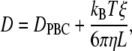
The preceding diffusion constants require two adjustments before they can be usefully compared with experiment. The viscosity, η, of pure TIP3P water at 293 K equals 0.0035 P (31), which is substantially less than the experimental value of 0.01 P (46). Assuming that the underestimation is the same for the polymer solutions at 296 K, where the viscosity of pure water is 0.00933 P, the diffusion constants were scaled by a factor of 0.0035/0.00933 = 0.375. DPBC also requires the following finite size correction developed by Yeh and Hummer (47),
 |
(4) |
where kB is Boltzmann's constant, L is the cubic box length, and ξ = 2.837297. The increase in viscosity effected by the presence of polymer was estimated by the Einstein formula (18)
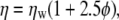 |
(5) |
where ηw is the pure solvent viscosity, and φ is the volume fraction of the particles in the total volume of the suspension; Eq. 5 has been shown to be applicable for low molecular weight PEG (48). Volume fractions for the 9, 18, 27, and 36-mers are 0.0078, 0.0165, 0.0202, and 0.0125, respectively, yielding corrections of 2–5%. The value for the simulated diffusion constant with both corrections,  is
is
 |
(6) |
Hydrodynamic radii of the polymers were then calculated from the Stokes-Einstein relationship for a sphere with stick boundary conditions (43):
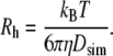 |
(7) |
Calculation of the diffusion coefficient from hydrodynamic bead model
Translational diffusion constants of PEO and PEG were also obtained using the hydrodynamic bead model developed by Garcia de la Torre and Bloomfield (32). In this model, atom centers are considered point sources of friction with hydrodynamic interactions described by a specific shielding tensor, in this case the Oseen tensor (32,43). Inversion of the matrix of interactions and subsequent summing of forces yield a rotational and translational diffusion tensor for the array.
For the present application, friction constants  for carbons and oxygens of the polymers were calculated from
  where a = 0.732 Å is the effective bead radius, and η equaled the viscosity of water at 296 K corrected for polymer concentration (Eq. 5). The preceding value for a is the geometric mean of the C-O and C-C bond distances from the parameter set. It is analogous to the value of 0.77 Å (1/2 of the C-C bond length) found appropriate for alkanes (49,50) when calculating diffusion constants using the Kirkwood-Riseman equation (51). It is necessary to explicitly include bound water to the array of beads when modeling diffusion of proteins (52,53), micelles (54,55), and carbohydrates (56,57) in water, so it is expected that some level of bound water is required for solutions of PEO and PEG. Diffusion tensors were evaluated for configurations with no added water, and with waters bound at
 and
and  generated at 500 ps intervals over the 2–20 ns range for each trajectory. The components of the diffusion tensor were averaged to yield
  and
and  and average diffusion constant
  Because the radius of gyration for the largest polymers indicated relaxation within 2 ns as an upper limit, sets of four consecutive data points were averaged to obtain independent estimates of the translational diffusion constants for computing the standard errors. Translational diffusion constants evaluated using the bead model without and with bound water are denoted
  and
and 
RESULTS AND DISCUSSION
Revision of the CHARMM ether force field: conformers of dimethoxyethane
Raman spectroscopy of DME/water solutions at mole fractions 0.3, 0.6, and 1.0 (25) indicates that the principal conformers are TGT, TGG′, TTT, TGG, and TTG, where T and G respectively denote trans, and gauche in the order of C-O-C-C, O-C-C-O and C-C-O-C; GG′ denotes a pair of gauche of opposite signs. As is evident in Table 1 and Fig. 2, trajectories generated by C35 underestimate the populations of TGT and TGG′ and overestimate TTT and TTG. This suggested that stabilization of the gauche state of the central torsion could improve agreement with experiment. The O-C-C-O dihedral potential energy term was refit against the previously calculated gas-phase ab initio surface (24), yielding the revision
 |
(8) |
TABLE 1.
Molecular volume, dielectric constant, heat of vaporization of dimethoxyethane (DME), and conformer populations at three mole fractions from simulation (averaged over the last 1 ns) and experiment
| Simulation
|
||||
|---|---|---|---|---|
| Property | C35 | C35r | Experiment* | |
| Molecular volume (Å3) | 175.4 ± 0.1 | 174.6 ± 0.1 | 173.6 | |
| Dielectric constant | 7.08 ± 0.04 | 7.81 ± 0.04 | 7.22 | |
| Heat of vaporization (kcal/mol) | 9.18 ± 0.08 | 9.09 ± 0.07 | 8.79 | |
| Conformer population | ||||
| Mole fraction = 1.0 | TGT | 0.341 ± 0.002 | 0.392 ± 0.002 | 0.395 ± 0.030 |
| TGG′ | 0.268 ± 0.003 | 0.283 ± 0.003 | 0.340 ± 0.030 | |
| TTT | 0.195 ± 0.003 | 0.141 ± 0.001 | 0.120 ± 0.020 | |
| TTG | 0.111 ± 0.001 | 0.081 ± 0.001 | 0.050 ± 0.020 | |
| TGG | 0.085 ± 0.001 | 0.103 ± 0.001 | 0.095 ± 0.020 | |
| Mole fraction = 0.6 | TGT | 0.434 ± 0.002 | 0.477 ± 0.003 | 0.480 ± 0.040 |
| TGG′ | 0.220 ± 0.003 | 0.230 ± 0.002 | 0.260 ± 0.030 | |
| TTT | 0.153 ± 0.002 | 0.107 ± 0.001 | 0.090 ± 0.010 | |
| TTG | 0.086 ± 0.001 | 0.063 ± 0.001 | 0.045 ± 0.020 | |
| TGG | 0.107 ± 0.002 | 0.123 ± 0.001 | 0.125 ± 0.030 | |
| Mole fraction = 0.3 | TGT | 0.520 ± 0.005 | 0.564 ± 0.003 | 0.550 ± 0.040 |
| TGG′ | 0.173 ± 0.004 | 0.172 ± 0.003 | 0.205 ± 0.030 | |
| TTT | 0.110 ± 0.001 | 0.074 ± 0.001 | 0.050 ± 0.010 | |
| TTG | 0.067 ± 0.001 | 0.045 ± 0.002 | 0.040 ± 0.020 | |
| TGG | 0.130 ± 0.004 | 0.145 ± 0.001 | 0.155 ± 0.030 | |
FIGURE 2.

Conformer populations for DME for three mole fractions from experiment (squares), and simulations with C35 (triangles) and C35r (solid circles).
All other terms in C35r are the same as those in C35. Fig. 3 plots selected torsional scans to illustrate the difference between the two parameter sets. Table 1 and Fig. 2 show improved agreement with experiment at all three mole fractions for DME conformers generated with C35r. The molecular volume, dielectric constant, and heat of vaporization also agree well with experiment (Table 1).
FIGURE 3.

Potential energies of O-C-C-O with adjacent C-C-O-C in trans (top); O-C-C-O with C-C-O-C gauche and C-C-O-C trans (middle); C-O-C-C with O-C-C-O and C-O-C-C trans (bottom).
Persistence length of polyethylene oxide
To examine the effect of the FF revision on properties of longer chains, simulations were carried out on 9, 18, 27, and 36-mers of PEO in water and 27-mers of PEG using both C35 and C35r. Fig. 4 (top) plots the instantaneous values of the end-to-end distance and the radius of gyration for PEO36. Although fluctuations are clearly higher for h (Table 2), their autocorrelation functions are similar as expected for these closely related quantities (Fig. 4, bottom). The ∼1 ns decay time justifies the 2 ns block size used to calculate statistical errors, and not averaging over the first 2 ns of the 20 ns trajectories to account for equilibration. Values for  and
and  from C35r are slightly lower than those with C35, as expected from the increased population of gauche conformers in the O-C-C-O dihedral angle. Entries in Table 2 for PEO27 and PEG27 are statistically equal for each parameter set, indicating that the differences of the terminal groups do not significantly change their properties.
FIGURE 4.

Time series of the end-to-end distance (h) and radius of gyration ( ) for 36-mers of PEO with C35r (top), and their autocorrelation functions (bottom).
TABLE 2.
Mean-squared end-to-end distance  and radius of gyration
  and their root mean-square fluctuations,
  and
and  (in Å2) of PEO and PEG, averaged over the last 18 ns of each simulation
| Force field | Name ( ) ) |
〈h2〉 |  |
 |
 |
|---|---|---|---|---|---|
| C35 | PEO9 | 258 ± 16 | 151 | 44 ± 1 | 11 |
| (442) | 289 ± 15 | 159 | 46 ± 1 | 12 | |
| PEO18 | 542 ± 45 | 324 | 91 ± 5 | 29 | |
| (838) | 429 ± 47 | 316 | 76 ± 5 | 29 | |
| PEO27 | 973 ± 70 | 515 | 149 ± 10 | 46 | |
| (1234) | 700 ± 114 | 494 | 126 ± 10 | 46 | |
| PEO36 | 1316 ± 145 | 785 | 204 ± 17 | 67 | |
| (1630) | 1230 ± 259 | 898 | 183 ± 26 | 84 | |
| PEG27 | 798 ± 100 | 491 | 133 ± 9 | 46 | |
| (1250) | 910 ± 195 | 658 | 144 ± 21 | 60 | |
| C35r | PEO9 | 229 ± 16 | 147 | 40 ± 1 | 11 |
| (442) | 254 ± 16 | 148 | 43 ± 1 | 11 | |
| PEO18 | 386 ± 40 | 280 | 74 ± 4 | 25 | |
| (838) | 418 ± 55 | 295 | 79 ± 5 | 27 | |
| PEO27 | 765 ± 105 | 523 | 125 ± 9 | 42 | |
| (1234) | 754 ± 147 | 480 | 129 ± 12 | 41 | |
| PEO36 | 1098 ± 295 | 760 | 181 ± 65 | 68 | |
| (1630) | 967 ± 198 | 696 | 169 ± 21 | 70 | |
| PEG27 | 878 ± 156 | 554 | 141 ± 24 | 49 | |
| (1250) | 614 ± 107 | 463 | 115 ± 11 | 46 |
Molecular weights (in daltons) of each polymer are listed in parenthesis below the name.
Fig. 5 plots the molecular weight ( ) dependence of
  for PEO, and linear fits yield the coefficient
  in
in  equal to 0.5 within statistical error. Hence, the PEO behaves as an ideal chain (18). This result is consistent with polymer theory. For high molecular weight polymers in “good solvents” (such as water for PEO), mean field and renormalization group treatments of excluded volume interactions yield
  and 0.588, respectively (58);
  has been experimentally determined for PEO in water for 80,000 <
  (59). However, effects of excluded volume interactions diminish at low
  and
and  (58). Solvent systems can also be developed for real polymers for which
  these are so-called “θ-conditions”.
FIGURE 5.

log  versus log Mw from simulations of PEO.
It is difficult to predict analytically the molecular weight for which nonideality becomes important for a particular polymer, and the following subsection compares hydrodynamic radii obtained from simulation and experiment to demonstrate that  is correct for the present set. For this subsection, the preceding result justifies the use of the worm-like chain model (Eq. 2) to estimate persistence lengths (λ) from simulation, and to compare them to those obtained experimentally for much higher molecular weight PEO. Nonlinear fitting of the simulated
  to Eq. 2 (see Methods) yields λ = 4.3 ± 0.3 Å for C35 and 3.7 ± 0.4 Å for C35r. The slightly larger value for C35 is consistent with the larger values of
  obtained for each molecular weight.
Mark and Flory (28) obtained a characteristic ratio  for high
  PEO in aqueous K2SO4 at 308 K (θ-conditions). Correcting for temperature and applying Eq. 3 yields λ = 3.73 ± 0.29 Å. More recently, Kienberger et al. (29) measured the persistence length of 3.80 ± 0.02 for PEG in saline solution using atomic force microscopy. Both experimental measurements are in quantitative agreement with the value from C35r.
Chain properties obtained here for PEO are similar, though not identical, to those obtained with the parameter set of Bedrov, Borodin, and Smith (BBS) (60,61). Specifically, extrapolating results for the 11-mer reported by them (60) to the temperature of the present simulations yields  Å2; interpolating between results the PEO-9 and PEO-18 yields
  Å2 for C35 and 47 Å2 for C35r. To understand this difference,
  and
and  the probabilities of trans in the central and terminal dihedrals of DME, respectively, were evaluated for the three FF. Interpolating from the mole fractions presented by BBS (61),
  for BBS is between those of C35 and C35r. In contrast, for mole fractions 1, 0.6, and 0.3,
  0.835, and 0.862, respectively, for BBS, whereas
  0.792–0.794, and 0.815–0.819 for C35 and C35r. This increased
  of DME is the likely reason for the higher radius of gyration for PEO in simulations carried out with the BBS force field.
Translational diffusion constant and hydrodynamic radius
Columns 3–5 of Table 3 list  (the translational diffusion constants directly from the trajectories),
  (the correction from Eq. 6), and
  (the hydrodynamic radius calculated from Eq. 7). As expected, the diffusion constants decrease and
  increases with molecular weight, and the statistical error is substantial (as high as 45% for PEO-36). As a check of the validity of these values and for characterizing the anisotropy, diffusion constants were calculated using the hydrodynamic bead model. The last two columns of Table 3 list the diffusion constants based on 40 conformations for each length of PEO and PEG, with (
 ) and without (
 ) bound water. Diffusion constants are very similar for C35 and C35r for each case, indicating that the differences in
  between the two FF mostly arise from statistical error. This is not surprising. The diffusion constant may be calculated analytically for a sphere in a viscous solution, whereas a diffusion constant calculated from a short simulation of the same system would contain a huge statistical error. In this case, the conformational populations of the polymers are reasonably averaged, so bead model calculations using these conformations (37 for each trajectory) yield standard errors of 7% or less for all systems.
TABLE 3.
Diffusion coefficients (10−6 cm2s−1) from simulations, and the hydrodynamic bead model
| MD simulation
|
Hydrodynamic bead model
|
|||||
|---|---|---|---|---|---|---|
| Name |  |
 |
 |
 |
 |
|
| C35 | PEO9 | 5.29 ± 0.97 | 3.44 | 6.6 ± 1.2 | 5.11 ± 0.03 | 3.91 ± 0.04 |
| PEO18 | 4.45 ± 0.97 | 3.09 | 7.2 ± 1.6 | 3.51 ± 0.07 | 2.85 ± 0.09 | |
| PEO27 | 2.33 ± 0.15 | 2.29 | 9.7 ± 0.6 | 2.70 ± 0.10 | 2.24 ± 0.13 | |
| PEO36 | 1.42 ± 0.37 | 1.64 | 13.8 ± 3.6 | 2.36 ± 0.11 | 1.98 ± 0.14 | |
| PEG27 | 3.87 ± 0.66 | 2.86 | 7.7 ± 1.3 | 2.71 ± 0.08 | 2.22 ± 0.11 | |
| C35r | PEO9 | 8.88 ± 1.16 | 4.79 | 4.8 ± 0.6 | 5.16 ± 0.03 | 3.94 ± 0.03 |
| PEO18 | 4.12 ± 0.30 | 2.97 | 7.5 ± 0.5 | 3.49 ± 0.05 | 2.80 ± 0.06 | |
| PEO27 | 2.21 ± 0.32 | 2.24 | 9.9 ± 1.4 | 2.73 ± 0.08 | 2.26 ± 0.10 | |
| PEO36 | 1.64 ± 0.74 | 1.72 | 13.1 ± 5.9 | 2.39 ± 0.12 | 2.01 ± 0.14 | |
| PEG27 | 1.57 ± 0.53 | 2.00 | 11.0 ± 3.7 | 2.71 ± 0.08 | 2.23 ± 0.12 | |
 is obtained directly from the trajectories, and
  is corrected for finite size effects and the low viscosity of the TIP3P water model using Eq. 6. Hydrodynamic radii,
  (in Å), are calculated from
  and Eq. 7. Diffusion constants for the bead model are evaluated without bound water,
  and with hydration at 2
  level (∼1.5 waters per oxygen),
 are, on average, 24% higher than
  Although this could be ascribed to an error in scaling the viscosities, as explained in the Methods a hydration shell must be included when calculating diffusion constants of water-soluble polymers. Coordinate sets were therefore generated with increasing levels of bound water based on the polymer-water interaction energies. Cutoffs 3 kBT (1.1 waters per monomer), 2 kBT (1.5 waters), and kBT (3.2 waters) yielded average differences with
  of 6.5%, 0.8%, and −15%, respectively. Hence, the 2 kBT level provides the best match. This level of hydration is consistent with previous ones for carbohydrates (56,57), where ∼1 bound water per hydroxyl group provided optimal agreement with experimental rotational and translational diffusion measurements. The radial distribution functions plotted in Fig. 6 demonstrate that the bound waters are closely associated with the oxygens of the PEO chain. Consequently, the diffusion constants and hydrodynamic radii obtained from the MD simulations are reasonable, and may be used for further analysis.
FIGURE 6.

Radial PEO-water distribution functions from simulations of the 9-mer (solid) and 36-mer (dashed) based on C35r for all neighboring waters (unrestricted) and only those whose binding energy equaled 2  or greater.
Fig. 7 shows the good agreement of  obtained from simulation and experiment (26). A linear fit of the experimental
  versus
  yields
 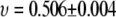 for 200 <
  and
and  for 2000 <
  This further supports the simulation result
  (C35) and 0.515 ± 0.023 (C35r) for 442 <
  (Fig. 5); i.e., PEO at a low molecular weight is appropriately modeled as a worm-like chain in a θ-solvent.
FIGURE 7.

Hydrodynamic radii ( ) of PEO versus molecular weight for C35 (diamonds), C35r (squares); experimental values (26) (triangles) are for PEG.
The relationship of polymer shape and hydrodynamic radius
The excellent agreement of simulation and experiment for λ,  and
and  indicates that the parameter set C35r yields structures that accurately reflect the conformation of PEO and PEG in solution. The top and middle panels of Fig. 8 compare two such structures of PEO-36 (with waters bound at the 2 kBT level) with the hydrodynamic radius evaluated from the average of all structures. The bottom panel shows 20 (from 2 ns intervals) in a common alignment. As anticipated from Eq. 1, the length along the long axis (Z) is substantially larger than the hydrodynamic diameter. However, dimensions along the other two axes are clearly comparable to the hydrodynamic diameter,
  Table 4 lists the averages for all four PEO. The length along X (the middle axis) is ∼1 Å smaller than 2
  for each of the four polymers; the length along Z is comparable to
  Values of the root mean-squared fluctuations are 21%, 17%, and 16% of the lengths along the Z, X, and Y axes, respectively. This result explains the curious relationship between the pore radius
  of membrane proteins and
  Polymers such as PEG in all likelihood diffuse through the pore aligned along their long axes, so the relevant size of the polymer equals
  to within an angstrom.
FIGURE 8.

Side (left) and end-on (right) views of extended (top) and compact (middle) configurations from a trajectory of PEO36 simulated with C35r. PEO carbons and oxygens are blue and red, respectively; waters interacting at the 2  level are green spheres; and the hydrodynamic radius of PEO36 evaluated from hydrodynamics of the chain conformations
  is represented as a transparent sphere positioned in the center of mass. The bottom panel shows the superposition of 20 snapshots at 2 ns intervals, each aligned similarly. The images were created with Visual Molecular Dynamics (67).
TABLE 4.
Average lengths from independent alignments of C35r PEO coordinate sets (including bound water at 2  hydration level) along the three Cartesian axis, assigned in the order Z > X > Y
| Name | Z | X | Y |  |
 |
|---|---|---|---|---|---|
| PEO9 | 18.2 ± 0.1 | 9.9 ± 0.04 | 7.1 ± 0.04 | 15.5 ± 0.7 | 11.6 ± 0.1 |
| PEO18 | 25.3 ± 0.4 | 14.4 ± 0.1 | 10.2 ± 0.1 | 20.0 ± 1.8 | 15.9 ± 0.3 |
| PEO27 | 33.4 ± 0.6 | 18.9 ± 0.2 | 12.6 ± 0.1 | 27.6 ± 3.2 | 19.9 ± 0.9 |
| PEO36 | 39.5 ± 1.1 | 21.8 ± 0.3 | 14.8 ± 0.1 | 32.1 ± 5.4 | 22.4 ± 1.6 |

The ratios Z/X/Y averaged over the PEO listed in Table 4 are 2.59:1.44:1.00. Further averaging X and Y leads to an aspect ratio of 2.13, in agreement with the value of 2.2 obtained experimentally for DNA (23). The results presented here do not speak to the diffusion constant of PEG or PEO while diffusing through a pore (62,63). Interaction with the pore atoms would be expected to modulate the diffusion. Nevertheless, it is useful to note that the bead calculations yield individual elements of the diffusion tensors, and hence the anisotropy. These are  This relatively small diffusional anisotropy is consistent with the shape.
The final topic of this article regards Eq. 1. This equation is derived from the Kirkwood-Riseman (KR) model for polymer diffusion (51), which assumes preaveraging of the Oseen tensor; i.e., the hydrodynamic interactions between beads are evaluated from the average, not instantaneous, distances. This highly useful assumption has been examined by a number of theoretical methods (64–66), leading to the conclusion that the exact diffusion constant is ∼10% lower than that predicted by the KR equation. This implies that the coefficient b in  should be >0.665. The present bead model calculations were carried out on each conformations (i.e., there is no preaveraging) and so provide another test of the KR equation. A comparison of results with and without hydration also speaks to the applicably of Eq. 1. Fig. 9 plots
  (with no bound waters and with hydration at the 2 kBT level) versus
  (for the polymer only);
  was taken from the hydrodynamic calculations to reduce scatter. A linear fit to the function
  yields a slope b = 0.70 and 0.85 for unhydrated and hydrated PEO, respectively. As expected, the former slope is slightly higher than 0.665 in Eq. 1. However, that hydration is the more important effect to consider, and may lead to nonlinearity at higher molecular weights.
FIGURE 9.

Hydrodynamic radius versus radius of gyration from simulations based on C35r. The dashed and solid lines represent linear fits of  obtained from bead model calculations on hydrated and unhydrated PEO, respectively.
CONCLUSIONS
The CHARMM ether force field C35 developed by Vorobyov et al. (24) was revised by adjusting the dihedral potentials to match experimentally measured conformational populations for dimethoxyethane at different mole fractions and the previously published ab initio potential energy surface. MD simulations of 9, 18, 27, and 36-mers of PEO, and 27-mers of PEG based on the revised FF C35r, yield excellent agreement with experiment for persistence lengths and hydrodynamic radii at high and low molecular weights, respectively. In the  regime studied, PEO behaves much like an ideal chain;
  in
in  equals 0.5 within statistical error. The properties of the 27-mers for PEO and PEG are statistically equivalent, and conclusions presented are applicable to both polymers.
The shape anisotropy of hydrated PEO simulated here is 2.59:1.44:1.00. Somewhat remarkably, the middle dimension is only ∼1 Å larger than twice the hydrodynamic radius  This explains the correspondence of
  and
and  the radius of membrane pores: a polymer such as PEG diffuses with its long axis parallel to the membrane channel, so that the effective radius is approximately
  It also implies that the polymer does not substantially distort from its solution shape while diffusing through relatively cylindrical membrane channels. Conversely, a breakdown in the relationship
  is expected to occur for irregularly shaped pores.
Lastly, the present simulations and analyses indicate that  for low molecular PEG and PEO in solution. This increase in the constant of proportionally from 0.665 (18) deduced from the Kirkwood-Riseman equation (51) primarily arises from waters of hydration.
Acknowledgments
We thank Sergey Bezrukov for helpful discussions.
This research was supported in part by the Intramural Research Program of the National Institutes of Health, National Heart, Lung, and Blood Institute, and by National Institutes of Health grants GM51501 and GM070855 to A.D.M. This study utilized the high-performance computational capabilities of the Center for Information Technology Biowulf/LoBoS3 and National Heart, Lung, and Blood Institute LoBoS clusters at the National Institutes of Health, Bethesda, MD.
Editor: Klaus Schulten.
References
- 1.Harris, J. M., and R. B. Chess. 2003. Effect of pegylation on pharmaceuticals. Nat. Rev. Drug Discov. 2:214–221. [DOI] [PubMed] [Google Scholar]
- 2.Viossat, B., F. T. Greenaway, G. Morgant, J. C. Daran, N. H. Dung, and J. R. J. Sorenson. 2005. Low-temperature (180 K) crystal structures of tetrakis-mu-(niflumato)di(aqua)dicopper(II) N,N-dimethylformamide and N,N-dimethylacetamide solvates, their EPR properties, and anticonvulsant activities of these and other ternary binuclear copper(II)niflumate complexes. J. Inorg. Biochem. 99:355–367. [DOI] [PubMed] [Google Scholar]
- 3.Lascombe, M. B., M. L. Milat, J. P. Blein, F. Panabieres, M. Ponchet, and T. Prange. 2000. Crystallization and preliminary X-ray studies of oligandrin, a sterol-carrier elicitor from Pythium oligandrum. Acta Crystallogr. D Biol. Crystallogr. 56:1498–1500. [DOI] [PubMed] [Google Scholar]
- 4.Berejnov, V., N. S. Husseini, O. A. Alsaied, and R. E. Thorne. 2006. Effects of cryoprotectant concentration and cooling rate on vitrification of aqueous solutions. J. Appl. Cryst. 39:244–251. [Google Scholar]
- 5.Acharya, S. A., V. N. Acharya, N. D. Kanika, A. G. Tsai, M. Intaglietta, and B. N. Manjula. 2007. Non-hypertensive tetraPEGylated canine haemoglobin: correlation between PEGylation, O-2 affinity and tissue oxygenation. Biochem. J. 405:503–511. [DOI] [PMC free article] [PubMed] [Google Scholar]
- 6.Braun, A., P. C. Stenger, H. E. Warriner, J. A. Zasadzinski, K. W. Lu, and H. W. Taeusch. 2007. A freeze-fracture transmission electron microscopy and small angle X-ray diffraction study of the effects of albumin, serum, and polymers on clinical lung surfactant microstructure. Biophys. J. 93:123–139. [DOI] [PMC free article] [PubMed] [Google Scholar]
- 7.Hu, T., B. N. Manjula, D. X. Li, M. Brenowitz, and S. A. Acharya. 2007. Influence of intramolecular cross-links on the molecular, structural and functional properties of PEGylated haemoglobin. Biochem. J. 402:143–151. [DOI] [PMC free article] [PubMed] [Google Scholar]
- 8.Zimmerberg, J., and V. A. Parsegian. 1986. Polymer inaccessible volume changes during opening and closing of a voltage-dependent ionic channel. Nature. 323:36–39. [DOI] [PubMed] [Google Scholar]
- 9.Decad, G. M., and H. Nikaido. 1976. Outer membrane of gram-negative bacteria. 12. molecular-sieving function of cell-wall. J. Bacteriol. 128:325–336. [DOI] [PMC free article] [PubMed] [Google Scholar]
- 10.Robertson, J. W. F., C. G. Rodrigues, V. M. Stanford, K. A. Rubinson, O. V. Krasilnikov, and J. J. Kasianowicz. 2007. Single-molecule mass spectrometry in solution using a solitary nanopore. Proc. Natl. Acad. Sci. USA. 104:8207–8211. [DOI] [PMC free article] [PubMed] [Google Scholar]
- 11.Krasilnikov, O. V., R. Z. Sabirov, V. I. Ternovsky, P. G. Merzliak, and J. N. Muratkhodjaev. 1992. A simple method for the determination of the pore radius of ion channels in planar lipid bilayer-membranes. FEMS Microbiol. Immunol. 105:93–100. [DOI] [PubMed] [Google Scholar]
- 12.Merzlyak, P. G., L. N. Yuldasheva, C. G. Rodrigues, C. M. M. Carneiro, O. V. Krasilnikov, and S. M. Bezrukov. 1999. Polymeric nonelectrolytes to probe pore geometry: Application to the α-toxin transmembrane channel. Biophys. J. 77:3023–3033. [DOI] [PMC free article] [PubMed] [Google Scholar]
- 13.Rostovtseva, T. K., E. M. Nestorovich, and S. M. Bezrukov. 2002. Partitioning of differently sized poly(ethylene glycol)s into OmpF porin. Biophys. J. 82:160–169. [DOI] [PMC free article] [PubMed] [Google Scholar]
- 14.Peyronnet, O., B. Nieman, F. Genereux, V. Vachon, R. Laprade, and J. L. Schwartz. 2002. Estimation of the radius of the pores formed by the Bacillus thuringiensis Cry1C δ-endotoxin in planar lipid bilayers. Biochim. Biophys. Acta. 1567:113–122. [DOI] [PubMed] [Google Scholar]
- 15.Arnold, T., M. Poynor, S. Nussberger, A. N. Lupas, and D. Linke. 2007. Gene duplication of the eight-stranded beta-barrel OmpX produces a functional pore: A scenario for the evolution of transmembrane β-barrels. J. Mol. Biol. 366:1174–1184. [DOI] [PubMed] [Google Scholar]
- 16.Ternovsky, V. I., Y. Okada, and R. Z. Sabirov. 2004. Sizing the pore of the volume-sensitive anion channel by differential polymer partitioning. FEBS Lett. 576:433–436. [DOI] [PubMed] [Google Scholar]
- 17.Desai, S. A., and R. L. Rosenberg. 1997. Pore size of the malaria parasite's nutrient channel. Proc. Natl. Acad. Sci. USA. 94:2045–2049. [DOI] [PMC free article] [PubMed] [Google Scholar]
- 18.Tanford, C. 1961. Physical Chemistry of Macromolecules. John Wiley & Sons, New York.
- 19.Solc, K. 1971. Shape of a random-flight chain. J. Chem. Phys. 55:335–344. [Google Scholar]
- 20.Rudnick, J., and G. Gaspari. 1986. The asphericity of random-walks. J. Phys. A Math. Gen. 19:L191–L193. [Google Scholar]
- 21.Rudnick, J., and G. Gaspari. 1987. The shapes of random-walks. Science. 237:384–389. [DOI] [PubMed] [Google Scholar]
- 22.Triantafillou, M., and R. D. Kamien. 1999. Polymer shape anisotropy and the depletion interaction. Phys. Rev. E Stat. 59:5621–5624. [DOI] [PubMed] [Google Scholar]
- 23.Haber, C., S. A. Ruiz, and D. Wirtz. 2000. Shape anisotropy of a single random-walk polymer. Proc. Natl. Acad. Sci. USA. 97:10792–10795. [DOI] [PMC free article] [PubMed] [Google Scholar]
- 24.Vorobyov, I., V. M. Anisimov, S. Green, R. M. Venable, A. Moser, R. W. Pastor, and A. D. MacKerell. 2007. Additive and classical drude polarizable force fields for linear and cyclic ethers. J. Chem. Theory Comput. 3:1120–1133. [DOI] [PubMed] [Google Scholar]
- 25.Goutev, N., K. Ohno, and H. Matsuura. 2000. Raman spectroscopic study on the conformation of 1,2-dimethoxyethane in the liquid phase and in aqueous solutions. J. Phys. Chem. A. 104:9226–9232. [Google Scholar]
- 26.Kuga, S. 1981. Pore-Size distribution analysis of gel substances by size exclusion chromatography. J. Chromatogr. 206:449–461. [Google Scholar]
- 27.Couper, A., and R. F. T. Stepto. 1969. Diffusion of low-molecular weight poly(ethylene oxide) in water. Trans. Faraday Soc. 65:2486–2496. [Google Scholar]
- 28.Mark, J. E., and P. J. Flory. 1965. The configuration of the polyoxyethylene chain. J. Am. Chem. Soc. 87:1415–1423. [Google Scholar]
- 29.Kienberger, F., V. P. Pastushenko, G. Kada, H. J. Gruber, C. Riener, H. Schindler, and P. Hinterdorfer. 2000. Static and dynamical properties of single poly(ethylene glycol) molecules investigated by force spectroscopy. Single. Mol. 2:123–128. [Google Scholar]
- 30.Jorgensen, W. L., J. Chandrasekhar, J. D. Madura, R. W. Impey, and M. L. Klein. 1983. Comparison of simple potential functions for simulating liquid water. J. Chem. Phys. 79:926–935. [Google Scholar]
- 31.Feller, S. E., R. W. Pastor, A. Rojnuckarin, S. Bogusz, and B. R. Brooks. 1996. Effect of electrostatic force truncation on interfacial and transport properties of water. J. Phys. Chem. 100:17011–17020. [Google Scholar]
- 32.Garcia de la Torre, J., and V. A. Bloomfield. 1981. Hydrodynamic properties of complex, rigid, biological macromolecules—theory and applications. Q. Rev. Biophys. 14:81–139. [DOI] [PubMed] [Google Scholar]
- 33.Brooks, B. R., R. E. Bruccoleri, B. D. Olafson, D. J. States, S. Swaminathan, and M. Karplus. 1983. CHARMM—a program for macromolecular energy, minimization, and dynamics calculations. J. Comput. Chem. 4:187–217. [Google Scholar]
- 34.Durell, S. R., B. R. Brooks, and A. Bennaim. 1994. Solvent-induced forces between two hydrophilic groups. J. Phys. Chem. 98:2198–2202. [Google Scholar]
- 35.Lamoureux, G., and B. Roux. 2003. Modeling induced polarization with classical Drude oscillators: Theory and molecular dynamics simulation algorithm. J. Chem. Phys. 119:3025–3039. [Google Scholar]
- 36.Nosé, S., and M. L. Klein. 1983. A study of solid and liquid carbon tetrafluoride using the constant pressure molecular-dynamics technique. J. Chem. Phys. 78:6928–6939. [Google Scholar]
- 37.Hoover, W. G. 1985. Canonical dynamics—equilibrium phase-space distributions. Phys. Rev. A. 31:1695–1697. [DOI] [PubMed] [Google Scholar]
- 38.Andersen, H. C. 1980. Molecular-dynamics simulations at constant pressure and/or temperature. J. Chem. Phys. 72:2384–2393. [Google Scholar]
- 39.Darden, T., D. York, and L. Pedersen. 1993. Particle mesh Ewald—an NLog(N) method for Ewald sums in large systems. J. Chem. Phys. 98:10089–10092. [Google Scholar]
- 40.Allen, M. P., and D. J. Tildesley. 1987. Computer Simulations of Liquids. Clarendon Press, Oxford, UK.
- 41.Ryckaert, J. P., G. Ciccotti, and H. J. C. Berendsen. 1977. Numerical integration of the Cartesian equations of motion of a system with constraints: molecular dynamics of N-alkanes. J. Comput. Phys. 23:327–341. [Google Scholar]
- 42.Press, W. H., B. P. Flannery, S. A. Teukolsky, and W. T. Vetterling. 1987. Numerical Recipes. Cambridge University Press, Cambridge, UK.
- 43.Cantor, R. R., and P. R. Shimmmel. 1980. Biophysical Chemistry. W. H. Freeman and Co., San Francisco.
- 44.Larson, R. G. 1999. The Structure and Rheology of Complex Fluids. Oxford University Press, New York.
- 45.Flory, P. J. 1969. Statistical Mechanics of Chain Molecules. John Wiley & Sons, New York.
- 46.Lide, D. R. 2000. CRC Handbook. CRC Press, Boca Raton, FL.
- 47.Yeh, I. C., and G. Hummer. 2004. System-size dependence of diffusion coefficients and viscosities from molecular dynamics simulations with periodic boundary conditions. J. Phys. Chem. B. 108:15873–15879. [Google Scholar]
- 48.Stojilkovic, K. S., A. M. Berezhkovskii, V. Y. Zitserman, and S. M. Bezrukov. 2003. Conductivity and microviscosity of electrolyte solutions containing polyethylene glycols. J. Chem. Phys. 119:6973–6978. [Google Scholar]
- 49.Paul, E., and R. M. Mazo. 1968. Calculations of diffusion coefficients of N-alkanes. J. Chem. Phys. 48:1405–1407. [Google Scholar]
- 50.Pastor, R. W., and M. Karplus. 1988. Parametrization of the friction constant for stochastic simulations of polymers. J. Phys. Chem. 92:2636–2641. [Google Scholar]
- 51.Kirkwood, J. G., and J. Riseman. 1948. The intrinsic viscosities and diffusion constants of flexible macromolecules in solution. J. Chem. Phys. 16:565–573. [Google Scholar]
- 52.Venable, R. M., and R. W. Pastor. 1988. Frictional models for stochastic simulations of proteins. Biopolymers. 27:1001–1014. [DOI] [PubMed] [Google Scholar]
- 53.Tjandra, N., S. E. Feller, R. W. Pastor, and A. Bax. 1995. Rotational diffusion anisotropy of human ubiquitin from N-15 NMR relaxation. J. Am. Chem. Soc. 117:12562–12566. [Google Scholar]
- 54.Dixon, A. M., R. M. Venable, R. W. Pastor, and T. E. Bull. 2002. Micelle-bound conformation of a hairpin-forming peptide: Combined NMR and molecular dynamics study. Biopolymers. 65:284–298. [DOI] [PubMed] [Google Scholar]
- 55.Bogusz, S., R. M. Venable, and R. W. Pastor. 2001. Molecular dynamics simulations of octyl glucoside micelles: dynamic properties. J. Phys. Chem. B. 105:8312–8321. [Google Scholar]
- 56.Rundlof, T., R. M. Venable, R. W. Pastor, J. Kowalewski, and G. Widmalm. 1999. Distinguishing anisotropy and flexibility of the pentasaccharide LNF-1 in solution by carbon-13 NMR relaxation and hydrodynamic modeling. J. Am. Chem. Soc. 121:11847–11854. [Google Scholar]
- 57.Dixon, A. M., R. Venable, G. Widmalm, T. E. Bull, and R. W. Pastor. 2003. Application of NMR, molecular simulation, and hydrodynamics to conformational analysis of trisaccharides. Biopolymers. 69:448–460. [DOI] [PubMed] [Google Scholar]
- 58.Doi, M., and S. F. Edwards. 1986. The Theory of Polymer Dynamics. Clarendon Press, Oxford.
- 59.Devanand, K., and J. C. Selser. 1991. Asymptotic-behavior and long-range interactions in aqueous-solutions of poly(ethylene oxide). Macromolecules. 24:5943–5947. [Google Scholar]
- 60.Smith, G. D., D. Bedrov, and O. Borodin. 2000. Conformations and chain dimensions of poly(ethylene oxide) in aqueous solution: a molecular dynamics simulation study. J. Am. Chem. Soc. 122:9548–9549. [Google Scholar]
- 61.Bedrov, D., O. Borodin, and G. D. Smith. 1998. Molecular dynamics simulations of 1,2-dimethoxyethane/water solutions. 1. Conformational and structural properties. J. Phys. Chem. B. 102:5683–5690. [Google Scholar]
- 62.Bezrukov, S. M., I. Vodyanoy, R. A. Brutyan, and J. J. Kasianowicz. 1996. Dynamics and free energy of polymers partitioning into a nanoscale pore. Macromolecules. 29:8517–8522. [Google Scholar]
- 63.Kranenburg, M., and B. Smit. 2005. Phase behavior of model lipid bilayers. J. Phys. Chem. B. 109:6553–6563. [DOI] [PubMed] [Google Scholar]
- 64.Wang, S. Q., J. F. Douglas, and K. F. Freed. 1986. Corrections to preaveraging approximation within the Kirkwood-Riseman model for flexible polymers—calculations to 2nd-order in epsilon with both hydrodynamic and excluded volume interactions. J. Chem. Phys. 85:3674–3687. [Google Scholar]
- 65.Zimm, B. H. 1980. Chain molecule hydrodynamics by the Monte-Carlo method and the validity of the Kirkwood-Riseman approximation. Macromolecules. 13:592–602. [Google Scholar]
- 66.Zwanzig, R. 1966. Translational diffusion in polymer solutions. J. Chem. Phys. 45:1858–1859. [Google Scholar]
- 67.Humphrey, W., A. Dalke, and K. Schulten. 1996. VMD: Visual Molecular Dynamics. J. Mol. Graph. 14:33–38. [DOI] [PubMed] [Google Scholar]