Coupling between somatosensory evoked potentials and hemodynamic response in the rat

Abstract

We studied the relationship between somatosensory evoked potentials (SEP) recorded with scalp electroencephalography (EEG) and hemoglobin responses recorded non-invasively with diffuse optical imaging (DOI) during parametrically varied electrical forepaw stimulation in rats. Using these macroscopic techniques we verified that the hemodynamic response is not linearly coupled to the somatosensory evoked potentials, and that a power or threshold law best describes the coupling between SEP and the hemoglobin response, in agreement with the results of most invasive studies. We decompose the SEP response in three components (P1, N1, and P2) to determine which best predicts the hemoglobin response. We found that N1 and P2 predict the hemoglobin response significantly better than P1 and the input stimuli (S). Previous electrophysiology studies reported in the literature show that P1 originates in layer IV directly from thalamocortical afferents, while N1 and P2 originate in layers I and II and reflect the majority of local cortico-cortical interactions. Our results suggest that the evoked hemoglobin response is driven by the cortical synaptic activity and not by direct thalamic input. The N1 and P2 components, and not P1, need to be considered to correctly interpret neurovascular coupling.

Introduction

The ability to observe functional activation of the human brain has been advancing rapidly through the development of several non-invasive techniques, including positron emission tomography (PET), functional magnetic resonance imaging (fMRI), electroencephalography (EEG), magnetoencephalography (MEG), and diffuse optical imaging (DOI). While these techniques are often used to explore the neurophysiology underlying human behavior, the relationship between these signals and neuronal activity is not completely understood. fMRI, PET and DOI signals reflect brain activity indirectly through changes in local oxygen consumption (CMRO₂), cerebral blood flow (CBF), and cerebral blood volume (CBV). These changes are elicited by neuronal activity, which causes an increase in the regional metabolic demand for oxygen and glucose (Fox et al., 1988; Raichle and Mintun, 2006), followed by a vascular response that involves an increase in the regional blood flow to provide more oxygen and glucose to the tissue (Iadecola, 1993; Lauritzen, 2005). EEG and MEG measure fast (peak latency from tens to hundreds of milliseconds) electrical and magnetic signals, which are more directly related to neuronal activation. Multimodal imaging is required to study the relationship between these electrical signals and the hemodynamic response.

In general, the nature of the relationship between the vascular response and the input stimulus is considered linear and time invariant (LTI) (Nangini et al., 2006). If the transformation is LTI, the hemodynamic response can be predicted using the input stimulus. In addition, a temporal overlap of the hemodynamic responses can be resolved using deconvolution, and the resulting deconvolved responses accurately reflect the hemodynamic response (Bandettini and Ungerleider, 2001). Non-linearity of the fMRI blood oxygen level-dependent (BOLD) response has been observed for short duration stimuli (Birn et al., 2001; Liu and Gao, 2000). Stimuli shorter than 3 sec in duration seem to produce responses larger than predicted by the linear model. The non-linearity measured with BOLD fMRI may be due to non-linearity in the electrical measure of the neuronal response (Arthurs et al., 2006; Van Camp et al., 2006), non-linearity in the hemodynamic response, or both (Bandettini and Ungerleider, 2001). By measuring electrical activity and the vascular response simultaneously, one can test the linearity and time invariance of the electrical to vascular transformation and evaluate the coupling between the measured electrical and hemodynamic responses.

Recently, a great deal of effort has been devoted to studying the nature of the neurovascular coupling by combining invasive electrophysiological measurements of multiunit activity (MUA) and local field potentials (LFP) with measurements of hemoglobin concentration changes using intrinsic optical imaging and spectroscopy (OIS) (Devor et al., 2003; Sheth et al., 2003) or with measurements of cerebral blood flow (CBF) changes using laser Doppler flowmetry (LDF) (Hoffmeyer et al., 2007; Jones et al., 2001; Mathiesen et al., 1998; Ngai et al., 1999; Thomsen et al., 2004; Ureshi et al., 2004). Despite technical difficulties, progress has been made in combining microelectrode recordings of MUA and LFP, or evoked potentials measured on the scalp, with BOLD fMRI (Logothetis et al., 2001). These studies have arrived at differing conclusions with respect to the coupling between neuronal activity and the hemodynamic response, with some finding the coupling to be linear (Logothetis et al., 2001; Matsuura and Kanno, 2001) and others finding it to be non-linear (Devor et al., 2003; Hoffmeyer et al., 2007; Jones et al., 2004; Martindale et al., 2005; Norup Nielsen and Lauritzen, 2001; Sheth et al., 2004). Since, depending on the experimental protocol, the non-linear effects can be small and the signal-to-noise ratio (SNR) of the measurements limited, in many cases both linear and non-linear models fit the data adequately, with no statistically significant differences. In addition, because of the different fields of view of the invasive electrical and vascular measurements, the modalities used to investigate the neurovascular coupling can include different neuronal activity both in size and depth, producing inconsistent results (Devor et al., 2005; Ureshi et al., 2005).

By performing simultaneous noninvasive measurements of the neuronal activity with scalp EEG and the vascular response with diffuse optical imaging (DOI), we can measure the electrical and the hemoglobin responses over most of the rat cerebral cortex. Somatosensory evoked potentials (SEP) are signal-averaged field potentials that primarily reflect synaptic activity in cortical neurons (Martin, 1991). SEP recorded with large diameter (4mm) scalp electrodes lacks good spatial resolution but detects the electrical activity over a wide cortical brain volume. During forepaw stimulation the electrodes near the primary somatosensory cortex (SI) resolve the characteristic SEP components, which correspond to SI activation. DOI has been used to measure hemodynamic evoked responses in several cortical areas in both humans and animals (Boas et al., 2004; Durduran et al., 2004; Gibson et al., 2005; Hillman et al., 2007; Hoshi, 2003; Obrig and Villringer, 1997; Villringer and Chance, 1997). Previously, we have shown that in rats we are able to detect evoked hemodynamic responses both spatially and temporally equivalent to fMRI (Culver et al., 2005; Culver et al., 2003; Siegel et al., 2003). As a result, by combining these two techniques we can study the neurovascular relationship by comparing the SI SEP response with the corresponding hemodynamic SI response. The use of an optical method, instead of fMRI, in combination with EEG allows for artifact-free measurements with an excellent signal-to-noise ratio, since there is no interference between DOI and EEG. This allows us to test the linearity and time invariance of the electrical to vascular transformation macroscopically.

In addition, the high SNR allows us to compare different SEP components (P1, N1 and P2), and evaluate their contribution to the hemodynamic response. By limiting the consideration to specific temporal features of the SEP, we believe we can isolate the part of neuronal activity that causes the local excitatory hemodynamic response that we measure with DOI.

The SEP components in rats are similar to those in humans and primates, and based on their timing and polarity they have different cortical representations (Allison et al., 1989a; Allison et al., 1989b; Arezzo et al., 1981; Di and Barth, 1991; Kulics and Cauller, 1986). Evoked potential responses across primary cortices in the rat have a similar structure, consisting first of a large and narrow positive component, P1, followed within 10 ms by a large negative component, N1, and then by two slow components, P2 and N2, tens of ms after N1. Current-source density analysis (CSD) of laminar profiles of cortical field potentials link P1 to the largest and earliest sinks in layers IV and at the border between V and VI. P1 is the primary evoked potential. It has been extensively investigated since the 1940's (Adrian, 1941), mostly because its persistence during deep anesthesia. The origin of P1 from SI-specific thalamocortical inputs is well established (Mitzdorf, 1985). N1 is associated with the slow, long latency sink in layers I/II (Agmon and Connors, 1991; Kulics and Cauller, 1986) and is generated by excitatory cortical events (Cauller and Kulics, 1991). N1 is reduced during deep anesthesia (Arezzo et al., 1981) and slow-wave sleep (Cauller and Kulics, 1988). The inconsistent source-sink patterns and absence of MUA at longer times makes P2's functional significance unclear (Kulics and Cauller, 1986). It has been suggested that P2 represents the response of surrounding fields and arises from activation of cortico-cortical connections originating in the superficial layers of the central column (Kublik et al., 2001; Wrobel et al., 1998). N1 and P2 reflect the majority of cortico-cortical interactions (Szentagothai, 1978). In this work, by parametrically changing the duration, amplitude, and frequency of the stimulation of the rat forepaw, we can produce different effects in the P1, N1, and P2 components of the SEP, and test which component better correlates with the hemoglobin response. This allows us to determine whether the hemodynamic response is driven by the neuronal input or by the cortical neuronal activity.

Materials and Methods

Animal preparation

Noninvasive optical measurements and scalp electrode EEG measurements were performed simultaneously in 21 male Harlan Sprague-Dawley rats (weight 250-400g). The study was approved by the Animal Care Committee.

The animals were anesthetized with a mixture of 1-1.5% Isoflurane in air for the duration of the surgery. Tracheotomy and cannulation of the femoral artery and vein were performed. Mechanical ventilation was adjusted to maintain physiologic parameters within normal ranges. Following surgery, the rats were fixed to a stereotactic frame and the anesthesia was changed to a 50 mg/kg intravenous bolus of α-chloralose followed by continuous intravenous infusion at 40 mg/kg/hr. Stimulation experiments were delayed by at least 1 hour to allow the anesthetic transition. The area of the head under the optical probe was shaved and the optical probe secured in contact with the head and supported by metal posts. The optical probe covered most of the head and the EEG electrodes were inserted around the probe under the animal skin (see Fig. 1a). The body temperature, respiration, mean arterial blood pressure (MABP), electrocardiogram (ECG) and expired CO₂ were monitored and acquired together with the optical and EEG data. We verified that MABP stayed within the normal range (123±11 mmHg average and standard deviation across all animals) during the experiments.

Figure 1.

a: Position of the optical probe and EEG electrodes relative to the head of the animal. In addition, surface electrodes were positioned on the rat's nose (ground), neck (reference) and torso (2 ECG and one ground). b: oxy and deoxy-hemoglobin concentration changes (HbO and HbR, respectively) maps for one rat during 4 s, 3 Hz, above motor threshold (MT) stimulation. c: Corresponding SEP response due to left forepaw stimulation. Gray vertical line = input stimuli (S), T=total SEP signal. The times to peak of the three SEP components across animals in all experiments were: P1 17±2 ms, N1 31±4 ms, and P2 66±8 ms. We didn't detect a clear N2 component, hence it wasn't considered in our analysis. DOI signals are deconvolved and EEG signals are block averaged in each run and across the 12 runs.

Stimulation protocols

In three different groups of animals, we parametrically varied the stimulus train duration (8 conditions, 6 animals), stimulus current (4 conditions, 9 animals), and stimulus train frequency (8 conditions, 6 animals). We used more animals for the amplitude experiment because of the smaller number of conditions with respect to the other two experiments.

The stimuli were applied using hypodermic needles inserted into the left and right forepaws of the animals. The stimuli were delivered in trains of 200-μs pulses with a maximum current less than 2 mA. The motor threshold (MT) was determined by applying 3 Hz continuous stimulation and adjusting the stimulation current until the forepaw movement was visible (1.3±0.3 mA MT range of current used).

The common condition between the experiments was a 4 s stimulus train duration with amplitude just above MT, and 3 Hz frequency within each train. Keeping two of these three parameters constant, the train duration was varied between 1, 2, 3, 4, 5, 6, 7 and 8 s for the duration experiment; the stimulus current, between 0.5 MT, 0.75 MT, MT and 1.25 MT for the amplitude experiment; and the frequency of the train, between 1, 2, 3, 4, 5, 6, 7 and 8 Hz for the frequency experiment.

The stimulation sequences consisted of up to 24 runs of 6 minutes each per paw, each with 25-35 trains of stimuli. Each run included four conditions. The rest periods between the trains were also random in duration with an average inter-stimulus interval (ISI) of 12 s (the ISI ranged from 2 to 20 s). The stimulation sequences were generated using the algorithm described in (Dale, 1999). Each run was repeated on the right and left forepaw in turn, and the runs corresponding to each side were considered as separate measurements in the analysis.

DOI instrument

We used a multi-channel continuous-wave optical imager (CW4 system, TechEn Inc.), which employs 18 laser diodes and 16 avalanche photodiode detectors (Hamamatsu C5460-01). The instrument is described in more detail elsewhere (Franceschini et al., 2003; Strangman et al., 2002). The 18 laser diodes (nine emitting light at 690 nm, and nine at 830 nm) were frequency-encoded by steps of approximately 200 Hz between 4.0 kHz and 7.4 kHz, so their signals could be acquired simultaneously by the 16 parallel detectors. Each detector's output was digitized at ∼40 kHz. The demodulation of the source signals was performed off-line by using an infinite-impulse-response filter, and finally the signals were converted to 10 Hz time series for analysis.

The optical probe consisted of 9 source fibers (each with two lasers at the two different wavelengths) and 16 detector fibers. To deliver and collect light to and from the probe we used 200-μm multimode silica fibers. The sources and detectors were arranged in 3×3 and 4×4 interleaved grids as show in Fig. 1a and as described in (Siegel et al., 2003). The probe covered a flat region of the rat head extending 7.5 mm either side of the midline, and from 4 mm anterior to 11 mm posterior of the bregma. For the data analysis we considered only the 36 source-detector channels with a 3.5 mm separation.

DOI data analysis

The optical raw data were processed off-line using in-house software implemented in the MATLAB environment (Mathworks Inc., Sherborn, MA). First, the optical signals were temporally co-registered with the EEG signal. The optical signals were then low-pass filtered at 0.5 Hz to reduce the effect of the heartbeat on the hemodynamic signals. The temporal changes in the intensity were translated into temporal changes in the concentrations of oxy-hemoglobin (HbO) and deoxy-hemoglobin (HbR) and total hemoglobin concentration (HbT = HbO+HbR) using the modified Beer-Lambert law. No pathlength correction was performed. From concentration data, the hemodynamic responses to each stimulus condition were calculated using an ordinary least-squares (OLS) linear deconvolution (Serences, 2004). The deconvolved hemoglobin responses were averaged over the measured runs to improve the signal-to-noise ratio with respect to single-run responses. Typical DOI activation maps for both oxy- and deoxy-hemoglobin changes are shown for one rat in Fig. 1b.

From the 36 optical channels we identified the source-detector pair with the most statistically significant oxy-hemoglobin activation in the contralateral SI cortex (dark red area in the HbO panels Fig. 1b, p-value always < 0.05) and used the data of this channel to calculate the hemodynamic response. In a previous paper, in which we tomographically reconstructed the hemoglobin volumetric maps (Culver et al., 2003), we verified that the hemodynamic response is co-localized and at a similar depth of the fMRI hemodynamic response, but the spatial extent of activation resolved with DOI in this configuration is 70% larger than the spatial extent of activation resolved with fMRI: full width half maximum (FWHM) of activation ∼2.6 mm for DOI vs. FWHM of 1.4 mm for contrast agent-based fMRI images of cerebral blood volume (Mandeville et al., 1999). We verified that the estimated hemodynamic response from the tomographic image reconstruction had the same relative magnitudes as that estimated from the individual source-detector channel with the maximum and most statistically significant response. This observation makes sense as the volume covered by a source-detector channel (3.5 mm) is larger than the actual volume of activation and we used wavelengths that minimized hemoglobin cross-talk produced by partial volume errors (Strangman et al., 2003). We further verified that neighboring channels that showed significant activation produced similar results. Hence, because of the simpler analysis and the reduced noise achieved by considering nearest neighbor channels only, we performed our analysis using the channel with largest responses and not the ROI determined with image reconstruction.

To calculate the grand average across animals, we normalized the signals for each animal by the maximum response to all conditions.

EEG system

For the EEG measurements we used a 40-channel monopolar digital amplifier system (NuAmps, Neuroscan labs Inc.). We used six Ag/Agcl disk-type electrodes (4 mm in diameter, Warner Instruments, Hamden CT, USA) to record the neuronal activity. These electrodes were inserted under the skin on the rat's head around the optical probe (see Fig. 1a). An 8 mm diameter ground electrode was positioned above the nose of the animal and a 10 mm diameter reference electrode was positioned on the neck of the animal. Two ECG electrodes, 10 mm in diameter, were positioned on the torso of the animal, on the left and right sides, and an additional ground electrode was positioned more posterior in the animal torso. We used paste to keep the ground, reference, and ECG electrodes in position. We verified that the impedance of the electrodes was smaller than 5KΩ. We verified that the cross-talk between the stimulation and recording systems did not affect the features calculated from the EEG signals.

EEG data analysis

The EEG and ECG measurements were carried out at a sampling frequency of 1 kHz. The EEG signal from each electrode referenced to the neck electrode was high-pass filtered at a -3dB cutoff frequency of 3.5 Hz. A notch filter was applied to suppress 60 Hz interference. The ECG signals from the two electrodes were subtracted from one other and converted to a 10 Hz heart rate time-series. This ECG signal was then used to filter the arterial pulsation from the scalp electrodes using a linear regression model. For our analyses, we used the data from the electrode in close proximity to the contralateral SI as detected by DOI. This electrode also had the largest P1, N1 and P2 response with respect to the other electrodes. We generally observed two or three electrodes (two in the contralateral side and the one in the frontal area) having the P1, N1 and P2 response with the correct polarity and latencies. We verified that the results of our analyses were generally consistent regardless of the electrode we used.

From the averaged responses of the data recorded on each side on each animal, we isolated the three SEP components (P1, N1 and P2) (see Fig, 1c) by evaluating the zero crossings of each. This is because while changing stimulus duration did not change SEP zero crossings (see Fig. 2 middle panels), during amplitude and frequency experiments the zero crossing changed between conditions (see Fig. 3 middle panels), or between first and subsequent stimuli in the train (see Fig. 4 middle panels). Hence we evaluated the zero crossings separately for the first and subsequent peaks in the average trains, and for each stimulation condition for each rat. In addition, changing stimulation amplitude or frequency caused some SEP components to increase in area while maintaining a constant peak amplitude. We therefore used the SEP area and not the peak of the response to account for this effect and consider the whole detected electrical activity. Considering the specific time intervals for P1, N1 and P2, we determined the areas under the curve of each SEP component for each stimulus within a train and the sum of the areas of the three components (T). Since in the literature the peak amplitude (max) of the electrical activity is generally used, we also calculated the peak responses for each SEP component for comparison with the SEP area. To obtain the grand averages across animals, we normalized the signals for each animal by the maximum response to all conditions, in the same way as we did for the hemodynamic responses.

Figure 2.

Temporal SEP and hemoglobin response traces to four different train durations in one animal. Train durations, from top to bottom are 1, 3, 5, 7 s, respectively. Left panels are the SEP responses to stimulation train. Middle panels are the overlapped SEP responses for each individual stimulus in the train. The black trace represents the response to the first stimulus in the train. The right panel illustrates the HbO (red) and HbR (blue) responses for the corresponding train. Both SEP and hemoglobin responses shown are averaged over the same number of trains during all stimulation runs.

Figure 3.

Temporal SEP and hemoglobin response traces to four different amplitudes in one animal. Train amplitudes, from top to bottom are 0.5, 0.75, 1, 1.25 MT (motor threshold), respectively. Left panels are the SEP responses to stimulation train. Middle panels are the overlapped SEP responses for each individual stimulus in the train. The black trace represents the response to the first stimulus in the train. The right panel illustrates the HbO (red) and HbR (blue) responses for the corresponding train. Both SEP and hemoglobin responses shown are averaged over the same number of trains during all stimulation runs.

Figure 4.

Temporal SEP and hemoglobin response traces to four different train frequencies in one animal. Train frequencies, from top to bottom are 1, 3, 5 and 7 Hz, respectively. Left panels are the SEP responses to stimulation train. Middle panels are the overlapped SEP responses for each individual stimulus in the train. The black trace represents the response to the first stimulus in the train. The right panel illustrates the HbO (red) and HbR (blue) responses for the corresponding train. Both SEP and hemoglobin responses shown are averaged over the same number of trains during all stimulation runs.

Testing of the linearity/non-linearity of the SEP and hemodynamic responses

To assess the linearity of the hemoglobin response and the SEP features with respect to the stimulus conditions, and the linearity between the hemoglobin response and SEP features, we considered the integrated responses. Since altering stimulus duration changed the duration of the hemodynamic response but not the peak amplitude (see Fig. 2 right panels), we used the integrated hemodynamic response in our analyses, not the peak amplitude, to take into account the total amount of hemoglobin supplied during stimulation (Birn et al., 2001; Ureshi et al., 2005). We determined the integrated responses by calculating the area under the hemoglobin curves (ΣHbO ΣHbR, and ΣHbT). To evaluate the integrated SEP responses we calculated the sums of the areas (or max) within a train (ΣP1, ΣN1, and ΣP2). ΣT was estimated by calculating the sums of the areas (or max) of the three components. For the stimuli input feature we summed the number of stimuli within a train (ΣS) considering each stimulus amplitude as equal to 1 for the duration and frequency experiments, and equal to the stimulus amplitude (normalized by setting MT=1) for the amplitude experiment. In addition to considering ΣSEP, we also used Σ(SEP²) to compare with ΣHb. We calculated the correlation coefficients (R) to compare results.

Prediction of hemodynamic response using the different SEP components

We estimated linear convolution models between the measured hemoglobin time series and the measured SEP feature time series (P1, N1, P2, and T or S using a linear, a quadratic and a cubic transformation (x), and three different activation thresholds (N_thresh set at 10%, 20% and 30% of peak SEP). For the SEP we used either the area or the max of each response in the averaged trains. For all experiments, the temporal length of the impulse response function (h) was set to 12 s, which corresponded to 120 time samples. We estimate a separate impulse response function for HbO (h_HbO) and HbR (h_HbR). This convolution model is also used in Logothetis et al. (Logothetis et al., 2001) and later in (Martindale et al., 2005) and assumes that the neuronal activity and hemoglobin responses are related by

$$\begin{array}{c}\mathrm{HbO}\left(t\right)=h_{\mathrm{HbO}}\otimes N^x\left(t\right)\cdot u\left(N\left(t\right)-N_{\mathrm{thresh}}\right)+n_{\mathrm{HbO}}\left(t\right),\\ \mathrm{HbR}\left(t\right)=h_{\mathrm{HbR}}\otimes N^x\left(t\right)\cdot u\left(N\left(t\right)-N_{\mathrm{thresh}}\right)+n_{\mathrm{HbR}}\left(t\right),\end{array}$$

where N(t) is the time course of neuronal activity represented by the ΣSEP for each stimulus pulse in the pulse train(i.e., P1, N1, P2, T, and S), HbO(t) and HbR(t) are the time courses of the hemoglobin signals, h_HbO and h_HbR are the hemoglobin response functions, u(N) is the Heaviside step function, and n_HbO and n_HbR include background physiology and measurement noise, which we assume to be mean zero Gaussian white noise. The h_HbO and h_HbR are estimated using least squares linear deconvolution and are estimated simultaneously for all stimulus conditions in a given experiment (i.e., duration, amplitude, or frequency). Predicting the variation in HbO and HbR responses to the different stimulus conditions is then possible using the linear, quadratic or cubic transformation, i.e., we use Σ(SEP^x) where x = 1, 2, or 3, for the linear, quadratic, and cubic models, respectively, and for the threshold models we use ΣSEP unless ΣSEP < threshold in which case we use 0.

Details of the statistical comparisons

We calculated the coefficients of determination (R²) between the measured and modeled hemoglobin concentrations. We used Fisher's Z transform to map the bounded R² values into unbounded Z values, which better satisfy the assumption of normality. We then applied a multifactor ANOVA to test the null hypothesis that there were no differences between R² values across the chromophores HbO, HbR, and HbT, and across animals. Significant differences in the R² values were found between different components of the SEP and models (i.e., linear, quadratic, cubic, and thresholds).

Results

Figures 2, 3, and 4 show typical temporal traces for the SEP and hemoglobin responses to four conditions in three animals, for the duration, amplitude, and frequency experiments. The left panels in the figures report the average SEP responses during the different stimulation trains. In the middle panels we overlap all of the SEP responses from within a train to emphasize the differences in amplitude and response shape between the first and subsequent stimuli within the train (the response to the first stimulus is shown in black). The right panels report the hemoglobin response for the given stimulus train.

When increasing train duration (Fig. 2) the SEP amplitude remains almost constant (left panels); the P1 responses are similar in amplitude and duration during the first and the other stimuli in the train (middle panels); N1 and P2 amplitudes are largest for the first stimulus (black curve) and decrease for the other stimuli in the train. The hemoglobin response (right panel) quickly saturates in amplitude: i.e., hemoglobin amplitude for the 3 s train is the same as the amplitude for 5 or 7 s trains, but continues to grow in duration for longer trains.

Both the SEP and the hemoglobin response amplitudes increase with increasing stimulation amplitude (Fig. 3). Below the motor threshold, there are no amplitude differences for the P1, N1 and P2 responses to the first and the other stimuli in the train (middle panels), while there are differences for the N1 and P2 amplitudes for stimulation above the MT. Increasing stimulation amplitude broadens the three SEP components for all stimuli presented after the first stimulus in the train.

When increasing the stimulation frequency (Fig.4), the SEP amplitudes decrease and the hemoglobin response amplitude has a maximum between 2-3 Hz. At low frequencies the three SEP components are the same for the first and the other stimuli in the train. In contrast, at higher frequencies (>2Hz) for all stimuli presented after the first stimulus in the train, the onset of P1 is delayed and the peak broadened, the N1 component is delayed and its amplitude largely reduced especially for the even stimuli, and the amplitude of P2 is strongly reduced. The behavior of P1 at high frequencies closely matches the responses measured with intracellular recording in layer IV of the rat barrel cortex (Higley and Contreras, 2006). The hemoglobin response at higher frequencies decreases in both amplitude and duration.

The trends shown in figures 2, 3, and 4 are consistent with the results in all of the rats measured. The varying behaviors of the three SEP components in the three experiments enables analysis to determine which component covaries best with the hemodynamic response.

The results of the relationship between integrated SEP or hemodynamic responses versus stimulus condition for the three experiments averaged over all of the animals are shown in Fig. 5 (Figure 1osm in the online supplemental material is the same as Fig. 5 but includes error bars calculated as standard errors). Panels a, b and c report the integrated SEP responses; panels d, e and f report the squared SEP responses Σ(SEP²). In the duration experiment (Fig. 5 panels a and d), the integrated SEP and hemoglobin responses are linear with the input stimuli. The correlation coefficients (R) are ≥0.98 for all SEP components and hemoglobin concentrations. In the amplitude experiment (Fig. 5 panel b), the correlation coefficients between S and integrated SEP P1 or Hb are slightly lower than for duration (R 0.97 and 0.98, respectively). More important, while the P1 SEP component tends to saturate for higher stimulation amplitudes, the hemoglobin response begins to rise only at higher stimulation amplitudes and, in our range of amplitudes, does not saturate for higher amplitudes. ΣN1 and ΣP2 in the range of amplitudes used are linear with S. By considering Σ(SEP²) the dependence of N1 and P2 with the input stimuli becomes very similar to the hemoglobin concentration dependence with S. For the frequency experiment, there is a strong non-linearity of both integrated SEP and hemodynamic responses with S. Moreover N1, P2, T and Hb are anticorrelated with input stimuli, while for P1 the correlation coefficient is positive (P 0.82). The integrated hemodynamic response decreases rapidly with frequency; ΣN1 and ΣP2 decrease more slowly, while ΣP1 does not decrease with frequency. Similar to the amplitude experiment, by considering Σ(SEP²) the dependence of N1 and P2 with S becomes very similar to the dependence of the hemoglobin concentrations with S.

Figure 5.

ΣHbO, ΣHbR, ΣHbT (HbT = total hemoglobin concentration = HbO+HbR) (both left and right panels), ΣSEP (left panels) and Σ(SEP²) (right panels) vs. stimulus conditions for the grand average of all rats. Panels a and d duration, panels b and e amplitude, and panels c and f frequency experiments. The correlation coefficients (R) are reported next to the corresponding traces. In the duration and amplitude experiment (panels a and d), the SEP, the squared SEP and the hemoglobin responses are almost linear with the input stimuli. For the frequency experiment (panels c and f), there is a strong non-linearity and anticorrelation between S and either N1, P2 and T SEP components or hemodynamic responses. In fact, both SEP and the hemodynamic responses decrease with increased frequency. In all experiments the squared SEP dependence on the input stimuli is very close to that of the hemodynamic responses

In general, when using the square of the integrated signals, N1, P2 and T have a similar dependence with input stimuli as the hemoglobin responses, while the P1 dependence with S still differs from the Hb dependence with S. From these figures it can also be noted that oxy-, deoxy- and total hemoglobin concentrations have a very similar dependence on input stimuli and in the following figures only HbO is reported for brevity. Using the peak amplitude (max) instead of the area of the SEP components produces similar results for the duration and amplitude experiments (see Fig. 2osm in the online supplemental material). For the frequency experiment N1 and P2 max decrease more slowly with stimulation frequency and when squared do not overlap as well with the hemodynamic response as when considering the area.

Fig. 6 shows scatter plots of the integrated oxy-hemoglobin response vs. the integrated SEP responses (Figure 3osm in the online supplemental material is the same as Fig. 6 but includes error bars calculated as standard errors). As for Fig. 5, panels a, b and c report ΣSEP; panels d, e and f report Σ(SEP²). In the duration experiment (panels a and d), the integrated SEP responses are linear with the integrated hemoglobin responses (R∼0.98). In the amplitude experiment (panels b and e) the correlation coefficient between the integrated SEP and the hemodynamic response improves by using Σ(SEP²). For the frequency experiment (panel c), the integrated SEP responses are not linear with the hemodynamic responses (R∼0.84-0.94 for N1, P2 and T, and R=-0.52 for P1). By squaring the SEP responses, N1, P2 and T become more linear with the hemodynamic response (R∼0.96-0.98, panel f), while P1 remains nonlinear with HbO (R= 0.18). Using the SEP max instead of the area (Fig. 4osm in the online supplemental material) we obtain similar results for the duration and amplitude experiments but worse linearity between N1 or P2 and HbO for the frequency experiment. P1 linearity with the hemoglobin responses improves by using the max, but the correlation coefficients for P1 are still significantly lower than those for N1 and P2.

Figure 6.

Panels a, b and c show the scatter plots of normalized ΣHbO and ΣSEP components for the grand averages of all rats. Panels d, e and f, the r scatter plots of normalized ΣHbO and Σ(SEP²) components. Panels a and d: duration, b and e: amplitude, c and f: frequency experiments. The correlation coefficients (R) are reported next to the corresponding traces. The results for HbR and HbT, not shown, are similar. In the duration experiment (panels a and d), the integrated SEP responses are linear with the integrated hemoglobin responses. In the amplitude and frequency experiments, the integrated P1 SEP responses are not linear with the hemodynamic responses. For both amplitude and frequency experiments, N1, P2 and T are more linear with the hemodynamic responses by considering Σ(SEP²) (panels e and f) than by using ΣSEP.

Figure 7 shows the measured and predicted HbO results for the grand average over all animals for each condition, for the three experiments for the linear (panels a, b and c) and quadratic (panels d, e and f) convolution models using the SEP area. The measured and predicted HbR and HbT responses behave similarly (not shown). Figure 5osm in the online supplemental material reports the h_HbO and h_HbR for the linear convolution model for the three experiments. The coefficients of determination (R²) between the measured and predicted hemoglobin responses are reported in Fig. 8 and the color coded * above some bars indicates statistically significant higher R² than obtained with the component labeled with the same color as the * (P<0.05, multifactor ANOVA). The predictions by the input stimuli (S) are generally worse than those using most SEP features, indicating that the vascular response is more tightly coupled to the neuronal response.

Figure 7.

Grand average of the measured oxy-hemoglobin (HbO=red) response with predicted hemodynamic response using the input stimuli (S=gray), the SEP components P1 (green), N1 (black), P2 (orange), and the total SEP response (T=purple) using linear (panels a, b and c) and quadratic (panels d, e and f) convolution models. Panels a and d duration experiment; panels b and e amplitude experiment; panels c and f frequency experiment. The input stimuli and the P1 component are not able to predict the hemodynamic response in the amplitude and frequency experiments. Instead N1, P2 and T using a quadratic model are able to predict quite well the hemodynamic response in all experiments.

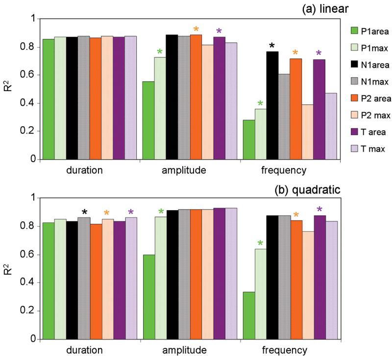
Figure 8.

Coefficients of determination between simulated and measured oxy-hemoglobin response across animals for the linear and quadratic convolution models for the three protocols: duration (a), amplitude (b), and frequency (c). P1 (green), N1 (black), P2 (orange), and the total SEP response (T=purple). Color coded * indicates statistically significant larger R² than for the corresponding color component, P<0.05, multifactor ANOVA. Across the three experiments, the N1 and P2 components consistently provide better R² than P1 and S.

N1 and P2 are able to predict the hemoglobin response quite well across the different experiments, especially with the quadratic convolution model, and generally better than P1. This is best seen during the frequency experiment where the coefficients of determination of the predicted hemodynamic responses have a large magnitude and significant variation from 0.29 for P1 to 0.77-0.71 for N1 and P2 respectively in the linear case, from 0.33 to 0.87-0.84 for the quadratic case. Similarly, with the amplitude experiment P1 R² is significantly smaller than the R² of the other SEP components (0.56 vs. 0.88-0.89 linear, 0.60 vs. 0.91-0.92 quadratic). In the duration experiment because of the strong linearity of hemoglobin concentration with input stimuli we are not able to differentiate between the predictions using different components. In this case, measurement noise reduces the correlations and results in S having a slightly better prediction than the SEP components.

In general we found little difference in predicting the hemodynamic response by using N1, P2 and T. This is because, as previously shown, the amplitude of the P2 component strongly covaries with N1 (Kulics, 1982) and because T strongly covaries with N1 and P2 as ∼87% of its signal is derived from these two components. In fact, averaging across animals, experiments, and conditions, we found N1 contributes 47% and P2 contributes 40%, while P1 contributes only 13% to T.

Figure 9 reports the coefficients of determination using the peak amplitude (max) to predict the hemodynamic response (dashed bars) compared with the results using the area (solid bars). The * above the bars indicates significantly better prediction between area and max for each component. In most cases results are similar. In the duration experiment there is no broadening of the peaks and max and area produce very similar results. In the amplitude and, to a larger extent, in the frequency experiments the broadening of the components plays a role and differences between the analysis using area and max are more evident. In general N1, P2 and T predictions are better using the area, and P1 predictions are better using the max. However, the max P1 does not predict the hemodynamic response as well as the other components. Using the max, the results for P2 predictions are significantly worse than when using the area, probably because P2 is a broad component with a not well-defined peak.

Figure 9.

Comparison of the coefficients of determination between simulated and measured oxy-hemoglobin responses using the SEP area or the SEP peak amplitude (max) as inputs for the linear (panel a) and quadratic (panel b) convolution models. P1 (green), N1 (black), P2 (orange), and the total SEP response (T=purple), solid bars area, dotted bars peak amplitude. For each component * indicates statistically significant larger R² between area and max, P<0.05, multifactor ANOVA. P1 R² is larger using the max than the area in the frequency experiment. Across experiments P2 predictions are significantly worse using the max than using the area.

Using the peak amplitudes the relative contributions to T are 42% for N1, 34% for P1 and 24% for P2. In this case, for the frequency experiment, the prediction using N1 is significantly better than that using T (P value = 0.002) because of the larger weight of P1 on T and the worse ability of P1 and P2 max to predict the hemodynamic response.

Finally, in addition to the linear and quadratic convolution models, for the SEP area we tested a cubic model and a threshold model with the threshold value set at 10, 20 and 30% of the maximum SEP signal (see Fig. 6osm in the online supplemental material). In all cases, the P1 prediction was not as good as N1, P2, and T (p<0.05 for the amplitude and frequency experiments). The linear convolution model works best for all components in the duration experiment (statistically significantly better than quadratic, cubic and threshold 30% models). For the amplitude and frequency experiments, the quadratic and threshold 20% convolution models work best for N1, P2 and T (statistically significantly better than linear, cubic, and threshold 30% models).

Discussion

In vivo and in vitro invasive studies of neurovascular coupling are fundamental for learning the mechanisms of and interplay between neuronal and vascular responses. But it is also important to link these findings with those obtained with the EEG, MEG, MRI, PET, and DOI macroscopic techniques commonly used in humans. In the present study, we used non-invasive macroscopic measures of electrical and vascular activity to investigate the neurovascular coupling in a small animal model. We demonstrate the ability of non-invasive EEG DOI measurements in a small animal model to interrogate the neurovascular coupling, and we are able to bridge between the invasive microscopic studies in animals with the non-invasive macroscopic studies possible in humans. In fact, although EEG and DOI do not provide as high spatial resolution as invasive microscopic techniques, these two modalities offer the advantage of detecting the resultant electrical response from a large population of neurons and the corresponding vascular response from a large number of vessels, as measured non-invasively in humans during standard functional studies. The use of small animals instead of humans allows us to obtain measurements with stronger signal, lower noise, and more repetitions, with a more stable and controlled setup. The results of these non-invasive measurements in rats can be directly translated to human measurements to study neurovascular coupling in humans.

The two major findings of this work are: 1) N1 and P2 SEP components predict the hemodynamic response better than P1; and 2) in agreement with most invasive studies, we determine that the coupling between the electrical and vascular responses is not linear. This non-linearity persists despite the larger field of view of our measurements with respect to LFP and invasive optical imaging measurements, and despite the fact that we used specific components of the SEP signal. We discuss these and other findings in more detail below.

N1 and P2 SEP components predict the hemodynamic response better than P1

In the MUA and LFP electrophysiological studies done to date, the composite electrical signal is compared to the hemodynamic response. In this study, in addition to considering the composite SEP signal, we divided the SEP into three components (P1, N1 and P2) and determined which best correlates with the hemodynamic response. The reason for this analysis is twofold. First, it has been shown that under particular experimental conditions P1 and N1 act differently. When GABA is applied to the cortex, the N1 component is suppressed while the P1 component is preserved (Staba et al., 2004). Similarly, when the cortical surface is cooled, the N1 and P2 components are abolished while P1 remains intact (Kublik et al., 2001). N1 and P2 decrease in amplitude with stimulation frequency and show habituation for high stimulus amplitudes and multiple run repetitions while P1 is less sensitive to changes in stimulation amplitude and frequency (Mitzdorf, 1985; Stienen et al., 2004). This difference in the response between P1 and N1 or P2 allows us to determine that the hemodynamic response matches the N1 and P2 response more closely than the P1 response.

Second, and more important, the fact that these SEP components respond differently to drugs or stimulation paradigms suggest that they represent different populations of neurons. It has been previously shown with topographic studies in the rat cortex that the P1, N1 and P2 temporal components are produced by different subpopulations of pyramidal cells activated both in sequence and in parallel (Di and Barth, 1991; Staba et al., 2003). Current-source density analysis (CSD) of laminar profiles of cortical field potentials link P1 to the largest and earliest sinks in layers IV and at the border between V and VI, and N1 to the slow, long latency sink in layers I/II (Kulics, 1982; Kulics and Cauller, 1986, Agmon, 1991 #4273; Mitzdorf, 1985). Evoked MUA during P1 occurs predominantly at the level of the current sinks, while MUA during N1 appeared at the level of the current sources (Kulics and Cauller, 1986). In fact, although N1 excitation occurs at the border of layers I and II (sink) with excitation of the apical dendrite terminal (Feldman, 1984; Kulics and Cauller, 1986), this excitation leads to discharges in the layer III and V pyramidal cells (sources). MUA reflects mainly the responses of pyramidal cells, which constitute the largest and most numerous cell type in cortical layers III and V (Feldman, 1984; Mountcastle et al., 1969). Inconsistent source-sink patterns and the absence of MUA at later times makes P2's functional significance unclear (Kulics, 1982; Kulics and Cauller, 1986). This component seems to accompany neuronal processing in areas surrounding the central column and derive from a combination of both inhibitory and repolarization processes (Steriade, 1984).

These findings suggest that the cortical hemodynamic response is largely controlled by synaptic activity related to within-cortical processing rather than by direct thalamic input. This is probably because the majority of the synapses within a column input from other neurons in the cortex, and the hemodynamic response is mostly sensitive to the level of synaptic activity (Mathiesen et al., 1998).

We want to emphasize that the measurement techniques we use can detect electrical and hemoglobin activity in layer IV and deeper layers. The fact that the hemodynamic response is best predicted by N1 and P2 SEP components indicates that the vascular response is driven by cortico-cortical synaptic activity originating in superficial layers and not by the layer IV thalamic input activity.

Duration experiment: linearity of the hemodynamic response with SEP

We found linearity between the input stimulus, the vascular response and the electrical responses for the range of durations used. The predictions of the hemoglobin responses using any SEP component or input stimulus are almost identical (R² between 0.86-0.87, Fig. 8 panel a) and the differences are not statistically significant. In the literature, sparser and longer durations have been used to test the linearity of the electrical and vascular responses. Invasive studies in rats using laser Doppler CBF and LFP (Martindale et al., 2005; Ureshi et al., 2004) or SEP from the thinned skull (Ances et al., 2000) have shown non-linearities between the CBF and the neuronal response for durations of 8-16 s. Ureshi et al. (Ureshi et al., 2004) found linearity between integrated CBF and LFP for durations (2, 5, 8, 10 16 s), but intercepts different from zero and a dependence of the slope on frequency of stimulation (0.5, 1, 5 10 Hz); Ances et al. (Ances et al., 2000), using the SEP N1-P2 amplitude, and Martindale et al. (Martindale et al., 2005), with LFP, both found that a non-linear model provided a stronger prediction of CBF than a linear one for stimuli 8 and 16 s long (5 Hz). It has been suggested that the non-linearity at larger stimuli duration is due to the interplay of two different coupling mechanisms for peak and plateau flow responses (Martindale et al., 2005). In our duration experiment we used shorter durations and lower frequency (3Hz) than in the above citations, and we began to see the peak and plateau in the hemoglobin response and small non-linearities between SEP and the hemodynamic response for the 6-8 s duration stimuli (see Fig. 7 panel a). If habituation plays a role in the non-linearity of the electrical response, the use of higher frequency may enhance the effect.

Amplitude experiment: non-linearity of the hemodynamic response with SEP

When changing the stimulus amplitude, we observed small non-linearity between the integrated hemoglobin and N1 and P2 SEP features, and the input stimuli. With amplitude changes, the N1 and P2 SEP components exhibit stronger correlations with the hemoglobin response than P1 and S. The non-linearity we found between P1 (and to a lesser extent N1 and P2) and the hemodynamic response is very similar to the non-linearity between hemodynamic signals and neuronal activity that several groups have noted (Devor et al., 2003; Jones et al., 2004; Norup Nielsen and Lauritzen, 2001; Sheth et al., 2004; Ureshi et al., 2005) using invasive recording of LFP and MUA, LD and OIS in the rat somatosensory cortex. A recent paper compares the total SEP signal with speckle and laser Doppler measurements of blood flow (Royl et al., 2006) by modulating the stimulus amplitude. The non-linear relationship they observed between integrated SEP and CBF is in agreement with our results.

Frequency experiment: non-linearity of the hemodynamic response with SEP

When changing the stimulus frequency, we found the greatest non-linearity of the integrated SEP and hemoglobin responses with the input stimuli. While both the hemodynamic and the SEP responses decrease with increasing frequency, the number of input stimuli increases. The non-linearity of SEP and hemodynamic responses we found is in agreement with results from invasive experiments reported in the literature for which the relationship between the hemodynamic and the integrated LFP responses is non-linear when changing frequency (Hewson-Stoate et al., 2005; Norup Nielsen and Lauritzen, 2001; Sheth et al., 2005). In two papers using SEP measurements, the authors changed stimulation frequencies in the rat forepaw to investigate neurovascular coupling (Ngai et al., 1999; Van Camp et al., 2006). The frequency range and the intervals were greater than in our study (1-12 Hz, 6 conditions in Van Camp et al.; 1-20 Hz, 5 conditions in Ngai et al.). We did not use frequencies higher than 8 Hz and verified that the P2 component ended before 125 ms to avoid overlapping of the SEP responses and interplay of different mechanisms; hence, we cannot perform a direct comparison with these papers. While Van Camp et al. (Van Camp et al., 2006) used the peak-to-peak difference between the P1 and N1 components, Ngai et al. (Ngai et al., 1999) compared the results using the amplitudes of P1 and N1 and found no significant differences between the two. To evaluate the P1 and N1 amplitudes, they used the peak latency times at which the first maximum and minimum occurred, respectively, and used that latency to estimate the P1 and N1 amplitudes for all pulses in the stimulus train. In our data, we observe that while the latency and amplitude of the first P1 and N1 peaks are independent of the stimulation frequency, as expected, the following P1 and N1 peaks in the train are affected in both peak latency (increase) and amplitude (decrease) by increasing frequency. The shift in the peak latency complicates the determination of the peak amplitudes. To minimize this problem we calculated the area under the curves of the SEP components and, to more accurately determine each area, we separately determined the average zero crossings for the first and subsequent peaks in the average stimulus train for each stimulus condition and for each rat.

Comparing non-linear models of the hemodynamic responses

We found that the linear convolution model was able to predict the hemodynamic response in our duration experiment but failed to predict well the hemodynamic response in the amplitude and frequency experiments. We then tested quadratic, cubic, 10%, 20%, and 30% threshold convolution models to determine which better predicts the hemodynamic response. We found that using a quadratic or a 20% threshold convolution model the N1, P2 and T SEP predictions of the hemodynamic response are significantly better across experiments (R²≥ 0.82). Power laws and threshold models have been previously suggested to explain the uncoupling between the electrical and vascular responses (Devor et al., 2003; Norup Nielsen and Lauritzen, 2001; Sheth et al., 2004). The good predictions using a quadratic model can be justified by the fact that the square of the EEG max is a measure of the peak power, and that the square of the EEG response integrated over time is the energy of the local field potential. Hence it is reasonable to think that the energy is driving the hemodynamic response, not the peak power or the field potential. Similarly, as suggested by Norup Nielsen et al. (Norup Nielsen and Lauritzen, 2001), it is possible that a threshold of electrical activity needs to be reached to initiate a vascular response. In our measurements, however, we are unable to determine whether the quadratic or threshold model is more statistically significant.

Area under the curve vs. peak amplitude of SEP components

As input for the models we used either the area under the curve or the amplitude of the peak of each SEP component. While in the literature the peak amplitude of the electrical activity is generally used, we believe the study of the coupling between SEP and the vascular response should be done using the area and not the max. This is because changing the amplitude or frequency of stimulation results in some SEP components becoming larger while maintaining a constant (or decreasing) peak amplitude. By using the SEP area we more accurately account for this effect as confirmed in the analysis of our amplitude and frequency experiments, in which better linearity and better prediction of the hemodynamic response was found using the area versus the max for the N1 and P2 SEP components.

Disagreement between rat and human studies

Human fMRI studies have found non-linearity of the hemodynamic response to short stimuli durations (<2 s)(Birn et al., 2001; Liu and Gao, 2000; Nangini et al., 2006), while animal studies have found non-linearity of the hemodynamic response for long stimuli duration (>8 s) (Ances et al., 2000; Martindale et al., 2005; Ureshi et al., 2004). Martindale et al. (Martindale et al., 2005) suggest that this discrepancy is attributable to different analysis methods. Essentially, the smaller SNR and lower temporal resolution of BOLD fMRI makes problematic the measure at short durations. The impulse response function is generated by the long duration stimuli, which have higher amplitude and better SNR but fail to predict the short stimuli responses, which are then considered non-linear. We have preliminary DOI-MEG results in humans that show similar non-linearity for short durations, as reported in the fMRI literature (data not published). Since with DOI the temporal resolution is not an issue and the SNR for short stimuli duration is adequate, we believe that anesthesia may play a role in the linearity of the short stimuli in rats vs. the non-linearity in non-anesthetized humans.

Measurement field of view

It has been suggested that the non-linearity between electrical and vascular responses measured with invasive techniques when changing stimulation amplitude may be partly caused by the different fields of view of the modalities used (Devor et al., 2005; Ureshi et al., 2005). An increase in stimulation amplitude has been shown to cause an increase in the cortical area of the hemoglobin response (Arthurs et al., 2004; Nemoto et al., 2004). Single electrodes are sensitive to neuronal signals in a small volume of the brain and may not capture all of the neuronal activity associated with the hemodynamic response. In fact, measurements with multiple electrodes (Devor et al., 2005) show that, while the MUA and LFP signals from the electrode in the principal barrel saturate with amplitude, the signals from electrodes in neighboring barrels continue to increase. The hemodynamic response measured in the same experiment with OIS seems to be influenced by the neuronal activity over a broad spatial region. The problem with OIS is that they are typically sensitive only to changes in the most superficial layers of the cortex. This lack of depth resolution may further complicate the interpretation of invasive measurements of the neurovascular coupling. The use of two techniques that measure neuronal and hemodynamic changes over larger volumes is necessary (Hillman et al., 2007).

While we agree that it is critical to understand the differences in spatial sensitivity between the techniques used to measure the hemoglobin response and the neuronal activity, we found that the non-linearity between the electrical and vascular responses persists in our case where the volume-averaged electrical and hemodynamic responses are considered. In fact, when using EEG and DOI, the region of activity is small relative to the spatial sensitivity of the two methods, and included in the measured volume. The hemoglobin response that we measure may change in size with changes in stimulation amplitude due to an increase in the number of vessels that contribute to the hemodynamic signal but is still included in the large detected voxel (∼3.5·2·2 mm³). The corresponding changes in the integrated SEP signal can be due either to an increase in the firing rate or to an increase in the number of firing neurons. Both contributions add up to the measured EEG signal. Thus, by sampling the whole volume of tissue affected by the activity, we overcome the different field of view of the invasive method, but still we found non-linearity between SEP and the hemodynamic response.

Conclusion

In conclusion, we found that the N1 and P2 SEP components allow us to predict the hemoglobin response better than the P1 component or the stimulus input. This is the first experimental confirmation that the hemodynamic response is largely controlled by synaptic activity related to within-cortical processing, rather than by the thalamic input activity. This is probably due to the fact that the majority of the synapses activity derive from cortico-cortical transmission. When the convolution model is used with a quadratic or threshold transformation, the N1 and P2 SEP components, which are representative of these synapses, account for more than 80% of the variance in the hemodynamic responses with our parametrically varying stimuli. We noted that it is important to limit consideration of the neuronal signal to a specific component, as this provides a more specific measure of the neuronal activity responsible for the hemodynamic response. Future effort should consider the possible simultaneous but different contributions from the different SEP components. This effort, however, will require more careful experimental design to provide larger variability in the SEP components to obtain sufficient power in the statistical analyses of the different neurovascular coupling models.

Online supplementary material

01. Figure 1osm.

Same as Fig. 5 but with error bars (standard errors). ΣHbO, ΣHbR, ΣHbT (HbT = total hemoglobin concentration = HbO+HbR) (both left and right panels), ΣSEP (left panels) and Σ(SEP²) (right panels) vs. stimulus conditions for the grand average of all rats. Panels a and d duration, panels b and e amplitude, and panels c and f frequency experiments.

02. Figure 2osm.

Same as Fig. 5 except the max of the SEP components is used instead of the area. ΣHbO, ΣHbR, ΣHbT (HbT = total hemoglobin concentration = HbO+HbR) (both left and right panels), ΣSEP (left panels) and Σ(SEP²) (right panels) vs. stimulus conditions for the grand average of all rats. Panels a and d duration, panels b and e amplitude, and panels c and f frequency experiments. Using the max of the SEP components instead of the area produces similar results for the duration and amplitude experiments. For the frequency experiment, N1 and P2 max decrease more slowly with stimulation frequency, and when squared do not overlap as well with the hemodynamic response as when considering the area.

03. Figure 3osm.

Same as Fig. 6 but with error bars (standard errors). Panels a, b and c show the scatter plots of normalized ΣHbO and ΣSEP components for the grand averages of all rats. Panels d, e and f, the r scatter plots of normalized ΣHbO and Σ(SEP²) components. Panels a and d: duration; b and e: amplitude; c and f: frequency experiments.

04. Figure 4osm.

Same as Fig. 6 but the max of the SEP components is used instead of the area. Panels a, b and c show the scatter plots of normalized ΣHbO and ΣSEP components for the grand averages of all rats. Panels d, e and f, the r scatter plots of normalized ΣHbO and Σ(SEP²) components. Panels a and d: duration; b and e: amplitude; c and f: frequency experiments. Using the SEP max instead of the area, we obtain similar results for the duration and amplitude experiments but slightly worse linearity between N1 or P2 and HbO for the frequency experiment. P1 linearity with the hemoglobin responses improves by using the max, but the correlation coefficients for P1 are still significantly lower than those for N1 and P2.

05. Figure 5osm.

Impulse response functions (h) for HbO (top) and HbR (bottom), obtained by fitting SEP or input stimuli with a linear convolution model. Left panels: duration experiment; middle panels: amplitude experiment; right panels: frequency experiment. For a single stimulus pulse the evoked oxy-hemoglobin concentration takes 2.3-2.5 s to peak, and the deoxy-hemoglobin concentration is slightly delayed (2.5-3 s) with respect to HbO. After 5-5.5 s HbO returns to zero, and after 5.5-6 s HbR returns to zero.

06. Figure 6osm.

Comparison of the coefficients of determination between measured and predicted oxy-hemoglobin responses using different convolution models for P1, N1, P2, and T. We compare linear (dark blue), quadratic (light blue), cubic (green), threshold 10% (t10%=orange), threshold 20% (t20%=red), threshold 30% (t30%=gray) convolution models. For each SEP component, color coded * indicates statistically significant larger R² than for the corresponding convolution model, P<0.05, multifactor ANOVA. In the duration experiment (top panel) the linear convolution model works best for all components. For the amplitude (middle panel) and frequency (bottom panel) experiments, the quadratic and threshold 20% convolution models work best for N1, P2 and T.

References

- Adrian ED. Afferent discharges to the cerebral cortex from peripheral sense organs. J Physiol. 1941;100:159–191. doi: 10.1113/jphysiol.1941.sp003932. [DOI] [PMC free article] [PubMed] [Google Scholar]
- Agmon A, Connors BW. Thalamocortical responses of mouse somatosensory (barrel) cortex in vitro. Neuroscience. 1991;41:365–379. doi: 10.1016/0306-4522(91)90333-j. [DOI] [PubMed] [Google Scholar]
- Allison T, McCarthy G, Wood CC, Darcey TM, Spencer DD, Williamson PD. Human cortical potentials evoked by stimulation of the median nerve. I. Cytoarchitectonic areas generating short-latency activity. J Neurophysiol. 1989a;62:694–710. doi: 10.1152/jn.1989.62.3.694. [DOI] [PubMed] [Google Scholar]
- Allison T, McCarthy G, Wood CC, Williamson PD, Spencer DD. Human cortical potentials evoked by stimulation of the median nerve. II. Cytoarchitectonic areas generating long-latency activity. J Neurophysiol. 1989b;62:711–722. doi: 10.1152/jn.1989.62.3.711. [DOI] [PubMed] [Google Scholar]
- Ances BM, Zarahn E, Greenberg JH, Detre JA. Coupling of neural activation to blood flow in the somatosensory cortex of rats is time-intensity separable, but not linear. J Cereb Blood Flow Metab. 2000;20:921–930. doi: 10.1097/00004647-200006000-00004. [DOI] [PubMed] [Google Scholar]
- Arezzo JC, Vaughan HG, Jr, Legatt AD. Topography and intracranial sources of somatosensory evoked potentials in the monkey. II. Cortical components. Electroencephalogr Clin Neurophysiol. 1981;51:1–18. doi: 10.1016/0013-4694(81)91505-4. [DOI] [PubMed] [Google Scholar]
- Arthurs OJ, Donovan T, Spiegelhalter DJ, Pickard JD, Boniface SJ. Intracortically Distributed Neurovascular Coupling Relationships within and between Human Somatosensory Cortices. Cereb Cortex. 2006 doi: 10.1093/cercor/bhk014. [DOI] [PubMed] [Google Scholar]
- Arthurs OJ, Johansen-Berg H, Matthews PM, Boniface SJ. Attention differentially modulates the coupling of fMRI BOLD and evoked potential signal amplitudes in the human somatosensory cortex. Exp Brain Res. 2004;157:269–274. doi: 10.1007/s00221-003-1827-4. [DOI] [PubMed] [Google Scholar]
- Bandettini PA, Ungerleider LG. From neuron to BOLD: new connections. Nat Neurosci. 2001;4:864–866. doi: 10.1038/nn0901-864. [DOI] [PubMed] [Google Scholar]
- Birn RM, Saad ZS, Bandettini PA. Spatial heterogeneity of the nonlinear dynamics in the FMRI BOLD response. Neuroimage. 2001;14:817–826. doi: 10.1006/nimg.2001.0873. [DOI] [PubMed] [Google Scholar]
- Boas DA, Dale AM, Franceschini MA. Diffuse optical imaging of brain activation: approaches to optimizing image sensitivity, resolution, and accuracy. Neuroimage. 2004;23 1:S275–288. doi: 10.1016/j.neuroimage.2004.07.011. [DOI] [PubMed] [Google Scholar]
- Cauller LJ, Kulics AT. A comparison of awake and sleeping cortical states by analysis of the somatosensory-evoked response of postcentral area 1 in rhesus monkey. Exp Brain Res. 1988;72:584–592. doi: 10.1007/BF00250603. [DOI] [PubMed] [Google Scholar]
- Cauller LJ, Kulics AT. The neural basis of the behaviorally relevant N1 component of the somatosensory-evoked potential in SI cortex of awake monkeys: evidence that backward cortical projections signal conscious touch sensation. Exp Brain Res. 1991;84:607–619. doi: 10.1007/BF00230973. [DOI] [PubMed] [Google Scholar]
- Culver JP, Siegel AM, Franceschini MA, Mandeville JB, Boas DA. Evidence that cerebral blood volume can provide brain activation maps with better spatial resolution than deoxygenated hemoglobin. Neuroimage. 2005;27:947–959. doi: 10.1016/j.neuroimage.2005.05.052. [DOI] [PubMed] [Google Scholar]
- Culver JP, Siegel AM, Stott JJ, Boas DA. Volumetric diffuse optical tomography of brain activity. Opt Lett. 2003;28:2061–2063. doi: 10.1364/ol.28.002061. [DOI] [PubMed] [Google Scholar]
- Dale AM. Optimal experimental design for event-related fMRI. Hum Brain Mapp. 1999;8:109–114. doi: 10.1002/(SICI)1097-0193(1999)8:2/3<109::AID-HBM7>3.0.CO;2-W. [DOI] [PMC free article] [PubMed] [Google Scholar]
- Devor A, Dunn AK, Andermann ML, Ulbert I, Boas DA, Dale AM. Coupling of total hemoglobin concentration, oxygenation, and neural activity in rat somatosensory cortex. Neuron. 2003;39:353–359. doi: 10.1016/s0896-6273(03)00403-3. [DOI] [PubMed] [Google Scholar]
- Devor A, Ulbert I, Dunn AK, Narayanan SN, Jones SR, Andermann ML, Boas DA, Dale AM. Coupling of the cortical hemodynamic response to cortical and thalamic neuronal activity. Proc Natl Acad Sci U S A. 2005;102:3822–3827. doi: 10.1073/pnas.0407789102. [DOI] [PMC free article] [PubMed] [Google Scholar]
- Di S, Barth DS. Topographic analysis of field potentials in rat vibrissa/barrel cortex. Brain Res. 1991;546:106–112. doi: 10.1016/0006-8993(91)91164-v. [DOI] [PubMed] [Google Scholar]
- Durduran T, Burnett MG, Yu G, Zhou C, Furuya D, Yodh AG, Detre JA, Greenberg JH. Spatiotemporal quantification of cerebral blood flow during functional activation in rat somatosensory cortex using laser-speckle flowmetry. J Cereb Blood Flow Metab. 2004;24:518–525. doi: 10.1097/00004647-200405000-00005. [DOI] [PubMed] [Google Scholar]
- Feldman ML. Morphology of the neocortical pyramidal neuron. In: Peters A, Jones EG, editors. Cerebral cortex: cellular components of the corebral cortex. Vol. 1. Plenum Press; New York, London: 1984. pp. 123–200. [Google Scholar]
- Fox PT, Raichle ME, Mintun MA, Dence C. Nonoxidative glucose consumption during focal physiologic neural activity. Science. 1988;241:462–464. doi: 10.1126/science.3260686. [DOI] [PubMed] [Google Scholar]
- Franceschini MA, Fantini S, Thompson JH, Culver JP, Boas DA. Hemodynamic evoked response of the sensorimotor cortex measured noninvasively with near-infrared optical imaging. Psychophysiology. 2003;40:548–560. doi: 10.1111/1469-8986.00057. [DOI] [PMC free article] [PubMed] [Google Scholar]
- Gibson AP, Hebden JC, Arridge SR. Recent advances in diffuse optical imaging. Phys Med Biol. 2005;50:R1–43. doi: 10.1088/0031-9155/50/4/r01. [DOI] [PubMed] [Google Scholar]
- Hewson-Stoate N, Jones M, Martindale J, Berwick J, Mayhew J. Further nonlinearities in neurovascular coupling in rodent barrel cortex. Neuroimage. 2005;24:565–574. doi: 10.1016/j.neuroimage.2004.08.040. [DOI] [PubMed] [Google Scholar]
- Higley MJ, Contreras D. Balanced excitation and inhibition determine spike timing during frequency adaptation. J Neurosci. 2006;26:448–457. doi: 10.1523/JNEUROSCI.3506-05.2006. [DOI] [PMC free article] [PubMed] [Google Scholar]
- Hillman EM, Devor A, Bouchard MB, Dunn AK, Krauss GW, Skoch J, Bacskai BJ, Dale AM, Boas DA. Depth-resolved optical imaging and microscopy of vascular compartment dynamics during somatosensory stimulation. Neuroimage. 2007 doi: 10.1016/j.neuroimage.2006.11.032. [DOI] [PMC free article] [PubMed] [Google Scholar]
- Hoffmeyer HW, Enager P, Thomsen KJ, Lauritzen MJ. Nonlinear neurovascular coupling in rat sensory cortex by activation of transcallosal fibers. J Cereb Blood Flow Metab. 2007;27:575–587. doi: 10.1038/sj.jcbfm.9600372. [DOI] [PubMed] [Google Scholar]
- Hoshi Y. Functional near-infrared optical imaging: utility and limitations in human brain mapping. Psychophysiology. 2003;40:511–520. doi: 10.1111/1469-8986.00053. [DOI] [PubMed] [Google Scholar]
- Iadecola C. Regulation of the cerebral microcirculation during neural activity: is nitric oxide the missing link? Trends Neurosci. 1993;16:206–214. doi: 10.1016/0166-2236(93)90156-g. [DOI] [PubMed] [Google Scholar]
- Jones M, Berwick J, Johnston D, Mayhew J. Concurrent optical imaging spectroscopy and laser-Doppler flowmetry: the relationship between blood flow, oxygenation, and volume in rodent barrel cortex. Neuroimage. 2001;13:1002–1015. doi: 10.1006/nimg.2001.0808. [DOI] [PubMed] [Google Scholar]
- Jones M, Hewson-Stoate N, Martindale J, Redgrave P, Mayhew J. Nonlinear coupling of neural activity and CBF in rodent barrel cortex. Neuroimage. 2004;22:956–965. doi: 10.1016/j.neuroimage.2004.02.007. [DOI] [PubMed] [Google Scholar]
- Kublik E, Musial P, Wrobel A. Identification of principal components in cortical evoked potentials by brief surface cooling. Clin Neurophysiol. 2001;112:1720–1725. doi: 10.1016/s1388-2457(01)00603-4. [DOI] [PubMed] [Google Scholar]
- Kulics AT. Cortical neural evoked correlates of somatosensory stimulus detection in the rhesus monkey. Electroencephalogr Clin Neurophysiol. 1982;53:78–93. doi: 10.1016/0013-4694(82)90108-0. [DOI] [PubMed] [Google Scholar]
- Kulics AT, Cauller LJ. Cerebral cortical somatosensory evoked responses, multiple unit activity and current source-densities: their interrelationships and significance to somatic sensation as revealed by stimulation of the awake monkey's hand. Exp Brain Res. 1986;62:46–60. doi: 10.1007/BF00237402. [DOI] [PubMed] [Google Scholar]
- Lauritzen M. Opinion: Reading vascular changes in brainimaging: is dendritic calcium the key? Nature Reviews Neuroscience. 2005;6:77. doi: 10.1038/nrn1589. [DOI] [PubMed] [Google Scholar]
- Liu H, Gao J. An investigation of the impulse functions for the nonlinear BOLD response in functional MRI. Magn Reson Imaging. 2000;18:931–938. doi: 10.1016/s0730-725x(00)00214-9. [DOI] [PubMed] [Google Scholar]
- Logothetis NK, Pauls J, Augath M, Trinath T, Oeltermann A. Neurophysiological investigation of the basis of the fMRI signal. Nature. 2001;412:150–157. doi: 10.1038/35084005. [DOI] [PubMed] [Google Scholar]
- Mandeville JB, Marota JJA, Ayata C, Moskowitz MA, Weisskoff RM, Rosen BR. An MRI Measurement of the Temporal Evolution of Relative CMRO2 During Rat Forepaw Stimulation. Magn Reson Med In Review. 1999 doi: 10.1002/(sici)1522-2594(199911)42:5<944::aid-mrm15>3.0.co;2-w. [DOI] [PubMed] [Google Scholar]
- Martin JH. The collective electrical behavior of cortical neurons: The Electroencephalogram and the Mechanisms of Epilepsy. In: Kandel ER, Schwartz JH, Jessell TM, editors. Principles of Neural Science. Elsevier; New York: 1991. pp. 771–791. [Google Scholar]
- Martindale J, Berwick J, Martin C, Kong Y, Zheng Y, Mayhew J. Long duration stimuli and nonlinearities in the neural-haemodynamic coupling. J Cereb Blood Flow Metab. 2005;25:651–661. doi: 10.1038/sj.jcbfm.9600060. [DOI] [PubMed] [Google Scholar]
- Mathiesen C, Caesar K, Akgoren N, Lauritzen M. Modification of activity-dependent increases of cerebral blood flow by excitatory synaptic activity and spikes in rat cerebellar cortex. J Physiol. 1998;512(Pt 2):555–566. doi: 10.1111/j.1469-7793.1998.555be.x. [DOI] [PMC free article] [PubMed] [Google Scholar]
- Matsuura T, Kanno I. Quantitative and temporal relationship between local cerebral blood flow and neuronal activation induced by somatosensory stimulation in rats. Neurosci Res. 2001;40:281–290. doi: 10.1016/s0168-0102(01)00236-x. [DOI] [PubMed] [Google Scholar]
- Mitzdorf U. Current source-density method and application in cat cerebral cortex: investigation of evoked potentials and EEG phenomena. Physiol Rev. 1985;65:37–100. doi: 10.1152/physrev.1985.65.1.37. [DOI] [PubMed] [Google Scholar]
- Mountcastle VB, Talbot WH, Sakata H, Hyvarinen J. Cortical neuronal mechanisms in flutter-vibration studied in unanesthetized monkeys. Neuronal periodicity and frequency discrimination. J Neurophysiol. 1969;32:452–484. doi: 10.1152/jn.1969.32.3.452. [DOI] [PubMed] [Google Scholar]
- Nangini C, Ross B, Tam F, Graham SJ. Magnetoencephalographic study of vibrotactile evoked transient and steady-state responses in human somatosensory cortex. Neuroimage. 2006;33:252–262. doi: 10.1016/j.neuroimage.2006.05.045. [DOI] [PubMed] [Google Scholar]
- Nemoto M, Sheth S, Guiou M, Pouratian N, Chen JW, Toga AW. Functional signal- and paradigm-dependent linear relationships between synaptic activity and hemodynamic responses in rat somatosensory cortex. J Neurosci. 2004;24:3850–3861. doi: 10.1523/JNEUROSCI.4870-03.2004. [DOI] [PMC free article] [PubMed] [Google Scholar]
- Ngai AC, Jolley MA, D'Ambrosio R, Meno JR, Winn HR. Frequency-dependent changes in cerebral blood flow and evoked potentials during somatosensory stimulation in the rat. Brain Res. 1999;837:221–228. doi: 10.1016/s0006-8993(99)01649-2. [DOI] [PubMed] [Google Scholar]
- Norup Nielsen A, Lauritzen M. Coupling and uncoupling of activity-dependent increases of neuronal activity and blood flow in rat somatosensory cortex. J Physiol. 2001;533:773–785. doi: 10.1111/j.1469-7793.2001.00773.x. [DOI] [PMC free article] [PubMed] [Google Scholar]
- Obrig H, Villringer A. Near-infrared spectroscopy in functional activation studies. Can NIRS demonstrate cortical activation? Adv Exp Med Biol. 1997;413:113–127. doi: 10.1007/978-1-4899-0056-2_13. [DOI] [PubMed] [Google Scholar]
- Raichle ME, Mintun MA. Brain work and brain imaging. Annu Rev Neurosci. 2006;29:449–476. doi: 10.1146/annurev.neuro.29.051605.112819. [DOI] [PubMed] [Google Scholar]
- Royl G, Leithner C, Sellien H, Muller JP, Megow D, Offenhauser N, Steinbrink J, Kohl-Bareis M, Dirnagl U, Lindauer U. Functional imaging with Laser Speckle Contrast Analysis: Vascular compartment analysis and correlation with Laser Doppler Flowmetry and somatosensory evoked potentials. Brain Research. 2006;1121:95. doi: 10.1016/j.brainres.2006.08.125. [DOI] [PubMed] [Google Scholar]
- Serences JT. A comparison of methods for characterizing the event-related BOLD timeseries in rapid fMRI. Neuroimage. 2004;21:1690–1700. doi: 10.1016/j.neuroimage.2003.12.021. [DOI] [PubMed] [Google Scholar]
- Sheth S, Nemoto M, Guiou M, Walker M, Pouratian N, Toga AW. Evaluation of coupling between optical intrinsic signals and neuronal activity in rat somatosensory cortex. Neuroimage. 2003;19:884–894. doi: 10.1016/s1053-8119(03)00086-7. [DOI] [PubMed] [Google Scholar]
- Sheth SA, Nemoto M, Guiou M, Walker M, Pouratian N, Toga AW. Linear and nonlinear relationships between neuronal activity, oxygen metabolism, and hemodynamic responses. Neuron. 2004;42:347–355. doi: 10.1016/s0896-6273(04)00221-1. [DOI] [PubMed] [Google Scholar]
- Sheth SA, Nemoto M, Guiou MW, Walker MA, Toga AW. Spatiotemporal evolution of functional hemodynamic changes and their relationship to neuronal activity. J Cereb Blood Flow Metab. 2005;25:830–841. doi: 10.1038/sj.jcbfm.9600091. [DOI] [PubMed] [Google Scholar]
- Siegel AM, Culver JP, Mandeville JB, Boas DA. Temporal comparison of functional brain imaging with diffuse optical tomography and fMRI during rat forepaw stimulation. Phys Med Biol. 2003;48:1391–1403. doi: 10.1088/0031-9155/48/10/311. [DOI] [PubMed] [Google Scholar]
- Staba RJ, Bergmann PC, Barth DS. Dissociation of slow waves and fast oscillations above 200 Hz during GABA application in rat somatosensory cortex. J Physiol. 2004;561:205–214. doi: 10.1113/jphysiol.2004.075325. [DOI] [PMC free article] [PubMed] [Google Scholar]
- Staba RJ, Brett-Green B, Paulsen M, Barth DS. Effects of ventrobasal lesion and cortical cooling on fast oscillations (>200 Hz) in rat somatosensory cortex. J Neurophysiol. 2003;89:2380–2388. doi: 10.1152/jn.01098.2002. [DOI] [PubMed] [Google Scholar]
- Steriade M. The excitatory-inhibitory response sequence in thalamic and neocortical cells: staterelated changes and regulatory systems. In: Edelman GM, G W, Cohen WM, editors. Dynamic Aspects of Neocortical Function. John Wiley & Sons; New York: 1984. pp. 107–158. [Google Scholar]
- Stienen PJ, van den Brom WE, de Groot HN, Venker-van Haagen AJ, Hellebrekers LJ. Differences between primary somatosensory cortex- and vertex-derived somatosensory-evoked potentials in the rat. Brain Res. 2004;1030:256–266. doi: 10.1016/j.brainres.2004.10.014. [DOI] [PubMed] [Google Scholar]
- Strangman G, Culver JP, Thompson JH, Boas DA. A quantitative comparison of simultaneous BOLD fMRI and NIRS recordings during functional brain activation. Neuroimage. 2002;17:719–731. [PubMed] [Google Scholar]
- Strangman G, Franceschini MA, Boas DA. Factors affecting the accuracy of near-infrared spectroscopy concentration calculations for focal changes in oxygenation parameters. Neuroimage. 2003;18:865–879. doi: 10.1016/s1053-8119(03)00021-1. [DOI] [PubMed] [Google Scholar]
- Szentagothai J. The Ferrier Lecture, 1977. The neuron network of the cerebral cortex: a functional interpretation. Proc R Soc Lond B Biol Sci. 1978;201:219–248. doi: 10.1098/rspb.1978.0043. [DOI] [PubMed] [Google Scholar]
- Thomsen K, Offenhauser N, Lauritzen M. Principal neuron spiking: neither necessary nor sufficient for cerebral blood flow in rat cerebellum. J Physiol. 2004;560:181–189. doi: 10.1113/jphysiol.2004.068072. [DOI] [PMC free article] [PubMed] [Google Scholar]
- Ureshi M, Kershaw J, Kanno I. Nonlinear correlation between field potential and local cerebral blood flow in rat somatosensory cortex evoked by changing the stimulus current. Neurosci Res. 2005;51:139–145. doi: 10.1016/j.neures.2004.10.008. [DOI] [PubMed] [Google Scholar]
- Ureshi M, Matsuura T, Kanno I. Stimulus frequency dependence of the linear relationship between local cerebral blood flow and field potential evoked by activation of rat somatosensory cortex. Neurosci Res. 2004;48:147–153. doi: 10.1016/j.neures.2003.10.014. [DOI] [PubMed] [Google Scholar]
- Van Camp N, Verhoye M, Van der Linden A. Stimulation of the rat somatosensory cortex at different frequencies and pulse widths. NMR Biomed. 2006;19:10–17. doi: 10.1002/nbm.986. [DOI] [PubMed] [Google Scholar]
- Villringer A, Chance B. Non-invasive optical spectroscopy and imaging of human brain function. Trends Neurosci. 1997;20:435–442. doi: 10.1016/s0166-2236(97)01132-6. [DOI] [PubMed] [Google Scholar]
- Wrobel A, Kublik E, Musial P. Gating of the sensory activity within barrel cortex of the awake rat. Exp Brain Res. 1998;123:117–123. doi: 10.1007/s002210050552. [DOI] [PubMed] [Google Scholar]
Associated Data
This section collects any data citations, data availability statements, or supplementary materials included in this article.
Supplementary Materials