

Abstract
Auditory objects are detected if they differ acoustically from the ongoing background. In simple cases, the appearance or disappearance of an object involves a transition in power, or frequency content, of the ongoing sound. However, it is more realistic that the background and object possess substantial non-stationary statistics, and the task is then to detect a transition in the pattern of ongoing statistics. How does the system detect and process such transitions? We use magnetoencephalography (MEG) to measure early auditory cortical responses to transitions between constant tones, regularly alternating, and randomly alternating tone-pip sequences. Such transitions embody key characteristics of natural auditory temporal edges. Our data demonstrate that the temporal dynamics and response polarity of the neural temporal-edge-detection processes depend in specific ways on the generalized nature of the edge (the context preceding and following the transition) and suggest that distinct neural substrates in core and non-core auditory cortex are recruited depending on the kind of computation (discovery of a violation of regularity, vs. the detection of a new regularity) required to extract the edge from the ongoing fluctuating input entering a listener’s ears.
Section: Cognitive and Behavioral Neuroscience
Keywords: auditory regularity, change detection, M100, M50, Magnetoencephalography, MEG, MMN, scene analysis
Sensitivity to change is a fundamental aspect of hearing: Change detection plays an important role in auditory scene analysis, and also in the perception of complex sound sequences such as speech and music. The brain mechanisms subserving these processes are often studied with the mismatch negativity (MMN) paradigm (Näätänen et al., 1978; Kujala and Näätänen, 2003; Polich, 2003; Winkler, 2008), based on presenting infrequent ‘deviant’ events in a stream of repeating standard events. The MMN component is elicited by sounds violating some regular aspect of the preceding sound sequence (including abstract rules regarding the succession of elements in the sequence; e.g. Wolff and Schröger, 2001; Horvath and Winkler, 2004), and is hypothesized to reflect a discrepancy between the memory trace, or expectations generated by the standard stimulus, and the new, deviant, information (Näätänen, 1992; Sams et al., 1993) or processes that update the internal representation when a previously registered regularity is violated (Winkler et al., 1996; Winkler, 2003). In recent literature, which is dominated by the MMN as an electrophysiological correlate of auditory cortical change detection in humans, ‘change detection’ seems to be equated with ‘violation of regularity’ (e.g. Polich, 2003; Näätänen and Winkler, 1999; Picton et al., 2000; Näätänen et al., 2005; Denham and Winkler, 2006; Schönwiesner et al., 2007; Grimm et al., 2006). However, the opposite side of the coin – the processes by which auditory cortex detects the emergence of regularity out of ‘disorder’ is also a change detection task but has been much less explored (e.g. Haenschel et al., 2005).
An issue closely related to auditory change detection is the detection of ‘temporal edges’ (Fishbach et al., 2001; Herdener et al., 2007): Auditory environments are constantly fluctuating. These fluctuations are due in part to the oscillatory nature of many acoustic sources and in part to the dynamics of their appearance and disappearance from the auditory scene. Presumably, one of the first stages of detecting these onset and offset events, that are superimposed on the already changing input entering a listener’s ears, is the extraction of auditory temporal edges. Whereas ‘edge detection’ has received an enormous amount of attention in the visual literature (e.g. Hubel & Wiesel, 1965; Marr and Hildreth, 1980; Burr et al., 1989; Lamme et al., 1999), the concept is not as extensively explored in the auditory modality. Conceptually, the process of deriving a temporal edge depends on the statistical properties of the stimulus before and after the transition (see e.g. Julesz, 1962 for a discussion of these issues in the visual modality). In some cases, edges are detected as a violation of a previously acquired representation of the scene (this is, as discussed above, the kind of processing tapped by the MMN paradigm), for example when an ongoing auditory object, against some background, disappears or changes it’s properties. In other cases temporal edges are manifested as a transition between random fluctuation and some regular pattern, such as when an auditory source appears out of an ongoing random background. In this situation the change the system has to be able to detect is the emergence of a regularity, or order, out of disorder.
We have recently been exploring these processes of auditory temporal edge detection (Chait et al., 2005; Chait et al., 2007a; Chait et al., 2007b). In a series of MEG experiments we used several different stimulus configurations (dichotic vs. diotic, noiselike vs. tonal, stationary vs. dynamic), that shared the abstract characteristic that they involved a transition from a state of order to disorder, or vice-versa. In one experiment (Chait et al., 2005; see also Chait et al., 2007b) we studied changes in the interaural correlation (IAC) of wide-band noise. Stimuli consisted of interaurally correlated noise (identical noise signals played to the two ears) that changed into uncorrelated noise (different noise signals at the two ears) or vice versa. The stimuli of the second experiment were designed to mimic the abstract properties of those in the IAC experiment, while changing the acoustic properties completely. Signals consisted of a constant tone that changed into a sequence of random tone pips, or vice versa (Chait et al., 2007a). We showed that the temporal dynamics and response morphology of the cortical temporal-edge-detection processes depend in precise ways on the abstract nature of the change. The properties of early auditory cortical responses (from ~50 ms post-transition) to order-disorder edges, and vice versa, demonstrated that some transitions not only require more temporal integration than others, but that this additional integration recruits distinct neural substrates. That similar patterns are observed for stimuli that are dramatically different in every physical sense but that share the same abstract edge properties, suggests the existence of a general edge detection computation that operates early in the processing stream on the abstract statistics of the auditory input.
The present experiment expands the generality of previous findings by investigating more complex auditory temporal edges: We use an ongoing pure tone stimulus with a frequency that is either constant (CONST; a single value for the entire duration of the stimulus), alternating regularly (REG; a regularly alternating sequence of three tone pips) or randomly varying (RAND; a random sequence of tone pips), as well as stimuli that transition from one state to the other (CONST-REG; REG-CONST, RAND-REG, REG-RAND; Figure. 1, see Methods).
Figure 1.
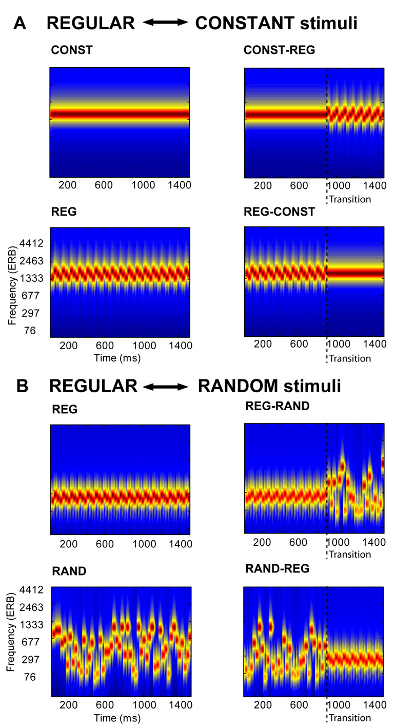
Examples of the stimulus configurations used in the experiment. The plots represent auditory spectrograms, generated with a filterbank of 1/ERB wide channels (Equivalent Rectangular Bandwidth; Moore & Glasberg, 1983) equally spaced on a scale of ERB-rate. Channels are smoothed to obtain a temporal resolution similar to the Equivalent Rectangular Duration (Plack & Moore, 1990). A: In one block, signals were either a constant tone (CONST), a regularly alternating sequence of three tone pips (REG) or contained a transition from constant to regular (CONST-REG) or vice versa (REG-CONST). The blue dashed line marks the transition. An ideal observer is able to detect the CONST-REG transition immediately; however the REG-CONST stimuli are only distinguishable from the REG (control) condition after one pip-duration has elapsed. B: In the other block, signals were either a regularly alternating sequence of three tone-pips (REG), a random sequence of tone-pips of different frequencies (RAND) or contained a transition from regular to random (REG-RAND) or vice versa (RAND-REG). The blue dashed line marks the transition. An ideal observer is able to detect the REG-RAND transition immediately, however the opposite transition (RAND-REG) necessarily takes longer to detect because a listener must wait long enough to distinguish the onset of regularity from an oscillation that might occur by chance.
Theoretically, an ideal observer can immediately detect the transition in the CONST-REG and REG-RAND cases. The first waveform sample that violates the acquired regularity suffices to signal the transition. The opposite transitions—REG-CONST and RAND-REG—necessarily take longer to detect. In the REG-CONST case, the observer must wait an extra pip-duration in order to recognize that a transition has occurred. Similarly, to detect the RAND-REG edge, a listener must wait long enough to distinguish the onset of regularity from an oscillation that might occur by chance.
Importantly, we introduce here a stimulus configuration (RAND-REG) that is distinct from the canonical MMN-eliciting ‘deviation from an established regularity’ design: Whereas REG-CONST, CONST-REG and REG-RAND transitions are characterized by a violation of a preceding regularity (a change in frequency in the case of CONST-REG and REG-RAND, and a mismatch in segment length in the case of REG-CONS) the RAND-REG transition does not violate any regularity and is instead characterized by the emergence of regularity out of disorder.
In our paradigm, listeners were presented with the signals schematized in Figure 1 while performing a decoy task unrelated to change processing. By analyzing the responses to the transitions in the tonal stimuli interspersed between the decoy targets, we identify the neural mechanisms and investigate the computations underlying the detection of the different types of auditory edges.
Results
Constant↔Regular edges
Magnetic waveform and field distribution analyses reveal that participants had comparable response trajectories. Figure 2 shows the root mean square (RMS) of the grand-averaged auditory evoked responses to constant-to-regular (CONST-REG; in grey) and regular-to-constant (REG-CONST; in black) edges. The origin of the time scale coincides with the onset of the signals and the transition occurs at 900 ms post stimulus onset. The evoked MEG activity exhibits a series of deflections at about 100 ms after stimulus onset and a later series of deflections after the transition that begin at about 960 ms post onset (60 ms post transition). These two aspects of the response are discussed, in turn, below.
Figure 2.
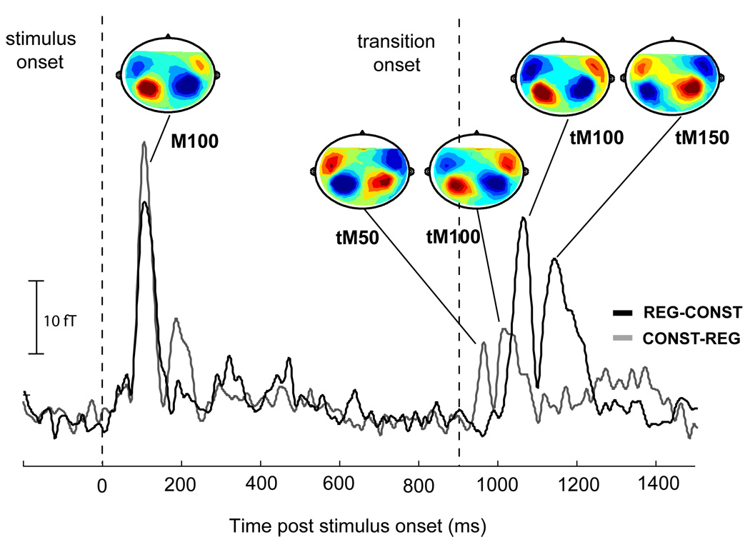
Measured data in the Constant↔Regular block: Root mean square (RMS) of the grand-average (average over all subjects for each of the 156 channels) of the evoked auditory cortical responses to CONST-REG (in grey) and REG-CONST (in black) stimuli. Contour maps at the critical time periods are also provided; Source = red, Sink = blue. Apart from an amplitude difference, onset response dynamics to CONST-REG and REG-CONST stimuli were comparable. Both are characterized by a pronounced M100 onset response at approximately 110 ms post onset, with similar magnetic field distributions. In contrast to the onset responses, transition responses exhibit temporal/morphological differences between conditions. The transition from a constant tone to a regular sequence of tone pips evokes a first deflection (tM50) peaking at about 70 ms post transition, with an M50-like magnetic field polarity, followed by a deflection at about 120 ms post transition (tM100), with an M100-like magnetic field polarity. The first response to REG-CONST transition (tM100) peaks at about 160 ms post transition, with an M100-like magnetic field pattern, followed by a deflection at about 250 ms post transition (tM150) with an M150 dipolar distribution. All statistical analyses were performed on each-hemisphere, subject-by-subject (based on the 10 channels selected for each in each hemisphere). The grand-average plot is shown here for illustration purposes only.
Onset Response
Onset responses to both conditions had similar dynamics (latency and shape of the deflection) and magnetic field distributions. Specifically, both conditions produced a prominent onset response with a peak at approximately 110 ms post onset with a characteristic M100 field distribution (see Fig 2). A repeated measures ANOVA on peak latencies revealed no significant differences. A repeated measures ANOVA on peak amplitudes, with hemisphere and condition as factors revealed a main effect of condition (F(1,11)=11.2, p=0.007) –stemming from the fact that responses to CONST onsets exhibited higher amplitudes than those to REG onsets (see also Chait et al., 2007a). There also appears to be a difference between conditions at around 200 ms post onset – with CONST exhibiting a deflection that is lacking in REG. However, this response is inconsistent across subjects and stimulus repetitions (REG conditions in other blocks do seem to exhibit such a deflection; see Fig 4).
Figure 4.
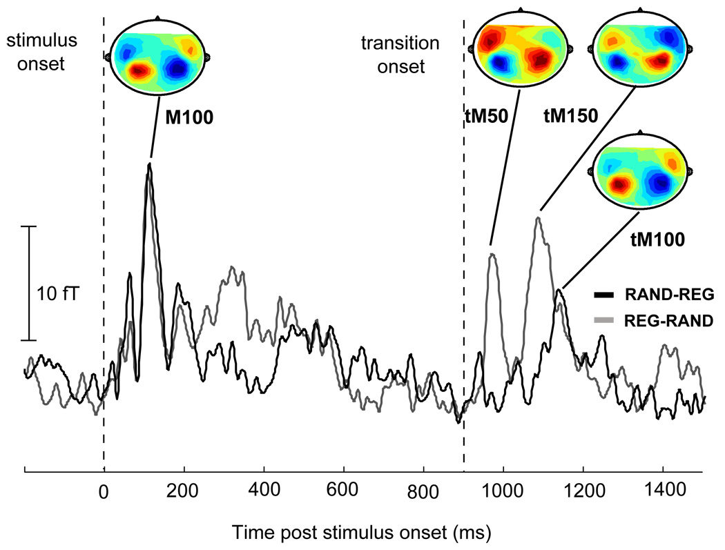
Measured data in the Random↔Regular block: Root mean square (RMS) of the grand-average (average over all subjects for each of the 156 channels) of the evoked auditory cortical responses to RAND-REG (in grey) and REG-RAND (in black) stimuli. Contour maps at the peaks are also provided; Source = red, Sink = blue. Onset response dynamics to CONST-REG and REG-CONST stimuli are identical. Both are characterized by a pronounced M100 onset response at approximately 110 ms post onset, with similar magnetic field distributions. Transition responses, however, differ greatly between REG-RAND and RAND-REG in both temporal dynamics and field distribution. The REG-RAND transition evokes a first deflection (tM50) peaking at about 70 ms post transition, with an M50-like magnetic field polarity, and another deflection (tM150) at about 180 ms post transition, also with an M50-like magnetic field pattern. The peak of the first response to the opposite (RAND-REG) transition (tM100) occurs at about 240 ms post transition, with an M100-like magnetic field polarity. All statistical analyses were performed on each-hemisphere, subject-by-subject (based on the 10 channels selected for each in each hemisphere). The grand-average plot is shown here for illustration purposes only.
Transition response
Unlike onset responses, transition responses exhibit clear response timing and response polarity differences between conditions. The transition from a constant tone to a regular sequence of tone pips evokes a first deflection peaking at about 70 ms post transition, with an M50-like magnetic field polarity (the MEG counterpart of the EEG P1 response), followed by another deflection at about 120 ms post transition, with an M100-like magnetic field polarity (the MEG counterpart of the EEG N1 response; Näätänen and Picton, 1987). These peaks will be referred to as ‘transition-evoked M50 response’ (tM50) and ‘transition-evoked M100 response’ (tM100) in the remainder of the manuscript. The first response to the opposite (REG-CONST) transition peaks at about 160 ms post transition, with an M100-like magnetic field pattern, followed by an additional deflection at about 250 ms post transition with an M150 dipolar distribution (the counterpart of the EEG P2 deflection). As above, these peaks will be referred to as tM100 and tM150.
The tM100 deflection, common to both transition directions, exhibited a significantly higher amplitude in the case of REG-CONST transitions (repeated measures ANOVA on peak amplitudes with hemisphere and transition direction as factors revealed only a main effect of transition direction F(1,11)=9.6 p=0.01) and occurred about 30 ms later than the opposite transition (repeated measured ANOVA on peak latencies with hemisphere and transition direction as factors revealed only a main effect of transition direction F(1,11)=31.8 p<0.0001).
Figure 3 presents the post-transition RMS activation time course in the left and right hemispheres for CONST-REG (Fig 3A, C) and REG-CONST (Fig 3B, D) transitions, as compared to their respective control (no change; CONST and REG, respectively) conditions. Grey shadings mark temporal intervals where a repeated measures bootstrap (see Methods) indicated a significant difference between transition (black) and control (grey) conditions. In the case of CONST-REG stimuli, the first difference from the control condition emerges at 46 ms post transition in the left hemisphere and 24 ms post transition in the right hemisphere. For REG-CONST stimuli, the first difference from the control condition is at 120 ms post transition in the left hemisphere and at 124 ms post transition in the right hemisphere. The figure also demonstrates the existence of a sustained response in CONST-REG stimuli, which commences at about 250 ms after the transition (the 1 Hz hardware high-pass filtering applied to responses recorded in this study probably causes an attenuation of these sustained responses, however they are visible even here). Such sustained responses (see also Gutschalk et al., 2004) seem to be a general property of fluctuating vs. constant signals and are also observed in signals such as uncorrelated vs. correlated noise (Chait et al., 2007b) for which the fluctuation is in the interaural-correlation domain, not in the frequency domain.
Figure 3.
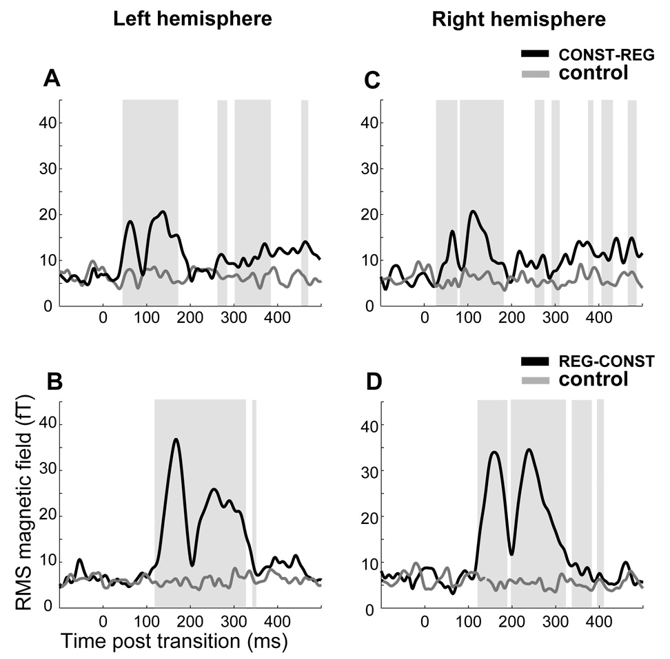
Transition responses in Constant↔Regular_stimuli. The plots illustrate the time points for which the ‘change’ conditions first diverge from their controls. A: grand-average RMS magnetic field of the CONST-REG transition (black) and its control (no change; CONST) in the left hemisphere. B: grand-average RMS magnetic field of the REG-CONST transition (black) and its control (no change; REG) in the left hemisphere. C: grand-average RMS magnetic field of the CONST-REG transition (black) and its control (no change; CONST) in the right hemisphere. D: grand-average RMS magnetic field of the REG-CONST transition (black) and its control (no change; REG) in the right hemisphere. Shaded areas mark time intervals where a significant difference is found between transition and control. Note that differences are computed in a repeated measures analysis and therefore may be marked as significant even when the grand-average RMS plot shows no difference between conditions.
As discussed in the Introduction, an ideal observer can immediately detect the transition in CONST-REG based on the frequency change occurring at the time of the transition (Fig 1). To detect the opposite transition (REG-CONST), the observer must wait one extra pip-duration (30 ms) after the nominal transition. In reality, the latency difference between the first peaks of each condition is longer - about 100 ms. However, it is important to note that the detection of the REG-CONST transition is not only delayed with respect to the CONST-REG transition, but also involves a different sequence of MEG deflections (tM50 and tM100 in the case of CONST-REG, and tM100 and tM150 in the case of REG-CONST). Distributions of opposite polarity most likely reflect the activation of at least partly distinct neural substrates (see below; Lütkenhöner, 2003; see also Jones, 2002) suggesting the involvement of partially different neural substrates in detecting the temporal edge, depending on the direction of change.
Random↔Regular edges
Magnetic waveform and field distribution analyses reveal that participants had comparable response trajectories. Figure 4 shows the root mean square (RMS) of the grand-averaged auditory evoked responses to random-to-regular (RAND-REG; in grey) and regular-to-random (REG-RAND; in black) edges. The origin of the time scale coincides with the onset of the signals and the transition occurs at 900 ms post stimulus onset. The evoked MEG activity exhibits a series of deflections at about 100 ms after stimulus onset and a later series of deflections after the transition that begin at about 970 ms post onset (70 ms post transition). These two aspects of the response are discussed, in turn, below.
Onset Response
Onset responses to both conditions had similar dynamics (latency and shape of the deflection) and magnetic field distributions. Specifically, both conditions produced a prominent onset response with a peak at approximately 110 ms post onset with a characteristic M100 field distribution (see Fig 4). Repeated measures ANOVAs on peak latencies and amplitudes, with hemisphere and condition as factors, revealed no significant differences.
Transition response
Unlike onset responses, which look qualitatively rather similar across conditions, transition responses differ greatly between REG-RAND and RAND-REG in both temporal dynamics and field distribution (Fig. 4). The transition from a regular to a random sequence of tone pips evokes a first deflection peaking at about 70 ms post transition, with an M50-like magnetic field polarity, and another deflection at about 180 ms post transition, also with an M50-like magnetic field pattern. As above, these peaks will be referred to as tM50 and tM150. The peak of the first response to the opposite (RAND-REG) transition occurs at about 240 ms post transition, with an M100-like magnetic field polarity and will be referred to as tM100.
Figure 5 presents the post-transition RMS activation time course in the left and right hemispheres for RAND-REG (Fig 5A, C) and REG-RAND (Fig 5B, D) transitions, as compared to their respective control (no change; RAND and REG, respectively) conditions. Grey shading marks temporal intervals where a repeated measures bootstrap (see Methods) indicated a significant difference between transition (black) and control (grey) conditions. In the case of RAND-REG stimuli, the first difference from the control condition emerges at 54 ms post transition in the left hemisphere and 60 ms post transition in the right hemisphere. For REG-CONST stimuli, the first difference from the control condition is at 203 ms post transition in the left hemisphere and at 218 ms post transition in the right hemisphere.
Figure 5.
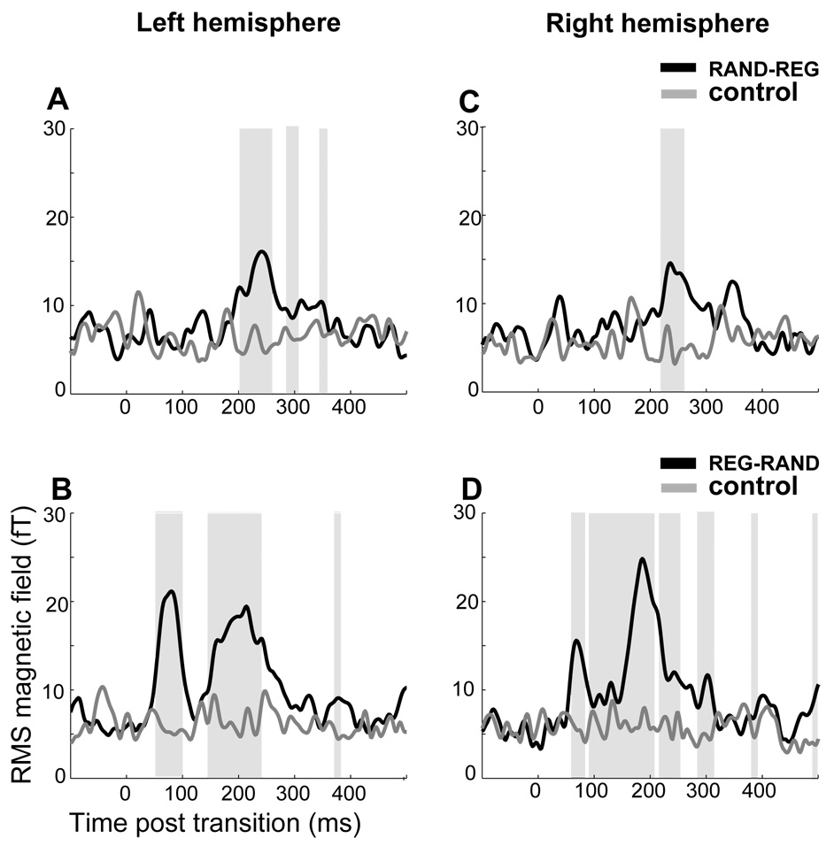
Transition responses in Constant↔Regular_stimuli. The plots illustrate the time points for which the ‘change’ conditions first diverge from their controls. A: grand-average RMS magnetic field of the RAND-REG transition (black) and its control (no change; RAND) in the left hemisphere. B: grand-average RMS magnetic field of the REG-RAND transition (black) and its control (no change; REG) in the left hemisphere. C: grand-average RMS magnetic field of the RAND-REG transition (black) and its control (no change; RAND) in the right hemisphere. D: grand-average RMS magnetic field of the REG-RAND transition (black) and its control (no change; REG) in the right hemisphere. Shaded areas mark time intervals where a significant difference is found between transition and control. Note that differences are computed in a repeated measures analysis and therefore may be marked as significant even when the grand-average RMS plot shows no difference between conditions.
The dipolar distribution of the first (tM50) peak in the REG-RAND transition is of opposite polarity from that of the first peak in RAND-REG transition (tM100; Fig 4), indicating that the underlying currents flow in opposite directions. Such a difference may be due to different neural sources, a difference in excitatory vs. inhibitory currents, or both. The sources underlying these two dipolar patterns are too close to be adequately differentiated with the spatial resolution of our recording technique. However, given that measurable magnetic fields are principally produced by dendritic currents in pyramidal neurons (Nunez and Silberstein, 2000) distributions of opposite polarity most likely reflect the activation of at least partially distinct neural substrates (Lutkenhoner, 2003; see also Jones, 2002). Therefore, the response to the RAND-REG transition is not only delayed (as discussed in the introduction) with respect to that of the REG-RAND transition, but also appears to involve at least partly different neural populations (see also Chait et al., 2007a), and interpreted as indicating that different neural mechanisms are involved in processing the two types of transitions.
The responses to the RAND-REG transition are distinctly noisier than the other transitions reported here (Fig 3, Fig 5). This is demonstrated in Figure 6, where, for each transition condition, we plot the standard deviation (across subjects) of first peak latency in the left and right hemispheres. It is probably the case that the timing of the peak in this case is strongly influenced by the particular pattern in the RAND segment preceding the transition (as well as each listener’s specific strategy for deciding when there has been enough evidence accumulated to signal a transition). This was not controlled in the present study and would be an interesting avenue for further investigation.
Figure 6.
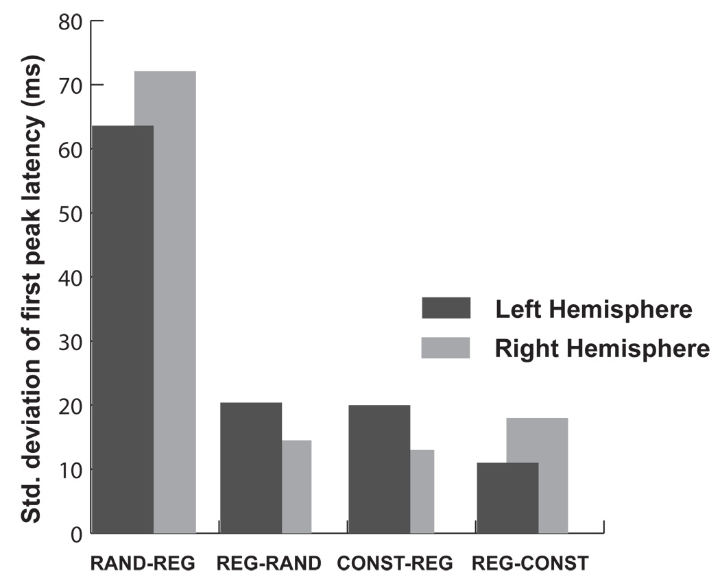
Standard deviation (across subjects) of first peak latency. Dark bars: left hemisphere, light bars: right hemisphere.
Discussion
The emergence of an object within a background is often signaled by the existence of edges, or transitions in the properties of the stimulus as one moves (in space for a visual scene, in time for an auditory scene) across the sensory map. The experiment described here used MEG because of its compelling sensitivity for human auditory cortical activity, in particular in the time domain, to probe a hypothesized process that may lie at the basis of auditory scene analysis – temporal edge detection. The present data extend previous MEG findings (Chait et al., 2005; Chait et al., 2007a) over a wider range of stimuli allowing to draw stronger conclusions. We demonstrate that the temporal dynamics and morphology of the neural temporal-edge-detection responses depend in precise ways on the nature of the edge (the context before and after the transition).
To the extent that response latencies may be indicative of the areas activated (see e.g. discussion in Krumbholz et al., 2007; Haenschel etl al, 2005), the onset latency of the tM50 component (about 20–60 ms post transition, depending on the stimulus; see Fig 3, Fig 5) suggests that its generators are likely lying in the medial to lateral extent of Heschl’s gyrus, inside or near primary (core) auditory cortex (Liegeois-Chauvel et al., 1991; Liegeois-Chauvel et al, 1994; Yvert et al., 2001). The latency of the tM100 response implicates generators in non-primary auditory cortex: lateral Heschl’s gyrus and planum temporale (Krumbholz et al., 2003; Godey et al., 2001; Lütkenhöner and Steinsträter, 1998).
These results suggest that distinct neural substrates in putative primary and non-primary auditory cortex are recruited depending on the kind of computation required to extract the edge, specifically the detection of a deviation from a previously encoded invariant feature of the acoustic environment versus the discovery of the emergence of a new invariant feature (see below).
Relationship to the MMN
These findings relate to but are distinct from the MMN change-detection response (Näätänen et al., 1978; Kujala and Näätänen, 2003; Polich, 2003). The earliest transition-related responses that we observe occur with significantly shorter latencies than typical MMN responses, and with specific, edge-dependent, temporal/morphological dynamics that are not usually found in MMN studies.
It is quite possible (and even plausible) that some generators are common to the two types of responses (specifically the later peaks we observe; see also Jones, 2002). MMN-generators, detecting a discrepancy between the preceding context and the new, deviant, information, may be contributing to responses to REG-CONST transitions, where there is a duration change with regard to the events in the preceding 900 ms segment, and to CONST-REG and REG-RAND signals, where there is a frequency change at the transition.
Several recent studies have tested transitions from a random sequence to repetition within the MMN paradigm framework (Horváth et al., 2001; Wolff and Schröger, 2001; Näätänen and Rinne, 2002; Horváth and Winkler, 2004): Occasional repetitions of a tone within a sequence of tones of random frequency has been shown to elicit an MMN like negativity (sometimes termed ‘repetition negativity’, RN) that peaks about 100–200 ms after the onset of repetition. The RN has been interpreted to reflect the fact that auditory cortex is able to extract ‘frequency variation’ as an invariant feature of the acoustic environment (Wolff and Schröger, 2001; Horváth and Winkler, 2004). Others (Näätänen and Rinne, 2002) have argued that the RN does not reflect an MMN process but is generated by neural activity forming a longer-duration memory trace of the repeating stimulus. Because of the differences between the present, ‘transition-response’, stimulus configuration and the MMN paradigm, based on randomly interleaved standards and deviants, it is not straightforward to compare these results with the responses obtained in the present study. We note, however, that the RAND-REG edge, to the best of our knowledge used here for the first time, is an example of a transition that is the opposite of an MMN-eliciting stimulus configuration: This transition does not violate any preceding regularity and is instead characterized by the emergence of regularity out of disorder. Consequently the elicited cascade of responses must, by definition, be distinct from the canonical MMN.
The term ‘emergence of regularity’, in this context, can have two, somewhat different, meanings. The first is related to the process of acquiring a specific deterministic rule about the succession of elements in a pattern. The second is related to the detection of some transition in the pattern of the statistics (e.g. mean, variance, etc) of the features of an ongoing sound (e.g. Deweese and Zador, 1998). For instance, variability in possible frequency steps between two successive pips, which is higher in the RAND than in the REG condition, may be sufficient to detect a transition without relying on the detection of the regularity rule used to generate the sounds. The way in which our stimuli were presented to the listeners (blocked by stimulus type) does not allow to differentiate the two sorts of processes - in this kind of stimulus presentation we can think of the ‘regularity rule’ as being already formed and the task faced by the auditory system is to decide whether and when to activate it, depending on the properties of the ongoing input. Indeed it is likely that the responses we observe in the RAND-REG transition reflect this kind of process.
Acoustic temporal edge detection
Stimulus configurations similar to the ones in the present study have been used in the literature to investigate auditory cortical processing of various kinds of acoustic features (e.g. Lavikainen et al., 1995; Kaernbach et al., 1998; Martin and Boothroyd, 2000; Jones and Perez, 2002; Krumbholz et al, 2003; Ross et al, 2004; Gutschalk et al., 2004; Chait et al., 2006; Ross et al., 2007). By measuring responses to transitions between a baseline signal and a test signal (differing from the baseline signal by a feature of interest), these studies attempt to tap processing specific to the test feature, distinct from the mechanisms responding to stimulus energy onset. Our results suggest a somewhat different approach to the interpretation of these transition responses as reflecting the detection of ‘auditory temporal edges’. For example, recent MEG studies measuring responses to disorder/order transitions between irregular and regular click trains (Gutschalk et al., 2004) or between white noise and iterated rippled noise (IRN; Krumbholz et al., 2003; Rupp et al., 2005), collectively labeled in the literature as the pitch onset response and hypothesized to reflect cortical pitch processing mechanisms, report responses that bare a similarity to the asymmetries observed here for transitions between random and regular sequences of tone pips (RAND-REG stimuli). Specifically, transitions from white noise to IRN evoked one peak with a M100 field distribution while the opposite transition (form IRN to noise) evokes instead two prominent M50 and M150 responses (Rupp et al., 2005). Indeed it is possible to describe the shift between noise and IRN as a transition between states that differ along a more abstract dimension, such as degree of regularity or order, and the pitch onset response may thus not reflect pitch processing per se, but mechanisms, such as those described in the present manuscript, that handle changes in the pattern of ongoing input statistics.
Auditory cortical mechanisms of temporal edge detection
Our data reveal a functional dissociation between the transition-evoked M50 (generally considered to be the MEG counterpart of the P1 EEG response) and M100 (generally considered to be the MEG counterpart of the N1 EEG response) responses (labeled here as tM50 and tM100 to distinguish them from onset responses), which are often treated in the literature as a unitary activation sequence, evoked by sound onset: We demonstrate response configurations (REG-RAND transitions) in which a tM50 response appears without a following tM100 response, others (RAND-REG and REG-CONST transition) in which an M100 response appears without a preceding tM50 deflection, and also evoked field patterns in which both responses are observable (CONST-REG transitions). (See also Jones (2002), for some additional evidence for a dissociation of these responses, based on data from comatose-patients.)
What processes do these deflections reflect? Although some of the response characteristics we describe (e.g. amplitudes) may be attributed to physical stimulus differences (i.e. REG vs. CONST vs. RAND), we demonstrate that the existence or non-existence of particular MEG deflections is correlated with certain abstract characteristics of the transition. The different sequence of activations, depending on the properties of the edge, enables access to the functional role of the mechanisms generating the measured cortical activations. Early transition-evoked tM50 responses, probably originating from in or near primary auditory cortex (Liegeois-Chauvel et al., 1991; Liegeois-Chauvel et al., 1994; Yvert et al., 2001), are observed in situations in which the auditory edge consists of an immediate stepwise change in some, previously constant, stimulus property like a transition in frequency (e.g. CONST-REG and REG-RAND stimuli in the present study; Chait et al., 2007a; Jones et al., 2002; Martin and Boothroyd 2000), change in interaural phase difference (Ross et al., 2007), change from correlated to uncorrelated noise (Chait et al., 2005; Chait et al., 2007b), transition between iterated rippled noise segments of different pitch (Ritter et al., 2005) or for transitions between iterated rippled noise and white noise (Rupp et al., 2005).
tM100 responses, without an observable preceding tM50 response, seem to occur for disorder-to-order type auditory edges, where a previously irregular stimulus feature begins to alternate regularly: e.g. transitions between random and regular sequence of tone pips (RAND-REG in this study), transitions between a random sequence of tone pips to a constant tone (Chait et al., 2007a; Jones, 2002), transitions from uncorrelated to correlated noise (Chait et al., 2005; Chait et al., 2007b), from white noise to iterated rippled noise (Krumbholz et al., 2003; Rupp et al., 2005; Seither-Preisler et al., 2005), or from an irregular sequence of click trains to a regular one (Gutschalk et al., 2004). The latency of this deflection, which appears to originate in higher order auditory cortex (Godey et al., 2001; Lütkenhöner and Steinsträter., 1998), varies in precise ways depending on the properties of the edge (e.g. Krumbholz et al., 2003; Chait et al., 2007a) and is a cue to how long it takes to detect the particular pattern change of ongoing statistics. More research into these features may provide the key to a better understanding of the computations that govern these processes and how different kinds of regularities are represented in auditory cortex.
A combination of tM50 and tM100 responses is observed in situations in which the transition is between two regular signals, such that processing of the edge is a combination of discovering a deviation from the previous regularity, and the detection of a predictability in the new pattern: e.g. transitions between two constant tones (Chait et al., 2007a), between a constant tone and a regularly alternating sequence of tones (CONST-REG in the present study), between two tones with different interaural phase difference (Ross et al., 2007), between iterated rippled noise segments of different pitch (Ritter et al., 2005). It is noteworthy that the REG-CONST transition in the present study did not evoke a tM50 response as would be expected under such an interpretation. An explanation of this may be that the neural mechanisms underlying the transition-evoked M50 response are limited by the kinds of violations of regularity that they can compute, and the kind of violation of regularity that characterizes the transition between REG and CONST (a B tone that fails to follow the A tone) is not detectable by these mechanisms. The tM50 transition-response may be therefore reflecting the operation of relatively early sensory change detection mechanisms, for example based on differential states of refractoriness of neurons tuned to a particular basic feature (e.g. Opitz et al., 2005). Note that if this hypothesis is correct, then the occurrence of a tM50 response in a transition may be a tool for investigating what features of a regular event constitute ‘basic features’ that are represented by the early auditory cortical mechanisms that underlie the response.
The kinds of operations needed for detecting transitions from regular to irregular auditory patterns are conceptually different from those required for the detection of transitions in the opposite direction (from irregular to regular). In the former case one needs to detect a violation of a previously acquired regularity. In the latter case, the transition cannot be detected as a mere shift along a feature dimension: detection requires acquiring a representation of the statistics before the transition, comparing it with a representation of the statistics after the transition, and deciding whether the two are compatible with the absence of change, or instead indicate a transition. Here we show, based on the fact that regular-to-irregular and irregular-to-regular transitions evoke different sequences of MEG activations, that these operations do not differ only by the amount of integration time required to detect the transition but appear to recruit distinct neural substrates in core and non-core human auditory cortex.
The stimuli we used so far have been very simple instances of acoustic temporal edges. Additional limitations are that different kinds of stimuli were blocked separately and not interleaved in an ecologically relevant manner. The further investigation of these temporal-edge-evoked responses may provide a tool to measure what is deemed ‘regularity’ by the auditory system and a key for understanding what aspects of ongoing stimulus statistics the system is sensitive to, and how it estimates them - allowing new insight into the organization and representation of auditory objects in human auditory cortex.
Materials and Methods
Subjects
Twelve subjects (mean age 24.8 years, 4 female) participated in the experiment. All were right handed (Oldfield, 1971), reported normal hearing, and had no history of neurological disorder. The experimental procedures were approved by the University of Maryland institutional review board and written informed consent was obtained from each participant. Subjects were paid for their participation.
Stimuli
The experiment consisted of three successive blocks, each containing different stimuli (see below; the analysis of the data for one of the blocks is constrained by a technical difficulty and therefore data from only two experimental blocks are reported here). Block order was counter-balanced across subjects. Figure 1 describes the stimuli used in the two blocks reported here. The frequencies for all patterns were drawn randomly from a frequency set of 19 values spaced in 12% steps between 222 and 1781 Hz. All tonal transitions were ramped on and off with 3 ms raised-cosine ramps.
In addition to the tonal stimuli the stimulus set in each block included a proportion (33%, or 240 per block) of wide-band noise bursts of duration 200 ms with 10 ms raised-cosine onset and offset ramps. These decoy stimuli were delivered between the test sounds and subjects were instructed to detect them. This task served to insure that subjects remained vigilant and attentive to the auditory modality, but did not require any processing of the tonal changes that were the focus of our study.
The stimuli were created off-line and saved in 16-bit stereo wave format at a sampling rate of 44 kHz. The signals were delivered to the subjects’ ears with tubephones (E-A-RTONE 3A 50 ohm, Etymotic Research, Inc) attached to E-A-RLINK foam plugs inserted into the ear-canal and presented at a comfortable listening level. The inter-stimulus interval (ISI) was randomized between 600–1400 ms.
Constant↔Regular edges (Fig 1A)
Stimuli were 1530 ms in duration and consisted of a pure tone modulated in frequency and amplitude according to 4 patterns (CONST, REG, CONST-REG, REG-CONST). CONST and REG stimuli served as controls for the CONST-REG and REG-CONST stimuli.
The REG signals consisted of a regularly alternating sequence of three 30 ms tone pips (A, B and C). The frequencies of A, B and C were drawn randomly from the above frequency pool as three consecutive frequency steps and their order was permuted before assignment to A, B and C. The CONST stimulus was a pure tone whose frequency was randomly drawn from the above frequency set. The REG-CONST stimulus consisted of an initial 900 ms REG segment (10 repetitions of an ABC triplet) followed by a 630 ms post-transition segment which consisted of a pure tone with frequency A. The CONST-REG stimulus contained an initial 900 ms pure tone with a constant frequency followed by a 630 ms post-transition REG segment. CONST-REG and REG-CONST stimuli were initially created as mirror images of each other, and then trimmed to the required duration.
We generated 40 signals for each of the 4 patterns (CONST, REG, CONST-REG, REG-CONST). Subjects heard 120 repetitions of every one of the 4 patterns and the order of presentation was randomized.
Random↔Regular edges (Fig 1B)
Stimuli were 1530 ms in duration and consisted of a pure tone modulated in frequency and amplitude according to 4 patterns (RAND, REG, RAND-REG, REG-RAND). RAND and REG stimuli served as controls for the RAND-REG and REG-RAND stimuli.
The REG stimulus was as defined above. The RAND stimulus consisted of a sequence of 30 ms tone pips, with frequencies drawn randomly from the above set of 19 values. The REG-RAND stimulus contained an initial 900 ms REG segment (10 repetitions of an ABC triplet) followed by a 630 ms post-transition RAND segment (21 random frequency tone pips). The RAND-REG stimulus consisted of an initial 900 ms RAND segment followed by a 630 ms post-transition REG segment. To control for frequency content and step-size at the transition, RAND-REG and REG-RAND stimuli were initially created as mirror images of each other, and then trimmed to the required duration.
We generated 40 signals for each of the 4 patterns (RAND, REG, RAND-REG, REG-RAND). Subjects heard 120 repetitions of every one of the 4 patterns and the order of presentation was randomized.
Procedure
Subjects lay supine inside a magnetically shielded room. The experimental session included two phases: a preliminary functional source-localizer recording, followed by the main experiment. In the functional source-localizer recording subjects listened to 200 repetitions of a 1 kHz 50 ms sinusoidal tone (ISI randomized between 750–1550 ms). These responses were used to verify that the subject was positioned properly in the machine, that signals from auditory cortex had a satisfactory signal to noise ratio (SNR) and to determine which MEG channels best respond to activity within auditory cortex.
In the main experiment (about 1.5 hours duration), subjects listened to stimuli while performing the noise burst detection task as described above. They were instructed to respond by pressing a button, held in the right hand, as soon as a noise burst appeared. The instructions encouraged speed and accuracy. The presentation was divided into runs of 180 stimuli (4 runs per stimulus block). Between runs, subjects were allowed a short rest but were required to stay still.
Neuromagnetic recording and data analysis
Methods and analysis are described in more detail in Chait et al. (2005). The magnetic signals were recorded using a 160-channel, whole-head axial gradiometer system (KIT, Kanazawa, Japan). Data for the localizer recording were acquired with a sampling rate of 1 kHz, filtered online between 1 Hz (hardware filter) and 58.8 Hz (17 ms moving average filter), stored in 500 ms stimulus-related epochs starting 100 ms pre-onset, and baseline-corrected to the 100 ms pre-onset interval. The M100 onset response (Hari, 1990; Roberts et al., 2000) was identified for each subject as a dipole-like pattern (i.e. a source/sink pair) in the magnetic field contour plots distributed over the temporal region of each hemisphere. The M100 current source is quite robustly localized to the upper banks of the superior temporal gyrus in both hemispheres (Hari, 1990; Pantev et al., 1995; Lütkenhöner and Steinsträter, 1998). For each subject, the 20 strongest channels at the peak of the M100 (5 in each sink and source, yielding 10 in each hemisphere) were considered to best reflect activity in the auditory cortex and thus chosen for the analysis of the experimental data. This procedure serves the dual purpose of enhancing the auditory response components over other response components, and compensating for any channel-misalignment between subjects.
Data for the main experiment were acquired continuously with a sampling rate of 0.5 kHz, filtered in hardware between 1 and 200 Hz with a notch at 60 Hz (to remove line noise). Offline, the data were noise-reduced using the Time-Shift Principle Component Analysis algorithm (TSPCA; de Cheveigné and Simon, 2007) and then smoothed by convolution with a 39 ms Hanning window (cutoff 55 Hz). 1600 ms epochs (including 200 ms pre onset) were created for each of the eight stimulus conditions (2 blocks × 4 patterns). Epochs with amplitudes larger than 3 pT (<5%) were considered artifactual and discarded. The rest were averaged. In each hemisphere, the root mean square (RMS) of the field strength across the 10 channels, selected in the functional source-localizer run, was calculated for each sample point. Sixteen RMS time series, one for each condition in each hemisphere, were thus created for each subject.
Two measures of the dynamics of brain response are reported: the time course of the RMS, reflecting instantaneous amplitude of neural responses, and the spatial distributions of the magnetic field (contour plots), sampled at certain times post onset. The congruity of activation time course and magnetic field distributions across subjects were evaluated using the bootstrap method (Efron and Tibshirani, 1993; 500 iterations; balanced) based on the individual RMS time series as described in Chait et al. (2007a). For illustration purposes, we plot an RMS of the grand-average (average over all subjects) but statistical analysis is always performed on a subject by subject, hemisphere by hemisphere, basis, using the RMS over the 10 channels chosen for each subject in each hemisphere.
To compare the activation between conditions, we used a repeated measures analysis in which, for each subject, the squared RMS value of one condition is subtracted from the squared RMS value of the other condition and the individual difference time series are subjected to a bootstrap analysis (500 iterations; balanced; Efron and Tibshirani, 1993). At each time point, the proportion of iterations below the zero line is counted. If that proportion is less than 1%, or more than 99% for 5 adjacent samples (10 ms) and if the average absolute difference at that time exceeded a threshold of 200 fT2 the difference is judged to be significant.
Peak latencies and amplitudes for the ANOVA tests were computed by selecting, for each subject, the maximum value within the relevant time window, which was defined as ±20ms centered around the grand-average RMS peak. The α level was set, a-priori, to 0.05.
Acknowledgements
We are grateful to Jeff Walker for excellent technical support and to Alain de Cheveigné for comments and discussion. This research was supported by NIH grant R01DC05660 to DP and European grant IST Project FP6-03773 to École Normale Supérieure, Paris, France.
Footnotes
Publisher's Disclaimer: This is a PDF file of an unedited manuscript that has been accepted for publication. As a service to our customers we are providing this early version of the manuscript. The manuscript will undergo copyediting, typesetting, and review of the resulting proof before it is published in its final citable form. Please note that during the production process errors may be discovered which could affect the content, and all legal disclaimers that apply to the journal pertain.
References
- Adachi Y, Shimogawara M, Higuchi M, Haruta Y, Ochiai M. Reduction of non-periodic environmental magnetic noise in MEG measurement by continuously adjusted least squares method. IEEE Transactions on Applied Superconductivity. 2001;11:669–672. [Google Scholar]
- Burr DC, Morrone MC, Spinelli D. Evidence for edge and bar detectors in human vision. Vision Res. 1989;29:419–431. doi: 10.1016/0042-6989(89)90006-0. [DOI] [PubMed] [Google Scholar]
- Chait M, Poeppel D, de Cheveigné A, Simon JZ. Human auditory cortical processing of changes in interaural correlation. J Neurosci. 2005;25:8518–8527. doi: 10.1523/JNEUROSCI.1266-05.2005. [DOI] [PMC free article] [PubMed] [Google Scholar]
- Chait M, Poeppel D, Simon JZ. Neural response correlates of detection of monaurally and binaurally created pitches in humans. Cereb Cortex. 2006;16:835–848. doi: 10.1093/cercor/bhj027. [DOI] [PubMed] [Google Scholar]
- Chait M, Poeppel D, de Cheveigné A, Simon JZ. Processing Asymmetry of Transitions between Order and Disorder in Human Auditory Cortex. J Neurosci. 2007a;27:5207–5214. doi: 10.1523/JNEUROSCI.0318-07.2007. [DOI] [PMC free article] [PubMed] [Google Scholar]
- Chait M, Poeppel D, Simon JZ. Stimulus context affects auditory cortical responses to changes in interaural correlation. J Neurophysiol. 2007b;98:224–231. doi: 10.1152/jn.00359.2007. [DOI] [PubMed] [Google Scholar]
- de Cheveigné A, Simon JZ. Denoising based on Time-Shift PCA. J Neurosci. Methods. 2007;165:297–305. doi: 10.1016/j.jneumeth.2007.06.003. [DOI] [PMC free article] [PubMed] [Google Scholar]
- Denham SL, Winkler I. The role of predictive models in the formation of auditory streams. J Physiol Paris. 2006;100:154–170. doi: 10.1016/j.jphysparis.2006.09.012. [DOI] [PubMed] [Google Scholar]
- DeWeese M, Zador A. Asymmetric dynamics in optimal variance adaptation. Neural Computation. 1998;10:1179–1202. [Google Scholar]
- Efron B, Tibshirani RJ. An introduction to the Bootstrap. NY, NY, USA: Chapman and Hall; 1993. [Google Scholar]
- Fishbach A, Nelken I, Yeshurun Y. Auditory edge detection: a neural model for physiological and psychoacoustical responses to amplitude transients. J Neurophysiol. 2001;85:2303–2323. doi: 10.1152/jn.2001.85.6.2303. [DOI] [PubMed] [Google Scholar]
- Godey B, Schwartz D, de Graaf JB, Chauvel P, Liegeois-Chauvel C. Neuromagnetic source localization of auditory evoked fields and intracerebral evoked potentials: a comparison of data in the same patients. Clin Neurophysiol. 2001;112:1850–1859. doi: 10.1016/s1388-2457(01)00636-8. [DOI] [PubMed] [Google Scholar]
- Grimm S, Roeber U, Trujillo-Barreto NJ, Schroger E. Mechanisms for detecting auditory temporal and spectral deviations operate over similar time windows but are divided differently between the two hemispheres. Neuroimage. 2006;32:275–282. doi: 10.1016/j.neuroimage.2006.03.032. [DOI] [PubMed] [Google Scholar]
- Gutschalk A, Patterson RD, Scherg M, Uppenkamp S, Rupp A. Temporal dynamics of pitch in human auditory cortex. Neuroimage. 2004;22:755–766. doi: 10.1016/j.neuroimage.2004.01.025. [DOI] [PubMed] [Google Scholar]
- Haenschel C, Vernon DJ, Dwivedi P, Gruzelier JH, Baldeweg T. Event-related brain potential correlates of human auditory sensory memory-trace formation. J Neurosci. 2005;25:10494–10501. doi: 10.1523/JNEUROSCI.1227-05.2005. [DOI] [PMC free article] [PubMed] [Google Scholar]
- Hari R. The neuromagnetic method in the study of the human auditory cortex. In: Grandori F, et al., editors. Auditory evoked magnetic fields and the electric potentials. Krager-Verlag: Basel; 1990. pp. 222–282. [Google Scholar]
- Herdener M, Esposito F, Di Salle F, Lehmann C, Bach DR, Scheffler K, Seifritz E. BOLD correlates of edge detection in human auditory cortex. Neuroimage. 2007;36:194–201. doi: 10.1016/j.neuroimage.2007.01.050. [DOI] [PubMed] [Google Scholar]
- Horváth J, Czigler I, Sussman E, Winkler I. Simultaneously active pre-attentive representations of local and global rules for sound sequences. Cognitive Brain Research. 2001;12:131–144. doi: 10.1016/s0926-6410(01)00038-6. [DOI] [PubMed] [Google Scholar]
- Horváth J, Winkler I. How the human auditory system treats repetition amongst change. Neuroscience Letters. 2004;368:157–161. doi: 10.1016/j.neulet.2004.07.004. [DOI] [PubMed] [Google Scholar]
- Hubel DH, Wiesel TN. Receptive fields and functional architecture in two nonstriate visual areas (18 and 19) of the cat. J Neurophysiol. 1965;28:229–289. doi: 10.1152/jn.1965.28.2.229. [DOI] [PubMed] [Google Scholar]
- Jones SJ. The internal auditory clock: what can evoked potentials reveal about the analysis of temporal sound patterns, and abnormal states of consciousness? Neurophysiol Clin. 2002;32:241–253. doi: 10.1016/s0987-7053(02)00309-x. [DOI] [PubMed] [Google Scholar]
- Jones SJ, Perez N. The auditory C-process of spectral profile analysis. Clin Neurophysiol. 2002;113:1558–1565. doi: 10.1016/s1388-2457(02)00219-5. [DOI] [PubMed] [Google Scholar]
- Julesz B. Visual pattern discrimination. IEEE Transactions on Information Theory. 1962;8:84–92. [Google Scholar]
- Kaernbach C, Schroger E, Gunter TC. Human event-related brain potentials to auditory periodic noise stimuli. Neurosci Lett. 1998;242:17–20. doi: 10.1016/s0304-3940(98)00034-2. [DOI] [PubMed] [Google Scholar]
- Krumbholz K, Patterson RD, Seither-Preisler A, Lammertmann C, Lütkenhöner B. Neuromagnetic evidence for a pitch processing center in Heschl's gyrus. Cereb Cortex. 2003;13:765–772. doi: 10.1093/cercor/13.7.765. [DOI] [PubMed] [Google Scholar]
- Krumbholz K, Hewson-Stoate N, Schonwiesner M. Cortical response to auditory motion suggests an asymmetry in the reliance on inter-hemispheric connections between the left and right auditory cortices. J Neurophysiol. 2007;97:1649–1655. doi: 10.1152/jn.00560.2006. [DOI] [PubMed] [Google Scholar]
- Kujala A, Näätänen R. Auditory environment and change detection as indexed by the mismatch negativity (MMN) In: Polich J, editor. Detection of change: event related potential and fMRI findings. Boston, USA: Kluwer academic publishers; 2003. pp. 1–22. [Google Scholar]
- Lamme VA, Rodriguez-Rodriguez V, Spekreijse H. Separate processing dynamics for texture elements, boundaries and surfaces in primary visual cortex of the macaque monkey. Cereb Cortex. 1999;9:406–413. doi: 10.1093/cercor/9.4.406. [DOI] [PubMed] [Google Scholar]
- Lavikainen J, Huotilainen M, Ilmoniemi RJ, Simola JT, Näätänen R. Pitch change of a continuous tone activates two distinct processes in human auditory cortex: a study with whole-head magnetometer. Electroencephalogr Clin Neurophysiol. 1995;96:93–96. doi: 10.1016/0013-4694(94)00283-q. [DOI] [PubMed] [Google Scholar]
- Liegeois-Chauvel C, Musolino A, Chauvel P. Localization of the primary auditory area in man. Brain. 1991;114:139–151. [PubMed] [Google Scholar]
- Liegeois-Chauvel C, Musolino A, Badier JM, Marquis P, Chauvel P. Evoked potentials recorded from the auditory cortex in man: evaluation and topography of the middle latency components. Electroencephalogr Clin Neurophysiol. 1994;92:204–214. doi: 10.1016/0168-5597(94)90064-7. [DOI] [PubMed] [Google Scholar]
- Lütkenhöner B, Steinsträter O. High-precision neuromagnetic study of the functional organization of the human auditory cortex. Audiol. Neurootol. 1998;3:191–213. doi: 10.1159/000013790. [DOI] [PubMed] [Google Scholar]
- Lütkenhöner B. Magnetoencephalography and its Achilles' heel. J Physiol Paris. 2003;97:641–658. doi: 10.1016/j.jphysparis.2004.01.020. [DOI] [PubMed] [Google Scholar]
- Marr D, Hildreth E. Theory of edge detection. Proc R Soc Lond B Biol Sci. 1980;207:187–217. doi: 10.1098/rspb.1980.0020. [DOI] [PubMed] [Google Scholar]
- Martin BA, Boothroyd A. Cortical, auditory, evoked potentials in response to changes of spectrum and amplitude. J Acoust Soc Am. 2000;107:2155–2161. doi: 10.1121/1.428556. [DOI] [PubMed] [Google Scholar]
- Moore BCJ, Glasberg BR. Suggested formulae for calculating auditory-filter bandwidths and excitation patterns. J. Acoust. Soc. Am. 1983;74:750–753. doi: 10.1121/1.389861. [DOI] [PubMed] [Google Scholar]
- Näätänen R, Gaillard AWK, Mäntysalo S. Early selective attention effect on evoked potential reinterpreted. Acta Psychologica. 1978;42:313–329. doi: 10.1016/0001-6918(78)90006-9. [DOI] [PubMed] [Google Scholar]
- Näätänen R, Picton T. The N1 wave of the human electric and magnetic response to sound: a review and an analysis of the component structure. Psychophysiology. 1987;24:375–425. doi: 10.1111/j.1469-8986.1987.tb00311.x. [DOI] [PubMed] [Google Scholar]
- Näätänen R. Attention and brain function. Hillsdale, NJ, USA: Lawrence Erlbaum Associates; 1992. [Google Scholar]
- Näätänen R, Winkler I. The concept of auditory stimulus representation in cognitive neuroscience. Psychol Bull. 1999;125:826–859. doi: 10.1037/0033-2909.125.6.826. [DOI] [PubMed] [Google Scholar]
- Näätänen R, Jacobsen T, Winkler I. Memory-based or afferent processes in mismatch negativity (MMN): a review of the evidence. Psychophysiology. 2005;42:25–32. doi: 10.1111/j.1469-8986.2005.00256.x. [DOI] [PubMed] [Google Scholar]
- Näätänen R, Rinne T. Electric brain response to sound repetition in humans: an index of long-term memory-trace formation? Neurosci. Lett. 2002;318:49–51. doi: 10.1016/s0304-3940(01)02438-7. [DOI] [PubMed] [Google Scholar]
- Nunez PL, Silberstein RB. On the relationship of synaptic activity to macroscopic measurements: does co-registration of EEG with fMRI make sense? Brain Topogr. 2000;13:79–96. doi: 10.1023/a:1026683200895. [DOI] [PubMed] [Google Scholar]
- Oldfield RC. The assessment and analysis of handedness: The Edinburgh inventory. Neuropsychologia. 1971;9:97–113. doi: 10.1016/0028-3932(71)90067-4. [DOI] [PubMed] [Google Scholar]
- Opitz B, Schroger E, von Cramon DY. Sensory and cognitive mechanisms for preattentive change detection in auditory cortex. Eur J Neurosci. 2005;21:531–535. doi: 10.1111/j.1460-9568.2005.03839.x. [DOI] [PubMed] [Google Scholar]
- Pantev C, Bertrand O, Eulitz C, Verkindt C, Hampson S, Schuierer G, Elbert T. Specific tonotopic organizations of different areas of the human auditory cortex revealed by simultaneous magnetic and electric recordings. Electroencephalogr Clin Neurophysiol. 1995;94:26–40. doi: 10.1016/0013-4694(94)00209-4. [DOI] [PubMed] [Google Scholar]
- Picton TW, Alain C, Otten L, Ritter W, Achim A. Mismatch negativity: different water in the same river. Audiol Neurootol. 2000;5:111–139. doi: 10.1159/000013875. [DOI] [PubMed] [Google Scholar]
- Plack CJ, Moore BCJ. Temporal window shape as a function of frequency and level. J. Acoust. Soc. Am. 1990;87:2178–2187. doi: 10.1121/1.399185. [DOI] [PubMed] [Google Scholar]
- Polich J. Detection of change: event related potential and fMRI findings. Boston, MA, USA: Kluwer academic press; 2003. [Google Scholar]
- Ritter S, Gunter Dosch H, Specht HJ, Rupp A. Neuromagnetic responses reflect the temporal pitch change of regular interval sounds. Neuroimage. 2005;27:533–543. doi: 10.1016/j.neuroimage.2005.05.003. [DOI] [PubMed] [Google Scholar]
- Roberts T, Ferrari P, Stufflebeam S, Poeppel D. Latency of the auditory evoked neuromagnetic field components: Stimulus dependence and insights towards perception. J Clin Neuropsychol. 2000;17:114–129. doi: 10.1097/00004691-200003000-00002. [DOI] [PubMed] [Google Scholar]
- Ross B, Herdman AT, Wollbrink A, Pantev C. Auditory cortex responses to the transition from monophonic to pseudo-stereo sound. Neurol Clin Neurophysiol. 2004;2004:18. [PubMed] [Google Scholar]
- Ross B, Tremblay KL, Picton TW. Physiological detection of interaural phase differences. J Acoust Soc Am. 2007;121:1017–1027. doi: 10.1121/1.2404915. [DOI] [PubMed] [Google Scholar]
- Rupp A, Uppenkamp S, Bailes J, Gutschalk A, Patterson RD. Time constants in temporal pitch extraction: A comparison of psychophysical and magnetic data. In: Pressnitzer D, de Cheveigné A, McAdams S, Collet L, editors. Auditory signal processing: physiology, psychoacoustics, and models. NY, NY, USA: Springer Verlag; 2005. pp. 119–125. [Google Scholar]
- Sams M, Hari R, Rif J, Knuutila J. The human auditory sensory memory trace persists about 10s: Neuromagnetic evidence. J. Cog. Neurosci. 1993;5:363–370. doi: 10.1162/jocn.1993.5.3.363. [DOI] [PubMed] [Google Scholar]
- Schonwiesner M, Novitski N, Pakarinen S, Carlson S, Tervaniemi M, Näätänen R. Heschl's gyrus, posterior superior temporal gyrus, and mid-ventrolateral prefrontal cortex have different roles in the detection of acoustic changes. J Neurophysiol. 2007;97:2075–2082. doi: 10.1152/jn.01083.2006. [DOI] [PubMed] [Google Scholar]
- Seither-Preisler A, Krumbholz K, Patterson R, Seither S, Lütkenhoner B. Interaction between the neuromagnetic responses to sound energy onset and pitch onset suggests common generators. Eur J Neurosci. 2004;19:3073–3080. doi: 10.1111/j.0953-816X.2004.03423.x. [DOI] [PubMed] [Google Scholar]
- Winkler I, Karmos G, Näätänen R. Adaptive modeling of the unattended acoustic environment reflected in the mismatch negativity event-related potential. Brain Res. 1996;742:239–252. doi: 10.1016/s0006-8993(96)01008-6. [DOI] [PubMed] [Google Scholar]
- Winkler I. Change detection in complex auditory environment: beyond the oddball paradigm. In: Polich J, editor. Detection of change: event related potential and fMRI findings. Boston, USA: Kluwer academic publishers; 2003. pp. 61–82. [Google Scholar]
- Winkler I. Interpreting the mismatch negativity (MMN) Journal of Psychophysiology. 2008 in press. [Google Scholar]
- Wolff C, Schroger E. Activation of the auditory pre-attentive change detection system by tone repetitions with fast stimulation rate. Brain Res Cogn Brain Res. 2001;10:323–327. doi: 10.1016/s0926-6410(00)00043-4. [DOI] [PubMed] [Google Scholar]
- Yvert B, Crouzeix A, Bertrand O, Seither-Preisler A, Pantev C. Multiple supratemporal sources of magnetic and electric auditory evoked middle latency components in humans. Cereb Cortex. 2001;11:411–423. doi: 10.1093/cercor/11.5.411. [DOI] [PubMed] [Google Scholar]