Population genetic analysis of shotgun assemblies of genomic sequences from multiple individuals

Abstract

We introduce a simple, broadly applicable method for obtaining estimates of nucleotide diversity θ from genomic shotgun sequencing data. The method takes into account the special nature of these data: random sampling of genomic segments from one or more individuals and a relatively high error rate for individual reads. Applying this method to data from the Celera human genome sequencing and SNP discovery project, we obtain estimates of nucleotide diversity in windows spanning the human genome and show that the diversity to divergence ratio is reduced in regions of low recombination. Furthermore, we show that the elevated diversity in telomeric regions is mainly due to elevated mutation rates and not due to decreased levels of background selection. However, we find indications that telomeres as well as centromeres experience greater impact from natural selection than intrachromosomal regions. Finally, we identify a number of genomic regions with increased or reduced diversity compared with the local level of human–chimpanzee divergence and the local recombination rate.

The nature of population genetic data has changed dramatically over the past few years. For the past 15–20 yr the standard data were Sanger sequenced DNA from one or a few genes or genomic regions, microsatellite markers, AFLPs, or RFLPs. With the availability of new high-throughput genotyping and sequencing technologies, large genome-wide data sets are becoming increasingly available. The focus of this article is the analysis of tiled population genetic data, i.e., data obtained as many small reads of DNA sequences that align relatively sparsely to a reference genome sequence or in segmental assemblies. These data differ from classical sequence data in several ways. The main difference is that for each nucleotide position under scrutiny, a different set of chromosomes is sampled. While this problem is similar to the usual missing data problem in directly sequenced data, it is different for diploid organisms, because it is unknown how many chromosomes from an individual are represented in any segment of the assembly. This implies that for any particular segment of the alignment it is not known whether aligned sequence reads are drawn from one or both chromosomes. The main objective of this study is to develop and apply statistics for addressing these problems. We will primarily do this in the framework of composite likelihood estimators (CLEs). CLEs are becoming popular for dealing with large-scale data in population genetics. They form the basis for a number of recent methods for analyzing large-scale population genetic data, including methods for estimating changes in population size (e.g., Nielsen 2000; Wooding and Rogers 2002; Polanski and Kimmel 2003; Adams and Hudson 2004; Myers et al. 2005) and methods for quantifying recombination rates and identifying recombination hotspots (Hudson 2001; McVean 2002).

A fundamental parameter of interest in population genetic analyses is θ = 4N_eμ, where N_e is the effective population size and μ is the mutation rate per generation. There are several estimators of θ, including the commonly used estimator by Watterson (1975) based on the number of segregating sites. One reason for the interest in this parameter is that it is informative regarding both demographic processes (for review, see Donnelly and Tavare 1995) and natural selection (Hudson et al. 1987). For example, a reduction in θ in a region with normal or elevated between-species divergence suggests the action of recent natural selection acting in the region. Therefore, estimates of θ can be used to identify candidate regions of recent selection. In addition, the relationship between recombination rates and θ is highly informative regarding the relative importance of genetic drift and natural selection in shaping diversity in the genome. In Drosophila, it is well established that θ varies with the local recombination rate (Begun and Aquadro 1992). This has been interpreted as evidence for the action of selection in the genome. Both positive and negative selection can lead to a reduction in population genetic variability, and in both cases the effect is stronger in regions of low recombination. In flies, some recent evidence suggests that positive selection is the dominant force (Andolfatto and Przeworski 2001; Sawyer et al. 2003; Andolfatto 2005), and the results from several recent studies suggest that positive selection may also be common in the human genome (Voight et al. 2006; Tang et al. 2007; Williamson et al. 2007). However, there has been very little evidence for a strong correlation between θ and recombination rate in humans beyond what can be explained by possible mutagenic effects of recombination (Hellmann et al. 2003, 2005). There is no simple way of reconciling the lack of a correlation between diversity and recombination rate with claims of selection in the human genome.

While in the near future most tiled population genetic data will undoubtedly be generated by platforms such as 454 pyrosequencing (Roche) (Margulies et al. 2005), Illumina (formerly Solexa) (Bentley 2006), and SOLiD sequencing (ABI), once the sequences are assembled and single nucleotide polymorphisms (SNPs) are identified, the population genetic problems relating to the analysis of these data are the same as the ones arising when analyzing assemblies of reads obtained through traditional Sanger sequencing. We therefore illustrate the potential for population genetic analysis of this type of data on a classical assembly of Sanger sequencing reads in humans: the Celera Genomics human sequencing and SNP discovery data (Venter et al. 2001). Based on these data, we obtain unbiased estimates of θ in windows throughout the genome, and re-examine the relationship between human diversity and recombination. Finally, we identify regions with increased or reduced ratios of polymorphism to divergence, which can be seen as candidate regions for either balancing selection or selective sweeps, respectively.

Therefore, the aim of this study is twofold: to illustrate how shotgun assembly data can be used for population genetic analysis and to illustrate this kind of population genetic analysis using data from the Celera shotgun assembly.

Results and Discussion

Composite likelihood estimation

The composite likelihood estimators (CLEs) are constructed by taking the product of individual likelihood functions and maximizing this product, even if these marginal likelihood functions are not independent. In the context of DNA data, this usually implies taking the product of the likelihood calculated in individual nucleotide sites (e.g., Nielsen 2000) or pairs of nucleotide sites when linkage disequilibrium is of interest (Hudson 2001). Assuming data from one population, the likelihood function in a single site is given by p(X = x|γ), the probability of a nucleotide variant segregating at frequency x/n in the population, x = 1, 2. . .n − 1, in a sample of n chromosomes, under a model parameterized by γ. The composite likelihood function for γ is then defined as (e.g., Nielsen 2000; Adams and Hudson 2004):

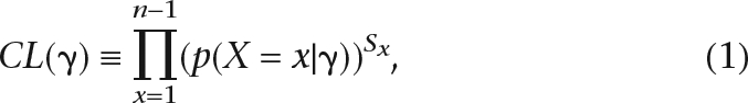where S_x is the number of SNPs of type x, i.e., the number of SNPs with the derived allele segregating at a frequency of x/n in the sample. Error models can be incorporated into the calculation of this likelihood function. Estimates of γ are then obtained by maximizing CL(γ) with respect to γ. This method can be generalized to multiple populations by considering the joint probability of the SNP frequencies in the populations. If the SNPs are in linkage disequilibrium, and therefore not independent, the result of this procedure is not a maximum likelihood estimate. However, this type of estimator can nonetheless be shown to have desirable statistical properties, such as consistency under quite general conditions (Wiuf 2006). In some cases, the composite likelihood estimators are identical to classical estimators. For example, the maximum composite likelihood estimator of θ is identical to Watterson’s (Watterson 1975) estimator of θ, which was originally derived as a method of moments estimator.

The CLEs can be generalized to tiled population genetic data, by summing over all possible (unknown) chromosomal sample sizes in a segment. The marginal sampling distribution for a single SNP from a particular segment can then be calculated as

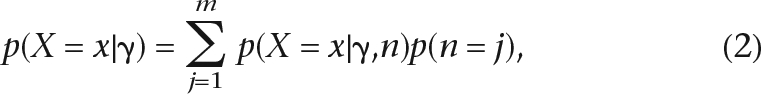where m is the alignment depth (number of reads) for the particular SNP and n is the number of distinct chromosomes (the same chromosome may have been sampled twice). p(n = j), the distribution of the number of distinct chromosomes in a segment, can usually be calculated fairly easily by taking into consideration the procedure used to sample the sequencing reads. In the Methods section, it is described how to calculate p(n = j) if the identity with respect to an individual is known for each sequence. However, similar expressions can also be obtained if this is not known.

The method can also be extended to data from multiple populations by considering the joint frequency spectrum from the populations. For example, for two populations, the data for a single SNP consists of the allelic counts, X₁ and X₂, in the two populations. The likelihood function in a single SNP is then p(X₁ = x₁,X₂ = x₂|γ), and everything follows as before. However, in this study we will treat the data as if it has been sampled from only one population.

The estimator of θ we develop is a modification of Watterson’s (Watterson 1975) classical estimator applicable to the tiled shotgun sequencing data. It assumes an infinite sites model and a constant sequencing error rate. It can be derived as a composite likelihood estimator, but in the Methods section we provide a simpler derivation based on the method of moments. We assume that the alignment can be divided into v segments, where the v − 1 divisions between segments are chosen to fall at the points where a sequencing read starts or ends (Fig. 1). The estimator is then obtained by calculating the expected number of true SNPs and false SNPs due to errors in a segment. By summing over all segments in the alignment, the total expected number of SNPs (including errors) can be calculated, and an estimator can be constructed (see Methods):

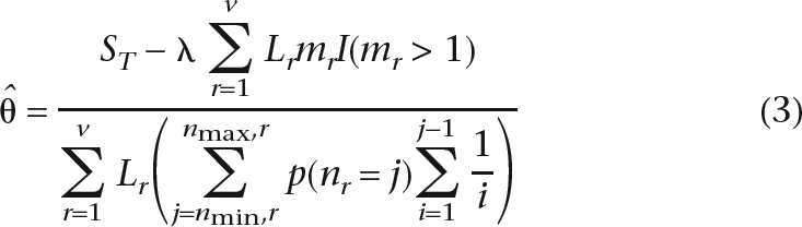where S_T is the total number of segregating sites summed over all segments, and variables subscripted by r are calculated for the rth segment; λ is the error rate per base; L_r, m_r, n_r, n_max,r, n_min,r are the length, the number of reads, the number of distinct chromosomes, and the minimum and the maximum number of distinct chromosomes in segment r.

Figure 1.

Schematic drawing of shotgun reads for one window. The colored bars represent the reads; each color corresponds to a different individual. For our analysis, the window is subdivided into v different segments, so that the sampling depth of reads is invariable within a segment. For example, in segment r_i, we have sampled five reads, corresponding to three individuals, and two individuals have been sampled twice. Therefore, the minimal and maximal number of chromosomes sampled is n_min = 3 and n_max = 5, respectively.

The assumption of errors occurring at a constant and independent rate is not necessarily realistic for DNA sequence data, but deviations from this assumption may not affect the analysis much, as long as the analysis is done on a regional scale and read-by-read variance of the error rate averages out over larger regions. However, it is clearly desirable to develop more accurate error models for particular types of data. Such error models can be incorporated directly into the population genetic analysis by modifying the expression for the expected number of errors in the region.

Genome-wide estimates of nucleotide diversity in humans

For purposes of estimating θ, we will use the original whole-genome shotgun sequences by Celera Genomics (Venter et al. 2001) and the associated SNP-discovery data (see Methods) that contains DNA from seven individuals. The SNPs in conjunction with the mappings of the actual shotgun reads allowed us to obtain genome-wide estimates of nucleotide diversity. We used a window of 100 kb, sliding it by steps of 20 kb. The average sequence coverage within the windows was on average five reads for each segment, which corresponds to approximately two chromosomes. In order to quantify the statistical uncertainty around our estimates, we conducted neutral coalescent simulations under realistic recombination and mutation rates (see Methods). The coefficient of variation in the estimate of θ for 100-kb windows for this simulated data ranged from 0.1 to 0.67 (Supplemental Fig. S1). This indicates that, although the average sample size in number of chromosomes is low, there is useful information regarding in 100-kb windows. On average, we estimate to be 0.00163, a value somewhat higher than is generally cited, and possible reasons for the difference are given below.

The effect of selection on in the human genome

Negative selection (e.g., background selection) and positive selection (e.g., selective sweeps due to hitch-hiking), reduce the average nucleotide diversity at linked neutral sites (Begun and Aquadro 1992; Charlesworth et al. 1993). The number of affected linked sites depends on the recombination rate per site per generation (ρ). Therefore, if either background selection (BS) or hitch-hiking (HH) are common, regions of low recombination are expected to have a lower diversity than regions with high recombination.

Innan and Stephan (2003) suggested a simple method to distinguish between the two types of selection. This method is based on two simplified equations that describe the reduction in neutral diversity θ₀ under a model of BS and HH. In the BS model

if ρ is not extremely low, the reduction in diversity due to background selection is well approximated by e^-u/ρ, where u is the deleterious mutation rate per base per generation. In the HH model:

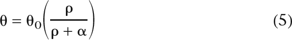the reduction of θ₀ due to selective sweeps depends mainly on ρ and one additional factor α, which is a function of the frequency and strength of selection. We fit each of these models to the data using a simple least squares fit (see Methods). The parameter estimates resulting from this fit are α = 6 × 10⁻¹¹ and θ₀ = 1.67 × 10⁻³ for the HH model; and u = 5 × 10⁻¹¹ and θ₀ = 1.67 × 10⁻³ for the BS model.

When we plot against ρ, there is a clear reduction at very low recombination rates that fits rather well with both the BS- and HH-model (Fig. 2A). However, this reduction in diversity at low recombination rates is incompatible with neutral models, including various demographic scenarios that predict no correlation between recombination and diversity. Therefore, we suggest that selection is indeed important in shaping variability in the human genome.

Figure 2.

Relationship between recombination rate and diversity. Non-overlapping windows were ordered according to recombination rate and sorted into bins of 100 windows. (A) The average /d for the bins was plotted against the average recombination rate as log(ρ), where ρ is the number of recombinants per base per meiosis (red line). For these binned data, we also estimated the parameters for a simple hitchhiking model (HH, cyan line) and a simple background selection model (BS, purple line). /d vs. log(ρ) is also drawn for 100 simulated data sets under the BS-model (black lines). (B) For 100 data sets simulated under the BS-model, we estimated the parameters for the HH- and BS-models. Given these new estimates, we counted how often the BS-model fits better than the HH-model by using the sum of squares and bootstrapping over the bins. In most cases, the BS-model fit consistently better (bootstrap-value closer to 1); but for the real data, the HH-model gave a slightly better fit (cyan arrow).

In 1000 bootstrap samples of the data (see Methods), the HH-model provided, in all but one case, a better fit than the BS-model. We also simulated data under a BS model given the estimated parameter values, and applied the same bootstrapping procedure to each of the simulated data sets (Fig. 2B). In 73 out of 100 simulated cases, the bootstrap support for the BS-model was >0.5, and in all cases, the bootstrap support for the BS-model was higher than in the real data. These results suggest that the HH-model provides a better fit to the data than the BS-model, and that the BS-model cannot fully explain the pattern observed in the data. However, we emphasize that the BS-model used here is very simple, and it makes a number of assumptions in addition to the absence of selective sweeps. Our results should, therefore, not be taken as proof of absence of background selection in humans, but may suggest that the effect of selection in the genome cannot be explained by the simple BS-model alone and that selective sweeps might be the more dominant force that shapes genetic diversity across the human genome.

Identifying outliers

In order to identify candidate regions for recent selective sweeps and balancing selection, we conducted coalescent simulations in a sliding window along the genome, taking the observed distribution of sequence reads, local mutation rate estimated from human–chimpanzee divergence (d), and local recombination rate into account (see Methods). Furthermore, we did half of the simulations under the best-fitting background selection model (see above). The expected value of θ, given these factors, is denoted by θ_E. The 324 and 80 regions in the genome had smaller and larger values of , respectively, than any of the 2000 simulations for the region. The 10 regions with the lowest values of /θ_E are given in Table 1 and the 10 regions with the highest values of /θ_E are summarized in Supplemental Table S2. Regions that have recently experienced a selective sweep should be marked by a low /θ_E. However, as the expected value of θ_E will be calculated based on d, an increased d could have a similar effect. Similarly, an increased /θ_E may be indicative of balancing selection (Kreitman and Hudson 1991), but might also be caused by misassemblies of the human shotgun reads, or reduced levels divergence. We compare our results with other genome-wide scans for selection in Table 2.

Table 1.

Position of the 10 regions with the lowest /θ_E within the human genome version hg16

The closest gene to the 100-kb window with the lowest /θ_E is reported if within 200 kb of the reported candidate region. The description was mostly adapted from the Known Gene annotation of the genome browser (Hsu et al. 2006).

^aGene does not overlap with reported region, but is within 200 kb.

Table 2.

Number of nonoverlapping 100-kb windows that overlap with selected regions, as identified in other studies

Here, windows with /θ_E lower or higher than 95% of the simulated data, respectively, were compared. Significance of the overlap between high and low /θ_E windows and other studies was assessed using Fisher’s exact test.

^aData from Supplementary Protocols 1–3 were merged to form unique genomic regions.

^bData from Table 1 and Supplemental Table S1.

^cData from Supplemental Tables S2–S9 were merged to form unique genomic regions.

^dOverlap of data is based on mappings the RefSeq and Known Gene tables of the UCSC genome browser.

Regions with high /θ_E are candidates for balancing selection or they might contain more slightly deleterious variants, i.e., substitutions that can segregate within a population, but are unlikely to become fixed. In protein-coding regions, both possibilities result in an excess of nonsynonymous polymorphisms, as can be detected in a McDonald-Kreitman test. Indeed, if we match the high /θ_E regions to genes identified in Bustamante et al. (2005) to be under negative selection, we find them to be significantly enriched (Table 2). Furthermore, the HLA-cluster on chromosome 6 contains five regions with highly elevated /θ_E (Supplemental Fig. S4), of which one is the second highest overall (Supplemental Table S2). This is encouraging because the HLA-region has previously been shown to evolve under balancing selection (Klitz et al. 1986; Erlich and Gyllensten 1991; Begovich et al. 1992; Hughes et al. 1993). Furthermore, we also find that large clusters of olfactory receptors (as annotated in Aloni et al. 2006 and with more than three human genes), exhibit unusually high values of /θ_E (Table 2). The largest cluster with 103 genes in humans is located on chromosome 11. This region encompasses ∼1 Mb and contains five /θ_E peaks (Supplemental Fig. S5). Another chromosome 11 olfactory receptor cluster has previously been shown to be under positive selection (Clark et al. 2003; Gilad et al. 2003; Nielsen et al. 2005). Further indication that high regions may also have experienced selective sweeps is that they show a significant overlap with the regions of recently selected genes as identified by Tang et al. (2007).

A third possible explanation for elevated /θ_E are copy number polymorphisms where a copy is gained. Indeed, the region with the highest value of /θ_E is surrounded by common copy number polymorphisms (CNPs). The actual peak in /θ_E does not lie within a known copy number gain, suggesting that the increased value of /θ_E has not been inflated by a gain in copy number in one or more individuals compared to the assembly. However, CNPs may affect alignments, thereby inflating .

Characterizing extreme /θ_E regions

We summarize the results for gene-specific analyses of regions with elevated or reduced values of /θ_E by dividing genes into different GO categories (Ashburner et al. 2000). RefSeq genes were associated with the nonoverlapping windows, and if a window contained multiple genes with the same GO category, this GO category was only counted once for this window. Thus, we avoid GO categories from becoming significant, just because of one cluster of genes. For example, unlike other studies, we do not find the GO categories related to olfaction to be significant, although individual OR clusters show clear signals. We find that all three ontologies—biological process, cellular component, and molecular function—show a significant enrichment of outlier regions in certain GO categories (Supplemental Table S3). We show a comprehensive summary of the results for what we consider the most informative category, biological process, in Supplemental Table S5.

Regions with reduced /θ_E contain an enrichment of categories traditionally associated with selective sweeps and positive selection (Chimpanzee Sequencing and Analysis Consortium 2005; Nielsen et al. 2005; Gibbs et al. 2007), including the following immune response related categories: regulation of B cell activation, B cell differentiation, and leukocyte chemotaxis (Supplemental Table S5). Other immune-related categories and categories involved in apoptosis are not among the most significant categories (Supplemental Table S4). One explanation for this is that these categories are also more likely to have experienced balancing selection, and hence also have an elevated /θ_E. This is true for several apoptosis related groups (Supplemental Table S6).

The region in the genome with the lowest value of /θ_E is the cystatin cluster on chromosome 20 (Table 1). The cystatins in this cluster are potent inhibitors of cysteine proteases, especially cathepsin B. The cystatins in the middle of the /θ_E valley belong to the S-cystatins (Supplemental Fig. S6), which are abundant in saliva, but occur also in other body fluids such as tears. Presumably, they have a protective function. However, this does not appear to fully explain their abundance in saliva (Dickinson 2002).

The region with the second lowest value of /θ has only one gene in its proximity, and that is the ephrin receptor A6 (Fig. 3). Ephrin receptors are a large family of protein tyrosine kinase receptors. They play an important role in axon guidance, especially during brain development (Yun et al. 2003). Furthermore, ephrin receptors are involved in vasculogenesis and angiogenesis (Cheng et al. 2002), and EPHA6 has been shown to be a regulator of vascularization of genital tubercles (Shaut et al. 2007). The protein sequence of EPHA6 is highly conserved from human to chicken, and most of the variability occurs in the ligand-binding domain. However, this domain is also completely conserved between humans and chimpanzees, suggesting that the most likely target of selection was a regulatory change.

Figure 3.

The area around the second lowest value of /θ_E on chromosome 3. Vertical bars represent the values for a 100-kb window positioned at their midpoint. (A) Plotted is /θ_E, whereas the expected value is either under a neutral or a background selection model, whatever was more conservative. The colors of the bars indicate whether /θ_E lie outside of a 95%, 96%, etc., confidence interval obtained through simulations. (B) Pink triangles mark recombination hotspots; blue lines correspond to genes from the RefSeq gene track of the UCSC genome browser. The closest gene is EPHA6. (C–E) The values for , human–chimpanzee divergence, and the recombination rate in cM/Mb are plotted.

We think that these two loci might be interesting cases of recent selection that are worthwhile to study in more depth.

Subcentromeric regions

Subcentromeric regions generally have very low recombination rates (Yu et al. 2001; Kong et al. 2002). Consequently, centromeres may have a reduced level of diversity under both a model of background selection and of selective sweeps. Additionally, centromeric repeats are thought to be prone to meiotic drive acting during female meiosis (for review, see Henikoff et al. 2001). Subcentromeric regions may, therefore, be affected by selective sweeps more frequently than other genomic regions. A previous scan for selective sweeps in the human genome (Williamson et al. 2007) found increased evidence for selective sweeps around centromeric regions.

We define windows as centromeric if they overlap with the chromosomal band labeled as centromeric in the UCSC genome browser (http://genome.ucsc.edu). As expected, these windows are associated with extremely low recombination rates (Fig. 4A). Furthermore, appears to be reduced, while human–chimpanzee divergence is increased relative to intrachromosomal regions (Fig. 4B,C). Taking background selection and mutation rates into account in the calculation of θ_E (Fig. 4D), we find that in subcentromeric regions is still significantly lower than expected (MWU-test: n = 159, P = 1.5 × 10⁻⁶). This result strongly suggests that selective sweeps are, in fact, more common in centromeric regions.

Figure 4.

Centromeres (cen) and Telomeres (tel) behave differently from intrachromosomal (ic) regions in their recombination rates (A), diversity (B), human–chimpanzee divergence (C), and hence, also in the predicted value θ_E (D). However, for centromeres and telomeres is smaller than θ_E.

Such a picture could also emerge if the number of chromosomes (n) was overestimated due to assembly errors. As the number of reads (m) in the alignment is indeed elevated for the centromeres (Fig. 4C), this is a possible explanation. Therefore, we excluded all centromeric regions with m among the 25% most extreme values of m genome-wide. In this analysis still remains significantly lower than expected (MWU-test: n = 112, P = 0.009). Therefore, we believe that the reduction in centromeric diversity is indeed due to positive selection, consistent with the theory of a centromeric meiotic drive.

Subtelomeric regions

One of the unexplained results from the analysis of the chimpanzee genome was the observation of increased divergence in subtelomeric regions (Fig. 4C; Chimpanzee Sequencing and Analysis Consortium 2005). Another hallmark of these regions is a relatively high recombination rate (Fig. 4A; Kong et al. 2002). One possible explanation for the high levels of divergence is the mutagenic effect of recombination (Lercher and Hurst 2002; Hellmann et al. 2003), identified as a positive correlation between divergence and recombination. This pattern appears to be mediated at least in part by the hypermutability of CpGs and the elevation of recombination in regions of high GC content. Subtelomeric regions appear to fit this same pattern, with elevated divergence and recombination rates. Dreszer et al. (2007) found evidence that biased gene conversion has major contributions to elevated substitution rates in conjunction with high GC content and recombination rates. However, the effect of recombination cannot be the only reason, as other regions of the genome with similar recombination rates have lower levels of divergence than the subtelomeric regions (MWU-test, telomeric vs. subsample intrachromosomal: n = 1175; P(d) < 10⁻¹⁵; P(ρ) = 0.34, Supplemental Fig. S3).

As was the case for subcentromeric regions, subtelomeric regions also show a decrease in /θ_E (MWU-test: n = 1175, P < 10⁻¹⁵), possibly suggesting increased levels of selective sweeps in telomeric regions. Unlike centromeres, telomeric repeats show no evidence of meiotic drive. However, telomeres are enriched for segmental duplications (for review, see Cheng et al. 2005; Riethman et al. 2005), and hence, one could speculate that subtelomeric regions are hubs for neofunctionalization of duplicate genes and, therefore, more variants are fixed due to positive selection.

Discussion

Our average estimate of = 0.00163, is higher than in other studies. Halushka et al. (1999) reported estimates of θ based on numbers of segregating sites for silent substitutions of 0.0015 and for introns of 0.00105. The estimates from the resequenced data in the Seattle SNP database (http://pga.gs.washington.edu/summary_stats.html; Akey et al. 2004), based on the average number of pairwise differences is 0.00085. One explanation for the difference between the results by Akey et al. (2004) and our results is that the Seattle SNPs data set only includes genic regions. However, our estimate is also higher than the estimate from 50 intergenic regions (Voight et al. 2005). A slight difference in the estimates is expected, because our estimator based on the number of segregating sites will give higher estimates than the estimator based on pairwise differences in the presence of a negative Tajima’s D value, as observed for the Seattle data and at least one population of the Voight data. Further, Voight et al. (2005) report only diversity for the populations separately, but not the overall diversity. Finally, as pointed out in Johnson and Slatkin (2006), estimates of θ may be biased when quality values have been used to call SNPs. As our data have been subject to an initial quality screening, it is likely that our data are also affected by this bias. However, in the absence of regional differences in the use of protocols to call SNPs, none of our conclusions should be affected by this bias.

Furthermore, our estimate of diversity was made without correction for demographic influences. In part, this is because the sample for the Celera Genomics study included an overdispersed sampling of humans from the major geographic groups. Therefore, we want to stress that the P-values and confidence intervals that we obtain through the simulations are only exact if the assumptions of our simulations were right. If we overestimate, or the individuals that we analyzed did not come from a Wright-Fisher population but from a population with a more complex demography, we may, for some demographic models, underestimate the variance of .

We examined the overlap between regions with low values of /θ_E and regions identified in other genome-wide screens for positive selection. Voight et al. (2006) conducted a genome-wide screen for selective sweeps based on haplotype structure. This method has maximal power to detect ongoing selective sweeps, while the reduction in diversity that we measure is strongest after a sweep has just finished. Therefore, the lack of overlap in candidate regions identified by the two studies is not surprising (Table 2). Next, we looked for overlap between our data and the data by Williamson et al. (2007). Their test statistic is based on the frequency spectrum at variable sites and, hence, their power is also best for finished sweeps. However, since the statistic only looks at variable sites, the power of this test for regions of very low diversity will also be lower than in our test. This might explain why we find so little overlap in candidate regions. Another possible cause is that our confidence intervals are widest for regions of low recombination. Therefore, the average recombination rate of our candidate regions is 1.87 cM/Mb, while the two LD studies show an opposite trend (median recombination rates: 0.76 and 1.2 cM/Mb). On the other hand, there is good overlap between our candidate regions and regions identified in a recent study contrasting patterns of LD among different populations to detect nearly complete selective sweeps (Tang et al. 2007).

Further, we find a significant overlap with the study by Bustamante et al. (2005) and the clusters of positively selected genes as identified by the Chimpanzee Sequencing and Analysis Consortium (2005) (Table 2). Both studies use the ratio of nonsynonymous to synonymous mutations in human–chimpanzee alignments to detect selection within protein-coding genes. Bustamante et al. additionally used ratios of nonsynonymous to synonymous human diversity in an extension of the McDonald-Kreitman test (McDonald and Kreitman 1991). If no selection were acting in the genome, we would not expect a correlation between diversity to divergence ratios and ratios of nonsynonymous to synonymous mutations. The strong correspondence between the studies, therefore, helps solidify the argument that extreme values of /θ_E, in fact, do provide evidence for positive selection.

A number of factors can affect the analyses presented in this study. The methods used for identifying SNPs and accommodating sequencing, assembly, and alignment errors may affect local estimates of genetic diversity. Future studies may incorporate more specific and detailed modeling of errors based on experimental evidence and genotype confidence scores. We also notice that we used a very simple standard population genetic model, assuming constant population sizes and no population structure. Finally, the sample size is very low (seven individuals from diverse racial groups) with one individual contributing a large proportion of the reads analyzed. However, the main conclusions of the study stand and are unlikely to be influenced by this: (1) tiled population genetic data can easily be dealt with in population genetic analyses using appropriately modified composite likelihood methods, (2) the human genome shows a reduction in variability in regions of low recombination that cannot be explained by possible mutagenic effects of recombination, (3) both telomeres and centromeres show a decrease in the levels of diversity compared with the expectation given between-species divergence and recombination rate, (4) outlier analyses of variability identify a number of candidate genes for both balancing and directional selection including HLA and olfactory receptor clusters. However, our ability to reliably identify outlier regions may be challenged if there is an undetected regional variation in the error rate.

While even this relatively simplistic approach to demography and sequence errors will see immediate application, an exciting challenge in future studies is to incorporate inference procedures for more elaborate and realistic models. This can be achieved using the composite likelihood framework outlined in this study.

Methods

SNPs from shotgun data

This procedure was described in dbSNP under http://www.ncbi.nlm.nih.gov/projects/SNP/snp_viewTable.cgi?method_id=2929. Briefly, potential nucleotide variants from the WGA2 alignment were identified using only the Celera reads. Potential nucleotide variants need to pass the sequence quality value (QV), neighbor quality value (NQV), and the heterozygosity check. The default QV value is >23 for the polymorphic base and >21 for the minimal neighbor QV (4 bp). For the deep covered minor alleles, the QV threshold is adjusted lower. Every supported minor allele will decrease the threshold, but the minimal QV cutoff is not below 16. During the heterozygosity check, sequences containing more than two alleles per individual were filtered out.

The locations of all reads were mapped relative to the assembly. We then divided the shotgun assembly and associated SNPs into segments according to shotgun read ends (Fig. 1). In order to be able to use annotations based on the public human genome version (hg16), we placed the segments on this assembly.

Error rate λ

Based on Altshuler et al. (2000), we assumed that the error rate λ = 1/35,000, which most likely corresponds to an upper bound. If we assume that the error rate is approximately constant, the actual value of λ influences θ linearly. Further, the number of expected errors is on average 20-fold lower than our SNP counts; hence, the relative magnitude of θ should be robust with respect to assumptions about λ.

Human–chimpanzee divergence

We downloaded the axt—alignments between the human genome hg16 and the chimpanzee genome panTro2 (http://hgdownload.cse.ucsc.edu/goldenPath/hg16/vsPanTro1/axtRBestNet/). For each window, we counted the number of bases that differed and divided them by the number of bases that could be compared.

Recombination rates

We downloaded genetic and physical distances from http://www.stats.ox.ac.uk/mathgen/Recombination.html and calculated the recombination rates as slopes from regressing genetic on physical distance for windows of 500 kb centered on a given 100-kb window. Here, estimates of recombination rate are based on patterns of LD; therefore, there may be concerns that the estimates of recombination rates depend on SNP density. However, SNP density mainly influences estimates of variation in recombination rate (e.g., inferences of recombination hotspots) and not so much the average rate over large distances as examined here. Also, the difference in recombination rate estimates between pedigree map (Kong et al. 2002) and the LD map does not vary systematically with (Supplemental Fig. S2). Hence, it seems like an acceptable approximation to use the LD map for this purpose.

Estimating θ

The estimator of θ we develop is a modification of Watterson’s (Watterson 1975) classical estimator applicable to the tiled shotgun sequencing data. It can be derived as a composite likelihood estimator, but we will provide the simpler derivation using a method of moments estimator. To this end, we divide the genome into v segments, where the v − 1 divisions between segments are chosen to fall at the points where a fragment starts or ends (Fig. 1). The number of sequences sampled is, therefore, constant among all nucleotide positions within a segment. For example, in an alignment of two sequences, which overlap each other, there can be three such segments. To write down simple expressions for p(n = j) for a particular segment, we need to introduce some additional notation to distinguish between the number of reads sampled, the number of distinct chromosomes sampled, the number of reads from an individual, the number of distinct chromosomes from an individual, etc. Let x represent one segment. We can think of x as a set of equivalence classes, x₁, x₂, . . . , each representing sequences sampled from the same (diploid) individual. Let |x| be the number of equivalence classes (individuals) in x and |x_i| be the number of elements (sequencing reads) in equivalence class i, i.e., |x_i| is the number of sequencing reads from individual i, and |x| is the number of individuals. We assume throughout that the reads are labeled with regard to which individual they come from. Also, n and n_min = |x| represent the number of distinct chromosomes (although possibly identical at the nucleotide level) and minimum number of distinct chromosomes, respectively, in the segment. The chance that an individual with |x_i| ≥ 1 reads is represented by one or two chromosomes in the alignment is 0.5^|x_i|−1 and 1 − 0.5^|x_i|−1, respectively. Then, the probability of n = j is given by summing over all the possible ways the number of distinct reads among individuals represented in the alignment could sum up to j:

where I(. . .) is an indicator function. Even for large samples, this expression can be calculated fast using a dynamic programming algorithm.

For n chromosomes, in the absence of sequencing errors and assuming an infinitely many sites model (Watterson 1975), the expected number of segregating sites in a segment of length L is (Watterson 1975) L(θ∑(1/i)). The expected number in a tiled alignment is then obtained similarly by summing over all possible values of n. The expected number or false SNPs introduced by sequencing errors is LλmI(m > 1) + O(λ²) as λ → 0, where λ is the sequencing error rate per nucleotide and m is the total number of reads in the segment. Assuming that the error rate is low enough that two sequencing errors in the same site can be ignored, the expected number of segregating sites for tiled data in an alignment segment is:

Note that this assumes that errors occur uniformly and independently of neighboring nucleotides. From this, an unbiased estimator of similar to the Watterson (1975) estimator can be obtained by rearranging (Equation 2) and summing over alignment segments (Equation 3).

Confidence intervals for

The variance in cannot be obtained analytically in the presence of recombination, even for complete data that has not been obtained by shotgun sequencing. Only in the presence of no recombination or full recombination, i.e., no linkage disequilibrium among SNPs, can formulas for the variance be obtained. Such formulas can also be derived for tiled shotgun data, but are not of much practical use, as linkage disequilibrium is indeed widely observed in most data. Our approach for the estimation of confidence intervals is, therefore, based on simulating data, taking into account variation in local recombination rates, sequencing errors, and the number of reads sampled for any particular genomic segment. To this end, we used the program ms to do coalescent simulations (Hudson 2002) under the standard neutral model and a simple background selection model, which will be described below. After we obtain the sample sequences from the coalescent simulations, we sample “reads” from those sequences in exactly the same way as they were obtained from the Celera data, and then calculate as described.

Parameter estimation under selection models

In order to estimate the selection parameters α and u, we need to correct for variation in θ₀ due to mutation rate variation. To this end, we scaled θ₀ using a scalar c_i for window i based on estimates of chimpanzee–human divergence as proxies for mutation rate variation. Estimates of ρ for each window were calculated from the Myers-map (Myers et al. 2005). Because these simple models assume that the strength and frequency of positive and negative selection is constant across the genome, we decided to reduce the noise by binning the data according to recombination rates. We sorted nonoverlapping windows according to their recombination rate into bins of 100. Then, we fitted the models of selection described in Equations 4 and 5 to the binned data, thus obtaining estimates of θ₀, α, and u.

The model was fitted using the Nelder-Mead Simplex algorithm as implemented in the Gnu Scientific library (http://www.gnu.org/software/gsl/) using least squares as a test-statistic. We also attempted to fit the model to unbinned data; however, the model fit, as assessed by a simple sum of squares, was always inferior to that obtained with summarized data. We also tried a more complicated model of background selection that could also accommodate variation in recombination rates across the flanking regions of each window. Again, as for the simple model and the unbinned data, the more complicated model failed to fit the data better.

In order to compare the fit of the BS and HH models, we generated 1000 bootstrap samples over bins and counted how often the least squares statistics was better for either the BS or the HH-model.

Simulations under the background selection and a neutral model

We used the program ms for all coalescent simulations (Hudson 2002). For coalescent simulations under a background selection model, we reduced the effective population size by e^–u/ρ, where u is the deleterious mutation rate per generation per base pair and ρ is the number of crossovers per generation per base pair. For each window i, we simulated for θ_E = θ₀e^−u/ρ_ic_i, where θ₀ is the average diversity. c_i is a scalar allowing variation in the mutation rate, calculated as c_i = d_i/d, whereas d_i is the human–chimpanzee divergence of window i and d is the mean divergence.

Thus, we simulated 14 chromosomes. We then subsampled segments from these chromosomes, corresponding to the segments obtained from the Celera shotgun reads. The probability that both chromosomes from an individual were sampled was taken as p = 1 − 0.5^x_rj−1, where x_rj is the number of reads from individual j in segment r.

To simulate sequencing errors, we added S_e errors drawn from a Poisson distribution with mean λ∑L_rm_rI(m_r > 1), where L_r is the length of the segment r in bp, m is the number of reads in segment r, and I is and indicator function.

Outlier analysis

In order to identify candidate regions for recent selective sweeps and balancing selection, we conducted 200 coalescent simulations (100 under the standard neutral and 100 under a BS-model) for each 100-kb window, sliding by 20 kb, taking the observed distribution of sequence reads in each window into account, and using a window-specific value of θ to drive the simulations. We identified all windows with observed values of falling outside the distributions of in the simulated data under both neutrality and background selection. Those windows were merged with all adjacent windows where fell among the 5% most extreme values on either side in the simulated data. For the resulting 1046 regions with elevated values and 589 regions with reduced values of we conducted another 2000 simulations to get a more precise estimate of the P-value (Supplemental Table S1).

Gene Ontology analysis

All locuslink genes overlapping with the 1046 high or 589 low regions as well as all nonoverlapping 100-kb windows outside of these regions were identified. The locuslink identifiers were then used in BioMart (Kasprzyk et al. 2004) to associate locuslink identifiers with Gene Ontology groups (GO) (Ashburner et al. 2000). We only took reviewed annotations into account, i.e., we disregarded annotations with evidence code IEA and ND. The Gene Ontology version from May 2007 was used. For each region/window only a nonredundant set of GO-identifiers was kept. To identify GO-groups with over-representations of either high /θ_E or low /θ_E regions, we used the program FUNC (Prufer et al. 2007). More specifically, we used the hypergeometric test, requiring a minimum of 10 windows associated with a given node. After obtaining the general statistics for each ontology, we made use of the refinement option in FUNC that keeps only the most specific, significant categories; higher categories that are solely significant because of genes from a significant subordinate category are removed.

References

- Adams A.M., Hudson R.R. Maximum-likelihood estimation of demographic parameters using the frequency spectrum of unlinked single-nucleotide polymorphisms. Genetics. 2004;168:1699–1712. doi: 10.1534/genetics.104.030171. [DOI] [PMC free article] [PubMed] [Google Scholar]
- Akey J.M., Eberle M.A., Rieder M.J., Carlson C.S., Shriver M.D., Nickerson D.A., Kruglyak L. Population history and natural selection shape patterns of genetic variation in 132 genes. PLoS Biol. 2004;2:e286. doi: 10.1371/journal.pbio.0020286. [DOI] [PMC free article] [PubMed] [Google Scholar]
- Aloni R., Olender T., Lancet D. Ancient genomic architecture for mammalian olfactory receptor clusters. Genome Biol. 2006;7:R88. doi: 10.1186/gb-2006-7-10-r88. [DOI] [PMC free article] [PubMed] [Google Scholar]
- Altshuler D., Pollara V.J., Cowles C.R., Van Etten W.J., Baldwin J., Linton L., Lander E.S. An SNP map of the human genome generated by reduced representation shotgun sequencing. Nature. 2000;407:513–516. doi: 10.1038/35035083. [DOI] [PubMed] [Google Scholar]
- Andolfatto P. Adaptive evolution of non-coding DNA in Drosophila. Nature. 2005;437:1149–1152. doi: 10.1038/nature04107. [DOI] [PubMed] [Google Scholar]
- Andolfatto P., Przeworski M. Regions of lower crossing over harbor more rare variants in African populations of Drosophila melanogaster. Genetics. 2001;158:657–665. doi: 10.1093/genetics/158.2.657. [DOI] [PMC free article] [PubMed] [Google Scholar]
- Ashburner M., Ball C.A., Blake J.A., Botstein D., Butler H., Cherry J.M., Davis A.P., Dolinski K., Dwight S.S., Eppig J.T., et al. Gene Ontology: Tool for the unification of biology. The Gene Ontology Consortium. Nat. Genet. 2000;25:25–29. doi: 10.1038/75556. [DOI] [PMC free article] [PubMed] [Google Scholar]
- Begovich A.B., McClure G.R., Suraj V.C., Helmuth R.C., Fildes N., Bugawan T.L., Erlich H.A., Klitz W. Polymorphism, recombination, and linkage disequilibrium within the HLA class II region. J. Immunol. 1992;148:249–258. [PubMed] [Google Scholar]
- Begun D.J., Aquadro C.F. Levels of naturally occurring DNA polymorphism correlate with recombination rates in D. melanogaster. Nature. 1992;356:519–520. doi: 10.1038/356519a0. [DOI] [PubMed] [Google Scholar]
- Bentley D.R. Whole-genome re-sequencing. Curr. Opin. Genet. Dev. 2006;16:545–552. doi: 10.1016/j.gde.2006.10.009. [DOI] [PubMed] [Google Scholar]
- Bustamante C.D., Fledel-Alon A., Williamson S., Nielsen R., Hubisz M.T., Glanowski S., Tanenbaum D.M., White T.J., Sninsky J.J., Hernandez R.D., et al. Natural selection on protein-coding genes in the human genome. Nature. 2005;437:1153–1157. doi: 10.1038/nature04240. [DOI] [PubMed] [Google Scholar]
- Charlesworth B., Morgan M.T., Charlesworth D. The effect of deleterious mutations on neutral molecular variation. Genetics. 1993;134:1289–1303. doi: 10.1093/genetics/134.4.1289. [DOI] [PMC free article] [PubMed] [Google Scholar]
- Cheng N., Brantley D.M., Chen J. The ephrins and Eph receptors in angiogenesis. Cytokine Growth Factor Rev. 2002;13:75–85. doi: 10.1016/s1359-6101(01)00031-4. [DOI] [PubMed] [Google Scholar]
- Cheng Z., Ventura M., She X., Khaitovich P., Graves T., Osoegawa K., Church D., DeJong P., Wilson R.K., Paabo S., et al. A genome-wide comparison of recent chimpanzee and human segmental duplications. Nature. 2005;437:88–93. doi: 10.1038/nature04000. [DOI] [PubMed] [Google Scholar]
- Chimpanzee Sequencing and Analysis Consortium Initial sequence of the chimpanzee genome and comparison with the human genome. Nature. 2005;437:69–87. doi: 10.1038/nature04072. [DOI] [PubMed] [Google Scholar]
- Clark A.G., Glanowski S., Nielsen R., Thomas P.D., Kejariwal A., Todd M.A., Tanenbaum D.M., Civello D., Lu F., Murphy B., et al. Inferring nonneutral evolution from human-chimp-mouse orthologous gene trios. Science. 2003;302:1960–1963. doi: 10.1126/science.1088821. [DOI] [PubMed] [Google Scholar]
- Dickinson D.P. Salivary (SD-type) cystatins: Over one billion years in the making—But to what purpose? Crit. Rev. Oral Biol. Med. 2002;13:485–508. doi: 10.1177/154411130201300606. [DOI] [PubMed] [Google Scholar]
- Donnelly P., Tavare S. Coalescents and genealogical structure under neutrality. Annu. Rev. Genet. 1995;29:401–421. doi: 10.1146/annurev.ge.29.120195.002153. [DOI] [PubMed] [Google Scholar]
- Dreszer T.R., Wall G.D., Haussler D., Pollard K.S. Biased clustered substitutions in the human genome: The footprints of male-driven biased gene conversion. Genome Res. 2007;17:1420–1430. doi: 10.1101/gr.6395807. [DOI] [PMC free article] [PubMed] [Google Scholar]
- Erlich H.A., Gyllensten U.B. The evolution of allelic diversity at the primate major histocompatibility complex class II loci. Hum. Immunol. 1991;30:110–118. doi: 10.1016/0198-8859(91)90079-o. [DOI] [PubMed] [Google Scholar]
- Gibbs R.A., Rogers J., Katze M.G., Bumgarner R., Weinstock G.M., Mardis E.R., Remington K.A., Strausberg R.L., Venter J.C., Wilson R.K., et al. Evolutionary and biomedical insights from the rhesus macaque genome. Science. 2007;316:222–234. doi: 10.1126/science.1139247. [DOI] [PubMed] [Google Scholar]
- Gilad Y., Bustamante C.D., Lancet D., Paabo S. Natural selection on the olfactory receptor gene family in humans and chimpanzees. Am. J. Hum. Genet. 2003;73:489–501. doi: 10.1086/378132. [DOI] [PMC free article] [PubMed] [Google Scholar]
- Halushka M.K., Fan J.B., Bentley K., Hsie L., Shen N., Weder A., Cooper R., Lipshutz R., Chakravarti A. Patterns of single-nucleotide polymorphisms in candidate genes for blood-pressure homeostasis. Nat. Genet. 1999;22:239–247. doi: 10.1038/10297. [DOI] [PubMed] [Google Scholar]
- Hellmann I., Ebersberger I., Ptak S.E., Paabo S., Przeworski M. A neutral explanation for the correlation of diversity with recombination rates in humans. Am. J. Hum. Genet. 2003;72:1527–1535. doi: 10.1086/375657. [DOI] [PMC free article] [PubMed] [Google Scholar]
- Hellmann I., Prufer K., Ji H., Zody M.C., Paabo S., Ptak S.E. Why do human diversity levels vary at a megabase scale? Genome Res. 2005;15:1222–1231. doi: 10.1101/gr.3461105. [DOI] [PMC free article] [PubMed] [Google Scholar]
- Henikoff S., Ahmad K., Malik H.S. The centromere paradox: Stable inheritance with rapidly evolving DNA. Science. 2001;293:1098–1102. doi: 10.1126/science.1062939. [DOI] [PubMed] [Google Scholar]
- Hsu F., Kent W.J., Clawson H., Kuhn R.M., Diekhans M., Haussler D. The UCSC Known Genes. Bioinformatics. 2006;22:1036–1046. doi: 10.1093/bioinformatics/btl048. [DOI] [PubMed] [Google Scholar]
- Hudson R.R. Two-locus sampling distributions and their application. Genetics. 2001;159:1805–1817. doi: 10.1093/genetics/159.4.1805. [DOI] [PMC free article] [PubMed] [Google Scholar]
- Hudson R.R. Generating samples under a Wright-Fisher neutral model of genetic variation. Bioinformatics. 2002;18:337–338. doi: 10.1093/bioinformatics/18.2.337. [DOI] [PubMed] [Google Scholar]
- Hudson R.R., Kreitman M., Aguade M. A test of neutral molecular evolution based on nucleotide data. Genetics. 1987;116:153–159. doi: 10.1093/genetics/116.1.153. [DOI] [PMC free article] [PubMed] [Google Scholar]
- Hughes A.L., Hughes M.K., Watkins D.I. Contrasting roles of interallelic recombination at the HLA-A and HLA-B loci. Genetics. 1993;133:669–680. doi: 10.1093/genetics/133.3.669. [DOI] [PMC free article] [PubMed] [Google Scholar]
- Innan H., Stephan W. Distinguishing the hitchhiking and background selection models. Genetics. 2003;165:2307–2312. doi: 10.1093/genetics/165.4.2307. [DOI] [PMC free article] [PubMed] [Google Scholar]
- Johnson P.L., Slatkin M. Inference of population genetic parameters in metagenomics: A clean look at messy data. Genome Res. 2006;16:1320–1327. doi: 10.1101/gr.5431206. [DOI] [PMC free article] [PubMed] [Google Scholar]
- Kasprzyk A., Keefe D., Smedley D., London D., Spooner W., Melsopp C., Hammond M., Rocca-Serra P., Cox T., Birney E. EnsMart: A generic system for fast and flexible access to biological data. Genome Res. 2004;14:160–169. doi: 10.1101/gr.1645104. [DOI] [PMC free article] [PubMed] [Google Scholar]
- Klitz W., Thomson G., Baur M.P. Contrasting evolutionary histories among tightly linked HLA loci. Am. J. Hum. Genet. 1986;39:340–349. [PMC free article] [PubMed] [Google Scholar]
- Kong A., Gudbjartsson D.F., Sainz J., Jonsdottir G.M., Gudjonsson S.A., Richardsson B., Sigurdardottir S., Barnard J., Hallbeck B., Masson G., et al. A high-resolution recombination map of the human genome. Nat. Genet. 2002;31:241–247. doi: 10.1038/ng917. [DOI] [PubMed] [Google Scholar]
- Kreitman M., Hudson R.R. Inferring the evolutionary histories of the Adh and Adh-dup loci in Drosophila melanogaster from patterns of polymorphism and divergence. Genetics. 1991;127:565–582. doi: 10.1093/genetics/127.3.565. [DOI] [PMC free article] [PubMed] [Google Scholar]
- Lercher M.J., Hurst L.D. Human SNP variability and mutation rate are higher in regions of high recombination. Trends Genet. 2002;18:337–340. doi: 10.1016/s0168-9525(02)02669-0. [DOI] [PubMed] [Google Scholar]
- Margulies M., Egholm M., Altman W.E., Attiya S., Bader J.S., Bemben L.A., Berka J., Braverman M.S., Chen Z., Chen Y.J., et al. Genome sequencing in microfabricated high-density picolitre reactors. Nature. 2005;437:376–380. doi: 10.1038/nature03959. [DOI] [PMC free article] [PubMed] [Google Scholar]
- McDonald J.H., Kreitman M. Adaptive protein evolution at the Adh locus in Drosophila. Nature. 1991;351:652–654. doi: 10.1038/351652a0. [DOI] [PubMed] [Google Scholar]
- McVean G.A. A genealogical interpretation of linkage disequilibrium. Genetics. 2002;162:987–991. doi: 10.1093/genetics/162.2.987. [DOI] [PMC free article] [PubMed] [Google Scholar]
- Myers S., Bottolo L., Freeman C., McVean G., Donnelly P. A fine-scale map of recombination rates and hotspots across the human genome. Science. 2005;310:321–324. doi: 10.1126/science.1117196. [DOI] [PubMed] [Google Scholar]
- Nielsen R. Estimation of population parameters and recombination rates from single nucleotide polymorphisms. Genetics. 2000;154:931–942. doi: 10.1093/genetics/154.2.931. [DOI] [PMC free article] [PubMed] [Google Scholar]
- Nielsen R., Bustamante C., Clark A.G., Glanowski S., Sackton T.B., Hubisz M.J., Fledel-Alon A., Tanenbaum D.M., Civello D., White T.J., et al. A scan for positively selected genes in the genomes of humans and chimpanzees. PLoS Biol. 2005;3:e170. doi: 10.1371/journal.pbio.0030170. [DOI] [PMC free article] [PubMed] [Google Scholar]
- Polanski A., Kimmel M. New explicit expressions for relative frequencies of single-nucleotide polymorphisms with application to statistical inference on population growth. Genetics. 2003;165:427–436. doi: 10.1093/genetics/165.1.427. [DOI] [PMC free article] [PubMed] [Google Scholar]
- Prufer K., Muetzel B., Do H.H., Weiss G., Khaitovich P., Rahm E., Paabo S., Lachmann M., Enard W. FUNC: A package for detecting significant associations between gene sets and ontological annotations. BMC Bioinformatics. 2007;8:41. doi: 10.1186/1471-2105-8-41. [DOI] [PMC free article] [PubMed] [Google Scholar]
- Riethman H., Ambrosini A., Paul S. Human subtelomere structure and variation. Chromosome Res. 2005;13:505–515. doi: 10.1007/s10577-005-0998-1. [DOI] [PubMed] [Google Scholar]
- Sawyer S.A., Kulathinal R.J., Bustamante C.D., Hartl D.L. Bayesian analysis suggests that most amino acid replacements in Drosophila are driven by positive selection. J. Mol. Evol. 2003;57:S154–S164. doi: 10.1007/s00239-003-0022-3. [DOI] [PubMed] [Google Scholar]
- Shaut C.A., Saneyoshi C., Morgan E.A., Knosp W.M., Sexton D.R., Stadler H.S. HOXA13 directly regulates EphA6 and EphA7 expression in the genital tubercle vascular endothelia. Dev. Dyn. 2007;236:951–960. doi: 10.1002/dvdy.21077. [DOI] [PubMed] [Google Scholar]
- Tang K., Thornton K.R., Stoneking M. A new approach for using genome scans to detect recent positive selection in the human genome. PLoS Biol. 2007;5:e171. doi: 10.1371/journal.pbio.0050171. [DOI] [PMC free article] [PubMed] [Google Scholar]
- Venter J.C., Adams M.D., Myers E.W., Li P.W., Mural R.J., Sutton G.G., Smith H.O., Yandell M., Evans C.A., Holt R.A., et al. The sequence of the human genome. Science. 2001;291:1304–1351. doi: 10.1126/science.1058040. [DOI] [PubMed] [Google Scholar]
- Voight B.F., Adams A.M., Frisse L.A., Qian Y., Hudson R.R., Di Rienzo A. Interrogating multiple aspects of variation in a full resequencing data set to infer human population size changes. Proc. Natl. Acad. Sci. 2005;102:18508–18513. doi: 10.1073/pnas.0507325102. [DOI] [PMC free article] [PubMed] [Google Scholar]
- Voight B.F., Kudaravalli S., Wen X., Pritchard J.K. A map of recent positive selection in the human genome. PLoS Biol. 2006;4:e72. doi: 10.1371/journal.pbio.0040072. [DOI] [PMC free article] [PubMed] [Google Scholar]
- Watterson G.A. On the number of segregating sites in genetical models without recombination. Theor. Popul. Biol. 1975;7:256–276. doi: 10.1016/0040-5809(75)90020-9. [DOI] [PubMed] [Google Scholar]
- Williamson S.H., Hubisz M.J., Clark A.G., Payseur B.A., Bustamante C.D., Nielsen R. Localizing recent adaptive evolution in the human genome. PLoS Genet. 2007;3:e90. doi: 10.1371/journal.pgen.0030090. [DOI] [PMC free article] [PubMed] [Google Scholar]
- Wiuf C. Consistency of estimators of population scaled parameters using composite likelihood. J. Math. Biol. 2006;53:821–841. doi: 10.1007/s00285-006-0031-0. [DOI] [PubMed] [Google Scholar]
- Wooding S., Rogers A. The matrix coalescent and an application to human single-nucleotide polymorphisms. Genetics. 2002;161:1641–1650. doi: 10.1093/genetics/161.4.1641. [DOI] [PMC free article] [PubMed] [Google Scholar]
- Yu A., Zhao C., Fan Y., Jang W., Mungall A.J., Deloukas P., Olsen A., Doggett N.A., Ghebranious N., Broman K.W., et al. Comparison of human genetic and sequence-based physical maps. Nature. 2001;409:951–953. doi: 10.1038/35057185. [DOI] [PubMed] [Google Scholar]
- Yun M.E., Johnson R.R., Antic A., Donoghue M.J. EphA family gene expression in the developing mouse neocortex: Regional patterns reveal intrinsic programs and extrinsic influence. J. Comp. Neurol. 2003;456:203–216. doi: 10.1002/cne.10498. [DOI] [PubMed] [Google Scholar]