The Use of Structural Equation Modeling in Stuttering Research: Concepts and Directions

Abstract

This article provides a brief introduction to the history and applications of the class of data analytic techniques collectively known as Structural Equation Modeling (SEM). Using an example based on psychological factors thought to affect the likelihood of stuttering, we discuss the issues of specification, identification, and model fit and modification in SEM. We also address points relating to model specification strategies, item parceling, advanced modeling, and suggestions for reporting SEM analyses. It is noted that SEM techniques can contribute to the elucidation of the developmental pathways that lead to stuttering.

1. Introduction I. Multifactor models and stuttering

Without going into the nuances of the many definitions of stuttering that are available, the disorder involves difficulty in handling language and is usually manifest as problems in overt speech control. This does not necessarily mean that language problems are paramount and the sole cause of stuttering. The anxiety a speaker is experiencing, the situation in which he or she is interacting and so on will determine whether or not the speaker stutters at that particular time.

The aim of this paper is to establish how the multiple and various factors associated with stuttering behavior, work together in influencing stuttering. Before introducing the Structural Equation Modeling (SEM) technique, it is necessary to look at some of the issues and debates that have been raised in connection with the process of theory construction in the field of stuttering. This shows that more detailed specification of theories is needed before SEM can be employed as a way of implementing, assessing and evaluating alternative multifactor models of stuttering (the intention is that this article will stimulate work on both theory construction and evaluation).

The first thing to note is that there are several models of stuttering that are specified in detail that have been tested experimentally. In the main, these have been developed to try to explain how language influences speech-motor performance and how this then results in stuttering. Kolk and Postma's (1997) covert repair hypothesis (CRH) offers one example. This explains stuttering in terms of a linguistic system that can malfunction and produce errors which then affect speech-motor performance. Stuttering, according to CRH, can be characterized as the response an individual makes to linguistic errors, which produces different types of stuttering events (such as repetitions and prolongations) in overt speech (Smith, 1999). Put another way, stuttering is viewed by CRH as a linear causation process in which errors in the linguistic processes lead directly to observed problems in speech output (Smith, 1999). CRH does not concern itself with other factors that can influence stuttering. It is simply an account of the particular link between language processes and speech output behaviour. In tests that have been made of CRH, other factors that affect stuttering would have minimal influence provided good experimental practice is followed. An example of such practices can be seen for gender, which is known to affect stuttering behaviour, and language more generally. Any influences of gender per se can be controlled by selecting speakers of the same sex for both stuttering and control groups. It is not that CRH maintains that gender or other factors are not relevant to stuttering, simply that with suitable precautions, authors approaching their research from CRH's perspective are able to focus on what interests them – the link between language processes and speech performance.

Second, also as a consequence of using experimental control principles, the problem of the relationship between language and speech output is simplified into one of linear causation. This does not imply that if other factors are added to the model, they too have to be placed at some point in a linear chain. If, for instance, CRH was extended to account for the effects of anxiety on stuttering, anxiety might influence the linguistic system directly by, for instance, increasing the likelihood that a speaker who stutters makes more errors in that system. Alternatively, anxiety might be one factor that increases overall arousal level, making speakers attempt utterances faster than they otherwise might. This could then, in turn, put pressure on both the linguistic and motor systems (if the linguistic system operates more rapidly, it may make more errors, Kolk and Postma, 1997; if the motor system executes speech plans more rapidly, it may show more variable performance, Smith and Kleinow, 2000). The arousal system might then be modeled as an independent parallel process that has indirect influences on both language and speech processes. If anxiety level is controlled, this nonlinear causal chain is reduced to a linear one for the purpose of study.

The third issue is whether there is only one appropriate measure of output behavior (the dependent variable). CRH focuses on events that are regarded as being associated with stuttering, such as the repetitions and prolongations mentioned earlier. These are suited to their authors' aims where they wish to examine specifically the influence of the linguistic system on failures in speech output. Smith uses an output that reflects the (possibly nonlinear) influences of a variety of additional factors. Others who are interested in the effects of a clinical procedure on speech outcomes might want to use a standardized instrument as their output measure (such as SSI-3, Riley, 1994).

Each of these output measures is appropriate for the particular research needs and no one measure meets all the requirements. This is not a point of view that is shared by all workers. Smith (1999), for instance, sees serious limitations in using speech event measures. One argument she puts forward is that studying stuttering by examining the overt manifestations of the problems (the stuttering events like part-word repetitions or prolongations) is analogous to studying volcanoes by examining the shape and type of effused eruptive material. In both these examples, the surface form (of language, and of the geological forms, respectively) is the output object. Smith points out that examination of surface forms of volcanoes did not advance ability to forecast eruptions. Plate tectonics provided the key to the underlying forces that allowed eruptions to be forecasted. The underlying dynamic movements of the plates lead to volcanoes at the points where they join. The analogy suggests that an underlying dynamic representation of speech (rather than events) might provide a unifying framework for understanding stuttering. This is not an argument we would buy (instead we prefer to retain our view that different output measures are suitable for different purposes). Moreover, we think the same may apply to the study of volcanoes: An important (and tried, tested and confirmed) prediction of plate tectonics is that volcanoes only occur at points where two plates abut. Clearly, some output measure that looked at the geographical distribution of volcanoes was needed to test this prediction.

This article is not concerned with issues in multifactor theory construction per se. It does seek to establish, once a multifactor theory has been specified, how a researcher can establish how well the theory (or model) fits the data and how that model can be compared with others. Modeling necessarily relies on having a theory specified in detail. Current efforts at theory construction in the stuttering area do not meet this requirement. For instance, Smith (1999, p.34) is a multifactor models that predict ways in which various component factors interact, but offer little in the way of specification of the exact form of that interaction (whether by direct or indirect influences as discussed in connection with anxiety). One major goal we hope to achieve is to stimulate authors to offer their theories in more detail (which would be welcomed as submissions to Stammering Research). The second major goal is to introduce SEM as an approach to discriminate between alternative theories. As there are no detailed and explicit multifactor theories at present, we use specified hypothetical models as the basis of our discussion. Before model specification, some general remarks about SEM are made.

2. Introduction II: Structural Equation Modeling and stuttering

Recent years have witnessed an unprecedented rate of growth in advanced quantitative techniques that are potentially applicable across a wide range of disciplines. With respect to non-experimental research in the social sciences, the development of new methods for data analysis has largely revolved around Structural Equation Modeling (SEM). Indeed, although SEM is mostly used for analysis of data collected by non-experimental methods, it is possible to conduct analyses of data obtained using experimental designs. Actually, SEM is a broad class of techniques covering confirmatory factor analysis, time growth analysis, multi-level latent modeling, and simultaneous equation modeling. The early origins of SEM can be traced back to the technique of path analysis, introduced in the field of biology by Wright (1934). However, the field of SEM as we now know it was created by the seminal contributions of Karl J. Jöreskog and his colleagues (notably Dag Sörbom), who together managed to integrate the data analytic traditions of multiple regression and factor analysis (e.g., Jöreskog, 1969, 1971). The breakthroughs in statistical theory were implemented in the computer program LISREL (LInear Structural RELations; e.g., Jöreskog & Sörbom, 1996), which has had a major impact across the social sciences and beyond.

The SEM literature has been growing rapidly over the last decade as reflected in the ever-increasing number of introductory chapters (e.g., Fife-Schaw, 2000), textbooks (e.g. Kline, 2004; Maruyama, 1998), and journal articles (e.g., Muthén, 2002). The results of a recent review of the relevant literature (Hershberger, 2003) showed that: (a) SEM has acquired dominance among multivariate techniques; (b) the number of journals publishing SEM articles continues to grow; and (c) ‘Structural Equation Modeling: An Interdisciplinary Journal’ has become the primary outlet for the publication of technical developments in SEM. The journal contains tutorials by leaders in the field (e.g., Raykov & Marcoulides, 1999), and is a particularly useful resource for applied researchers, as is the online discussion group SEMNET (http://www.gsu.edu/~mkteer/semnet.html).

There are five main reasons for the recent surge in the popularity of SEM. First, it allows for statistical analyses that account for measurement error in the dependent and independent variables through the use of multiple observed indicators per latent variable. Second, it provides a rigorous approach to model testing, which requires careful theoretical development as discussed in the previous section. Third, it is extremely flexible as it can accommodate experimental designs, group differences designs, longitudinal designs, and multi-level designs, all of which are used in stuttering research. Fourth, it can accommodate tests of mediation and moderation (Baron & Kenny, 1986). Fifth, it allows for the statistical testing of multiple competing theoretical models (such as the two models proposed earlier about how anxiety could be added to CRH). While the typical approach to data analysis involves testing hypotheses based on a particular theory, a more powerful approach involves comparing alternative theories and establishing, based on a priori criteria and statistical indices, which model best accounts for the data. This elegant approach to developing theories and testing hypotheses has been applied in many different domains, including occupational psychology (e.g., Earley & Lituchy, 1991), personality (Petrides, Furnham, Jackson & Levine, 2003), criminological psychology (Levine & Jackson, 2004), and counselling psychology (Quintana & Maxell, 1999).

The main objective of this article is to introduce the new possibilities that SE modeling offers for the analysis of stuttering data. For the purposes of this exposition, we will employ a hypothetical example, illustrated in Figure 1 and based on socio-psychological variables that are implicated in stuttering (see Furnham & Davies, 2004). First some elementary steps that construct two theories of this process: Model 1 suggests that cognitive ability is influential in addressing whether a child is bullied which, in turn, influences the severity of stuttering (like the linear causation discussed in connection with anxiety and CRH). Model 2 differs in suggesting that cognitive ability directly influences the severity of stuttering, in addition to its indirect effect mediated via being bullied (in a similar way to the second alternative way of adding anxiety to CRH). In everyday terms, the first model maintains that a child with low IQ might be more prone to bullying, which then causes anxiety and leads to stuttering (linear causation model). The second model assumes IQ affects severity. IQ can also affect the degree to which a child is bullied that will then affect stuttering severity. SEM provides techniques that allow the best alternative model of the process involving these factors to be determined.

Figure 1.

Two possible Competing Structural Models of Stuttering that propose a relationship between IQ, bullying and stuttering severity.

Note. IQ = General intelligence factor, vo = vocabulary test, si = similarities test, co = comprehension (example scales taken from WAIS – III tests). Bu = bullying, srb = self-reports bullying, prb = peer-reports of bullying, trb = teacher-reports of bullying. SS = Severity of stuttering, Srs = Self-reported severity of stuttering, prs = peer-reported severity of stuttering, trs = teacher-reports severity of stuttering.

Path diagrams, like the one in Figure 1, are pictorial representations of an underlying system of mathematical equations. Observed indicators (items or scales) are designated by a box. In Figure 1, each latent variable (where a latent variable reflects the relationship between variables) is represented by three observed indicators in square boxes. Directional relationships are represented by straight lines with an arrowhead pointing toward the endogenous variable. Non–directional relationships (i.e., correlations) are represented by curved lines with arrowheads at both ends. Latent variables are represented by circles or ellipses in SEM and can be either exogenous or endogenous. Exogenous latent variables are ‘upstream’ variables that are not influenced by other variables in the model. Endogenous latent variables are ‘downstream’ variables that are influenced by other variables (exogenous, endogenous, or both) in the model. For instance, in Figure 1, IQ is an exogenous variable, whereas bullying and severity of stuttering are endogenous variables.

Specification

The first stage in SEM involves specifying a model. A model is a statistical statement about the relationships between variables. Models take different forms, depending on the analytical approach that is adopted. In SEM, relationships are specified on the basis of the hypotheses outlined by theory. Specification refers to the translation of a theory into a structural model stating specific relationships between the variables. These relationships entail parameters that have magnitude and direction (+ / −) and can be either fixed or free. Fixed parameters are pre-specified by the researcher, rather than estimated from the data, and are usually, but not necessarily, set at zero. Free parameters are estimated from the data and are usually, again albeit not necessarily, significantly different from zero. In the example shown in Figure 1, the direct relationship between IQ and severity of stuttering is a fixed parameter, as it is set to zero in model 1 (i.e., no relationship is specified). In model 2, the relationship between IQ and severity of stuttering is a free parameter (i.e., estimated from the data).

The various parameters in an SEM define its two components, namely the measurement and the latent parts of the model. ‘The measurement model is that component of the general model in which latent variables are prescribed. Latent variables are unobserved variables implied by the covariances among … [three] or more indicators’ (Hoyle, 1995, p. 3). Latent variables are often termed factors and are free of the random error and uniqueness associated with their observed indicators. Scores on the observed indicators comprise common factor variance (i.e., variance shared with the other indicators of the construct), specific factor variance (i.e., reliable variance specific to the observed indicator), and measurement error. The specific variance and measurement error parts are collectively described as a variable's uniqueness.

In Figure 1 there are three observed indicators (represented by boxes) defining each of the three latent variables (represented by circles). It is noted that there are three observed indicators for each latent variable in Figure 1. The exact ratio of observed to latent variables remains a topic of debate, and appears to be somewhat dependent on the data at hand. In Figure 1, for example, the latent variable ‘severity of stuttering’ influences the observed indicators of self, peer, and teacher ratings of stuttering. The underlying rationale is that each of these ratings partially reflects the target's standing on the general latent variable of severity of stuttering.

One of the main strengths of the SEM approach is that it allows the decomposition of the relationships between variables. There are five different types of effects. Direct effects refer to direct relationships between variables, whereas indirect effects refer to relationships that are mediated via intervening variables. In both models in Figure 1, IQ has a direct effect on bullying, which is a mediating variable that transmits the effect of IQ on severity of stuttering. In addition, it is possible for the relationship between two variables to be caused by a third variable, which is referred to as a non-causal relationship due to shared antecedents. For example, it could be that the relationship between being bullied and stuttering is caused by a third factor. It is also possible to specify nondirectional relationships between variables, which are sometimes referred to as unanalyzed prior associations. In the example in Figure 1, it could be that a person is bullied because they stutter, or that being bullied results in more stuttering. Lastly, reciprocal effects may also be accommodated by allowing variables simultaneously to influence each other.

Identification

A model is said to be identified when there is a single best value or unique solution for each of its unknown (free) parameters. If a model is not identified it is possible to find an infinite number of values for the parameters that would produce a good fit of the data to the model. Just-identified models possess the same number of equations as unknown free parameters. A consequence of this is zero degrees of freedom. Under-identified models occur when there are too many parameters to estimate the number of observed measures. The consequences of under-identification may include, impossible parameter estimates, fit tests that are not valid and large standard errors. Over identified models are those where there are fewer possible parameter estimates than possible equations. Perhaps the best example of such a model is the well-known multiple regression model. Identified models provide the best evidence in favor of the proposition that the theoretical model represents the data, as there is a unique solution to the data.

Identification is an important concern in SEM, as the methodology provides the end user with the freedom to specify models that are not identified. An SEM is said to be “identified” if the model's restrictions and a population covariance matrix imply unique values for the model's parameters. Assessing identification is complex, given the complexities of matrix algebra. Fortunately, most computer programs provide information in their output if there is a problem regarding identification. Unfortunately, the locus of the problem is not specified.

Estimation

Once a model is specified, the next step is to obtain estimates of the free parameters from the data. To estimate the model based on the data, SEM programs use iterative algorithms. The matrix based on the data, usually the covariance matrix, in SEM is known as S. Taking this matrix SEM software calculates a Σ matrix which is the basis of the parameters in the model. SEM software programs compare S and Σ iteratively until the similarity between the matrices is maximised.

One of a number algorithms can be used to minimize the similarity between S and Σ. These algorithms include Unweighted Least Squares (ULS), Weighted Least Squares (WLS), Generalized Least Squares (GLS), and Maximum Likelihood (ML), which is the most efficient and widely used algorithm of all. Each algorithm has a fitting function that generates a value indicating the difference between Σ and S. The closer Σ and S are, the better the estimate.

The decision about which algorithm to use can be complex. It depends on the nature of the data and the research aims of the study. For example, WLS, GLS, and ML all assume multivariate normality (i.e., the assumption that each variable that is considered is normally distributed, but with respect to each other variable). ULS is unduly affected by the metric of the variables and usually requires prior standardization. This standardization is problematic and should be avoided because standardized covariance (i.e., correlation) matrices result in poorly estimated models (Cudeck, 1989). WLS needs an asymptotic covariance matrix (an estimate of the large sample covariance matrix used to generate weights) and a matrix of correlations to work properly. Current research indicates that the most appropriate estimation method in most cases, including those where the multivariate normality assumption has been violated, is ML (Olsson, Foss, Troye & Howell, 2000).

The estimation of parameter values is achieved by means of an iterative process. This process starts with initial estimates that are sequentially adjusted until model fit cannot be improved. The parameter estimates after iteration constitute the final solution. It is worth noting that, in some cases, the algorithm may fail to explore the entire range of potential values under the fit function and become trapped into a local minimum point. Under such circumstances, the resulting estimates will be suboptimal. In complicated models, it is always sensible to provide the software with alternative sets of starting values to establish whether the resultant solutions converge (this option is not provided by all software). It is also possible for a final solution to contain illogical parameter estimates (e.g., negative variances or correlations over 1.00). These are known as Haywood cases and are indicative of ill-fitting or poorly specified models.

Model fit

Once the estimation process has been completed, it is important to assess how well the data fit the proposed model. A large number of indices have been developed to evaluate the goodness of fit of a model and some attention should be given as to which fit indices should be reported. The most widely reported fit index is the ². A significant ² value indicates a poor fit of the model to the data. The rationale for this follows from our earlier discussion of the Σ and S matrices. The reader will recall that the closer the matrices, the better the estimate. It follows from this that one does not want a significant difference between the two, as indicated by the ² model fit statistic.

The reason for this is that ideally S and Σ will not differ. However, for a test statistic to follow the ² distribution, it is important for the multivariate data to be normally distributed and the sample sizes to be large enough to conform to the requirements of asymptotic distribution theory. Due to its distribution, ² is less likely to be significant in small samples than in large ones. Accordingly, a variety of model fit indices have been developed and these may be categorized according to two basic types, absolute versus incremental (see, e.g., Hu & Bentler, 1995, ​1998, ​1999).

Two points should be kept in mind in the discussion of fit indices. First, these indices apply to some types of SEM, like the examples in Figure 1, but not to others (e.g., tests of factorial invariance; Cheung & Rensvold, 2002). Second, SEM values parsimony, which can be operationalized as ‘the ratio of the degrees of freedom in the model being tested to the degrees of freedom in the null model’ (Raykov & Marcoulides, 1999, p. 293). Thus, some fit indices attempt to take parsimony into account by penalizing complex models with many free parameters.

Absolute indices

Absolute fit indices attempt to assess how well the theoretical model reproduces the sample data. The Goodness of Fit Index (GFI) compares the specified model to no model at all. It ranges from 0 to 1, with higher values indicating better fit. The Adjusted GFI (AGFI) introduces an adjustment based on degrees of freedom that penalizes model complexity. It is interpreted in the same way as the GFI. The Standardized Root Mean Square Residual (SRMR) expresses the average discrepancy between observed and expected correlations across all parameter estimates in a model. It ranges from 0 to 1, with lower values indicating better model fit.

A widely used index of absolute fit is the Root Mean Square Error of Approximation (RMSEA), which essentially asks “How well would the model, with unknown but optimally chosen parameter values, fit the population covariance matrix if it were available?” (Browne & Cudeck, 1993, p. 137-138). The RMSEA expresses fit discrepancy per degree of freedom, thus addressing the parsimony of the model. It is generally insensitive to sample size. In contrast to most other indices, it is possible to estimate confidence intervals (usually, 90%) around the point estimate of the RMSEA.

Incremental fit indices

Incremental fit indices measure the proportionate improvement in fit by comparing a target model with a more restricted, nested baseline model (Hu & Bentler, 1999, p.2). Further note, that if two models are equivalent except for a subset of free parameters in model one that are fixed in model two, then model one is said to be a nested model. The Non-Normed Fit Index (NNFI) is an example of such a fit index. Essentially the NNFI compares the specified model with a baseline model (usually an independence model, i.e., a model that stipulates that the variables are unrelated. NNFI penalizes model complexity, such that complex models with many free parameters have lower NNFI values.

Bentler (1990) proposed the Comparative Fit Index (CFI), which is based on the non-central ² distribution and ranges from 0 and 1, with higher values indicating better model fit. The CFI penalizes small samples, thereby taking sample size into account.

Modification

Once model fit has been assessed, researchers may wish to adjust their model to account for aspects of the data that do not accord to the theory. This is known as the model modification stage of SEM. It is contentious because it involves freeing up previously fixed parameters on a post-hoc data driven basis. For example, a researcher may fit the model in Figure 1 and subsequently discover that an additional direct path from IQ into severity of stuttering is necessary to improve fit. This modification would result in an improvement of model fit.

Modification indices quantify the expected drop in ² if a previously fixed parameter is set free in order to be estimated from the data and improve the fit of the model. There are three distinct, but asymptotically equivalent, modification indices in SEM, viz., the Wald statistic, the Lagrangian Multiplier (LM), and Likelihood Ratio (LR). The Wald test estimates the less restricted model and sees if restrictions should be added. The LM test estimates the more restricted model, and sees if restrictions should be removed. The LR test estimates both models and evaluates the discrepancy in their ² values. The LR test requires two estimates, but accounts for changes in parameter values between the models.

As noted, many are critical of the modification process because it can result in high levels of capitalization on chance. Two strategies are available to avail of the advantages of post-hoc modification strategies without shouldering the attendant pitfalls. First, assuming a sufficient sample size, it is possible to split the data randomly into two sets of approximately equal size. The first data set can be used for post-hoc modifications and model exploration, while the second data set can be used for cross-validation purposes. The second strategy is to collect an independent new dataset and use it to fit the revised model including all the post-hoc modifications.

Modeling strategies

A number of different strategies to conduct SEM have been proposed in the literature. Although all strategies involve the essential steps of model specification, identification, estimation, and modification, the exact manner in which they are carried out can vary very considerably. Perhaps the best known strategy, giving excellent results in psychological studies, is known as the Two Step. Step 1 involves the development of an individual congeneric model for each latent variable. Observed variables which produce goodness of fit in predicting a latent variable are identified. Factor score regression weights (transformed to sum to 1) are used to calculate a composite observed variable from these observed variables. A lower bound estimate of the reliability of the composite observed variable is Cronbach's alpha, but a better measure of reliability can be computed by hand. This is relatively easy to do if there are no error covariances (see Gerbing & Anderson, 1988), but can be difficult if there are (see Werts, Rock, Linn & Joreskog, 1978). Once the reliability is known, Munck (1979) showed that it is possible to fix both the regression coefficients (which reflect the regression of each composite variable on its latent variable) and the measurement error variance. At step 2, the overall model is considered. This involves putting each latent variable and its associated composite observed variable into the whole model. As with most issues there are those who support (Mulaik & Millsap, 2000) and those who refute the use of this method (Hayduk & Glaser, 2000).

Item parceling

In some cases, researchers may be unsure as to how to represent their latent variables. An important choice is between using item parcels versus single items. The sometimes controversial technique of parceling involves summing up a number of individual items in order to construct item parcels and use them as indicators of the latent variables. Critics note that, when variables are not truly unidimensional, parceling may result in model mis-specification and in the acceptance of models that in fact provide a poor fit to the data. On the other hand, MacCallum, Widaman, Zhang and Hong (1999) provide several reasons to use item parcels as indicators of the latent factors. They point out that parceled data are more parsimonious (i.e., there are fewer parameters to be estimated both locally in defining a construct and globally in representing the entire model). Parceled data are also less likely to produce correlated residuals or multiple cross-loadings and may lead to reductions in various sources of sampling error.

In the delinquency literature it has been noted that the use of item parcels overcomes the extreme skewness that is often found in individual items. Thus, a number of authorities in criminology recommend the use of parcels to help achieve multivariate normality (e.g., Farrell & Sullivan, 2000). It is worth noting that the same may apply to stuttering data, particularly in cases of severe skewness. Little, Cunningham, Shahar and Widaman (2002) reviewed the use of parceling in the literature and noted that ‘in the end two clear conclusions may be drawn from our review of the issues. On the one hand, the use of parceling techniques cannot be dismissed out of hand. On the other, the unconsidered use of parceling techniques is never warranted’ (p. 171).

Interactions

SEM is not restricted to linear structural relationships, but can also accommodate interactions and polynomial effects. Indeed, testing interactions through SEM has advantages over the conventional multiple regression approach because SEM overcomes many of the problems that are associated with interaction terms in regression models (e.g., low internal consistency, which reduces the power of the corresponding statistical test). There are several approaches to testing interactions through SEM, their main differentiating characteristic being how the interaction term is represented and estimated (Schumacker, 2002; see also Jaccard & Wan, 1995, Moulder & Algina, 2002).

Criticisms

Critics of SEM methodology (notably Cliff, 1983) have drawn attention to a number of contentious issues and limitations, foremost among which is the erroneous assumption of some practitioners that modeling correlational data can somehow help to establish causal relationships between variables. This criticism perhaps originates from the early use of the term “causal models” to describe SEM analyses.

Another criticism is that researchers often fail to consider alternative models, other than their preferred one, which could provide an equally good or even superior fit to their data. The problem is especially difficult to resolve in cases where a researcher has to grapple with a number of theoretically conflicting, but mathematically equivalent, models (see MacCallum, Wegener, Uchino, & Fabrigar, 1993). Other oft-quoted limitations of SEM per se or of the manner in which it is applied include the routine violation of the assumptions on which the analyses are based, the excessive or uncritical reliance on modification procedures, and an unwarranted preoccupation with model fit at the expense of substantive considerations.

Reporting SEMs

A number of texts provide directions on how to report an SEM (e.g., Boomsma, 2000; Hoyle & Panter, 1995). In general the texts suggest the following. A diagram showing the theoretical relations between the elements in the model should be presented in the introduction. This should be much like the one in Figure 1, although it should only include the latent factors. In the results section, prior to conducting the SEM, the strategy adopted (e.g., the Two Step), matrix used (e.g., covariance matrix), and algorithm employed (e.g., MLE) should be reported. The fit indices that should be reported remain an issue of debate. The fit criteria of Hu and Bentler (1999) have become widely adopted in the cases of path analysis and confirmatory factor analysis. It is recommended that a balance be struck between model fit and direct effects. With regard to direct effects, the results should contain all the standardized coefficients and their associated p values. Correlations between error terms should also be reported with an explanation of why they were set to correlate. These values, together with the standardized estimates of the parameters, are reported in a figure, much like the one in Figure 1. Finally, the covariance matrix should be included in the appendix, so that researchers can reproduce the original solutions of authors.

Conclusion

SEM provides a powerful approach to hypothesis testing. It is becoming increasingly popular and, in many cases (even in cognitive psychology where experimentation prevails), it is replacing conventional data analytic techniques, such as exploratory factor analysis and multiple regression. Because SEM encourages researchers to explicitly state their theories and hypotheses in an a priori manner, it often leads to more comprehensive and precise theoretical statements. The aim of this short exposition was to bring this flexible and powerful class of modeling methods to the attention of substantive researchers, in the hope that they will prove a useful data analytic tool in the study of the developmental pathways of stuttering. Appendix A takes the reader through a LISREL analysis of manufactured data (these data are presented in Appendix B).

Appendix A

This Appendix takes readers through the steps involved in a LISREL 8.3 analysis (software published by Scientific Software International, Inc.). The problem for analysis was based on the IQ/bullying examples used in the body of the text using model one as a basis (it was not possible to test the other model in the paper as it did not converge.) As shown in Figure 1, model one has three latent variables (IQ, stuttering severity, SS and bullying BU) which correspond to ach (achievement), ss (stuttering severity) and vic (victimization) in the current analysis. According to model one, IQ is reflected in vo (vocabulary) si (similarities) and co (comprehension) test scores and the equivalent here is that achievement is reflected in IQ and GPA scores. In model one, overall stuttering severity (ss) is reflected in self (Srs), peer (Prs) and teacher's (Trs) reports of severity of stuttering, and here SS is reflected in parent, child and clinical (PARENT, CHILD SSITOTAL, respectively) scores. The final latent variable of bullying (Bu) in model one is reflected in self (srb) peer (prb) and teacher (trb) reports of bullying and the measure of bullying here (vic) is reflected in peer (VICTIM), parent (VICTIM2) and teacher's assessments of bullying (SBS).

The data are made up for this exercise and, therefore, the conclusions from the analysis have no meaning. The data are given in Appendix B so that readers can reproduce the analysis if they wish. The data contain the following observed variables (labels are those used in the LISREL analysis that follows).

SSITOTAL	- clinical assessment of stuttering severity - high scores = more severe
PARENT	- parent report of stuttering severity - high scores = more severe
CHILD	- child report of stuttering severity - high scores = more severe
IQ	- score on the Otis-Lennon Mental Abilities Test
GPA	- grade point average
SBS	- teacher report of bullying - low scores = bullied a lot
VICTIM	- peer reports of bullying - high scores = more nominations as bully victim
VICTIM2	- parent report of bullying - high scores = bullied a lot

The following is the SIMPLIS syntax used to produce the SEM in LISREL.

Title Testing a Path Model of Stuttering

Observed Variables: SSITOTAL PARENT CHILD IQ GPA

SBS VICTIM VICTIM2

Covariance Matrix from File Made.cov

Sample Size: 112

Latent Variables:

ach ss vic

Relationships: ach -> IQ GPA

ss -> PARENT CHILD SSITOTAL

vic -> VICTIM VICTIM2 SBS

vic = ach

ss = vic

ss = ach

Path Diagram

End of Problem

A description of each of the steps in the SIMPLIS code now follows. The code itself is given in Courier font and the comments are in Times New Roman:

1. Title Testing a Path Model of Stuttering – the keyword ‘TITLE’ gives a name to the analysis for later reference.

2. Observed Variables: SSITOTAL PARENT CHILD IQ GPA SBS VICTIM VICTIM2 – The command ‘Observed variables’ tells the program that the labels that follow are the observed variables. For instance, the IQ measures are scores on the Otis-Lennon Mental Abilities Test

3. Covariance Matrix from File Made.cov - This is the basic covariance matrix which may be obtained by a package such as SPSS. The covariance matrix has been saved in file Made.cov.

4. Sample Size: 112 – This tells the computer the number of observation in the sample. A sample size of 112 is small for such analyses. It is difficult to give concrete advice as to what sample size is appropriate. One way is to take 200 as an absolute minimum, but it should also be ensured that the ratio of variables to factors is as high as possible. Naturally, like more conventional forms of analysis Power Analysis may serve as a useful guide.

5. Latent Variables: ach ss vic – This line identifies which are the latent variables. There are three here, achievement (ach), severity of stuttering (ss) and victimization (vic).

6. ss -> PARENT CHILD SSITOTAL – This line indicates that the latent variable severity of stuttering ‘ss’, causes PARENT, CHILD and SSITOTAL (parent, child and clinical assessment of severity of stuttering, respectively).

7. vic -> VICTIM VICTIM2 SBS This line indicates that the latent variable ‘vic’ (victimization), causes VICTIM VICTIM2 SBS (peer, parent and teacher indications about bullying).

8. vic = ach This line indicates that the latent variable ‘vic’ (victim of bullying), causes the latent variable ach.

9. ss = vic - This line indicates that the latent variable ‘ss’ (severity of stuttering) causes the latent variable ‘vic’.

10. ss = ach - This line tells the program that latent severity of stuttering is caused by achievement

11. Path Diagram This line tells the program to produce a path diagram.

12. End of Problem This line tells the program that it is the end of the problem.

LISREL then produces the following output (comments that have been added for explanation are given in bold Times New Roman font):

DATE: 12/20/2004

TIME: 18:07

L I S R E L 8.30

BY

Karl G. Jôreskog & Dag Sôrbom

This program is published exclusively by

Scientific Software International, Inc.

7383 N. Lincoln Avenue, Suite 100

Lincolnwood, IL 60712, U.S.A.

Phone: (800)247-6113, (847)675-0720, Fax: (847)675-2140

Copyright by Scientific Software International, Inc., 1981-2000

Use of this program is subject to the terms specified in the

Universal Copyright Convention.

Website: www.ssicentral.com

The following lines were read from file C:\LISREL83\DATA\STUT.SPL:

Title Testing a Path Model of Stuttering

Observed Variables: SSITOTAL PARENT CHILD IQ GPA SBS VICTIM

VICTIM2

Covariance Matrix from File Made.cov

Sample Size: 112

Latent Variables:

ach ss vic

Relationships:

ach -> IQ GPA

ss -> PARENT CHILD SSITOTAL

vic -> VICTIM VICTIM2 SBS

vic = ach

ss = vic

ss = ach

Path Diagram

End of Problem

Sample Size = 112

Testing a Path Model of Stuttering

Covariance Matrix to be Analyzed

	SSITOTAL	PARENT	CHILD	SBS	VICTIM	VICTIM2
SSITOTAL	68.65
PARENT	38.99	40.27
CHILD	29.91	21.19	27.62
SBS	−21.73	−13.11	−8.61	14.75
VICTIM	15.27	8.77	6.26	−5.16	6.46
VICTIM2	6.00	3.94	2.55	−2.80	1.66	1.38
IQ	−83.65	−58.84	−42.09	27.95	−17.62	−7.81
GPA	−4.95	−3.66	−2.47	1.67	−1.02	−0.43

Covariance Matrix to be Analyzed

	IQ	GPA
IQ	170.13
GPA	7.83	0.70

Testing a Path Model of Stuttering

Number of Iterations = 35

LISREL Estimates (Maximum Likelihood)

Measurement Equations

Below are the measurement equations

SSITOTAL =	7.77*ss,	Errorvar.=	8.32 ,	R2 = 0.88
			(2.19)
			3.81
PARENT =	5.15*ss,	Errorvar.=	13.72,	R2 = 0.66
	(0.42)		(2.08)
	12.38		6.61
CHILD =	3.76*ss,	Errorvar.=	13.45,	R2 = 0.51
	(0.39)		(1.92)
	9.70		7.00
SBS =	2.90*vic,	Errorvar.=	6.34 ,	R2 = 0.57
			(1.05)
			6.04
VICTIM =	− 1.96*vic,	Errorvar.=	2.62 ,	R2 = 0.59
	(0.24)		(0.45)
	−8.01		5.87
VICTIM2 =	− 0.85*vic,	Errorvar.=	0.65 ,	R2 = 0.53
	(0.11)		(0.10)
	−7.54		6.27
IQ =	11.44*ach,	Errorvar.=	39.16,	R2 = 0.77
	(1.02)		(8.69)
	11.25		4.51
GPA =	0.68*ach,	Errorvar.=	0.23 ,	R2 = 0.67
	(0.067)		(0.040)
	10.17		5.84

These are the relationships between the latent variables.

Structural Equations

ss =	− 0.46*vic	− 0.59*ach,	Errorvar.=	0.0098,	R2 = 0.99
	(0.12)	(0.12)		(0.037)
	−3.78	−5.01		0.26
vic =	0.80*ach,	Errorvar.=	0.36 ,	R2 = 0.64
	(0.11)		(0.12)
	6.97		3.12

Reduced Form Equations

ss =	− 0.96*ach,	Errorvar.=	0.088,	R2 = 0.91
	(0.082)
	−11.60
vic =	0.80*ach,	Errorvar.=	0.36,	R2 = 0.64
	(0.11)
	6.97

Correlation Matrix of Independent Variables

ach
1.00

Covariance Matrix of Latent Variables

	ss	vic	ach
ss	1.00
vic	−0.93	1.00
ach	−0.96	0.80	1.00

These are the ‘Goodness of Fit Indices’

Goodness of Fit Statistics

Degrees of Freedom = 17

Minimum Fit Function Chi-Square = 25.31 (P = 0.088)

Normal Theory Weighted Least Squares Chi-Square = 24.55 (P = 0.11)

Estimated Non-centrality Parameter (NCP) = 7.55

90 Percent Confidence Interval for NCP = (0.0 ; 24.86)

Minimum Fit Function Value = 0.23

Population Discrepancy Function Value (F0) = 0.068

90 Percent Confidence Interval for F0 = (0.0 ; 0.22)

Root Mean Square Error of Approximation (RMSEA) = 0.063

90 Percent Confidence Interval for RMSEA = (0.0 ; 0.11)

P-Value for Test of Close Fit (RMSEA < 0.05) = 0.32

Expected Cross-Validation Index (ECVI) = 0.56

90 Percent Confidence Interval for ECVI = (0.50 ; 0.72)

ECVI for Saturated Model = 0.65

ECVI for Independence Model = 5.69

Chi-Square for Independence Model with 28 Degrees of Freedom = 615.41

Independence AIC = 631.41

Model AIC = 62.55

Saturated AIC = 72.00

Independence CAIC = 661.16

Model CAIC = 133.20

Saturated CAIC = 205.87

Normed Fit Index (NFI) = 0.96

Non-Normed Fit Index (NNFI) = 0.98

Parsimony Normed Fit Index (PNFI) = 0.58

Comparative Fit Index (CFI) = 0.99

Incremental Fit Index (IFI) = 0.99

Relative Fit Index (RFI) = 0.93

Critical N (CN) = 147.56

Root Mean Square Residual (RMR) = 0.78

Standardized RMR = 0.033

Goodness of Fit Index (GFI) = 0.95

Adjusted Goodness of Fit Index (AGFI) = 0.89

Parsimony Goodness of Fit Index (PGFI) = 0.45

These are the suggested parameters to add, i.e., the modification indices.

The Modification Indices Suggest to Add the

Path to	from	Decrease in Chi-Square	New Estimate
SSITOTAL	vic	7.9	−5.85

The Modification Indices Suggest to Add an Error Covariance

Between	and	Decrease in Chi-Square	New Estimate
VICTIM	SSITOTAL	9.6	2.30

The Problem used 12760 Bytes (= 0.0% of Available Workspace)

Time used: 0.047 Seconds

Path analysis

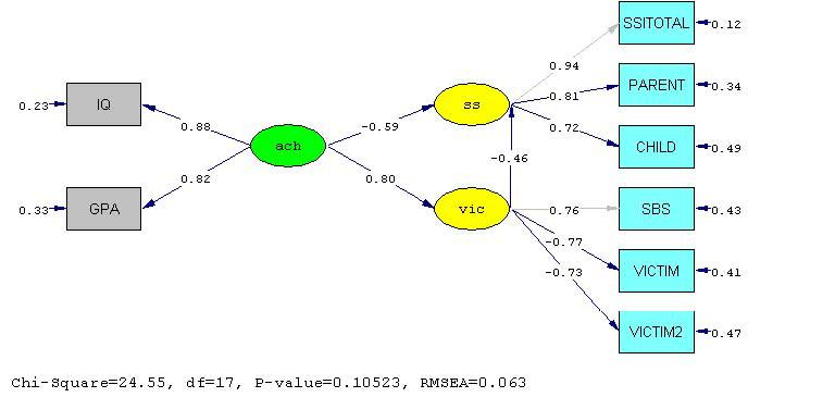
The path diagram with standardized estimates is produced in the final step in the analysis. Note that all direct effects are significant with the exception of SS to SSITOTAL and the latent variable relating vic to SBS. The latent variable SS reflects estimates of child and parent indications about severity of the problem, but not clinical indications about severity of stuttering. The model indicates that both achievement and victimization influence severity of stuttering, and that achievement has both a direct effect on severity of stuttering and an indirect effect that is mediated by victimization. This model was estimated using a covariance matrix with maximum likelihood estimation. It appeared to fit the data relatively well (according to the criteria of Hu & Bentler, 1999) although it is limited by the small sample size (χ² = 24.55, df=17, P =0.11, RMSEA=0.06; Standardized RMR = 0.03, CFI = 0.99, NNFI = 0.98).

Appendix B

Fictitious data compiled for modeling purposes only. These are included so that readers may reproduce the results or practice developing different forms of SEM analysis.

SSI = clinical assessment of stuttering severity - high scores = more severe; Parent = parent report of stuttering severity - high scores = more severe; Child = child report of stuttering severity - high scores = more severe; IQ = score on the Otis-Lennon Mental Abilities Test; GPA = grade point average; SBS (social behavior at school checklist) = teacher report of bullying - low scores = more bullying; Victim1 = peer reports of bullying - high scores = more nominations as bully victim; Victim2 = parent report of bullying - high score = more bullying.

SSI	Parent	Child	IQ	GPA	SBS	Victim1	Victim2
30	27	28	79	1.67	29	1	2
23	21	20	108	4.00	38	1	1
14	10	11	131	3.75	42	0	1
25	10	25	100	2.50	40	2	1
18	20	19	107	3.50	41	1	1
12	13	17	115	4.00	42	0	1
15	14	19	92	2.23	42	1	2
8	10	8	111	3.00	41	1	1
9	17	17	95	3.00	40	0	1
6	14	13	106	3.75	41	0	1
9	9	9	107	3.00	42	1	2
29	25	22	88	2.25	38	3	3
19	18	15	109	2.25	42	1	3
19	14	8	102	2.75	40	2	1
25	20	34	81	2.00	39	3	2
36	23	20	93	2.00	35	7	2
19	17	18	106	2.75	38	1	1
30	20	20	97	2.67	25	4	5
21	10	20	112	3.00	42	2	2
12	15	15	95	2.75	40	0	1
29	39	33	86	1.00	33	1	2
24	34	22	90	2.50	40	0	3
15	18	13	118	3.00	42	1	2
13	20	21	115	3.75	42	0	1
11	19	16	105	2.75	40	0	1
22	26	18	81	1.50	41	5	2
35	35	26	83	.67	30	6	3
27	22	29	85	1.75	40	1	3
24	19	25	83	2.75	38	0	5
20	19	16	105	2.50	39	1	1
8	18	20	115	4.00	42	1	2
29	24	30	102	2.75	42	3	3
28	32	17	81	1.50	40	3	2
16	13	15	118	3.00	40	1	2
9	17	15	120	4.00	42	0	1
8	13	11	129	3.75	41	1	2
11	19	9	111	3.00	40	0	2
19	20	10	100	2.50	35	0	2
11	17	22	109	2.25	40	1	1
25	25	29	81	2.00	39	1	1
12	20	17	112	3.00	42	1	2
31	22	18	93	2.00	40	2	1
29	30	22	86	1.00	36	5	3
30	26	24	85	2.50	32	5	3
18	25	12	97	2.67	42	1	1
37	23	22	85	1.75	31	7	2
28	26	22	79	1.67	35	3	4
20	19	15	95	3.00	42	2	4
33	26	24	90	2.50	40	7	2
34	27	24	83	.67	39	8	2
34	25	22	92	2.23	38	4	3
16	14	19	115	3.75	42	2	2
28	26	22	88	2.25	40	2	2
18	10	13	106	2.75	42	2	1
10	15	13	108	4.00	41	0	1
11	14	11	115	3.75	41	0	2
17	19	16	106	3.75	40	2	3
25	27	23	124	2.00	37	6	3
24	27	14	95	2.75	36	2	3
25	15	13	85	2.75	32	2	4
22	19	21	99	3.50	42	1	2
28	24	21	99	2.67	40	8	3
28	22	21	95	2.75	36	4	3
25	24	18	92	3.50	39	2	2
36	32	25	83	2.75	30	9	5
22	20	19	95	1.50	40	2	2
25	23	21	92	2.23	39	4	3
23	21	15	105	2.75	35	1	2
30	24	23	85	1.50	34	2	3
8	15	16	115	4.00	42	0	1
14	17	15	111	3.00	42	4	1
18	16	18	112	3.00	41	1	2
11	15	17	118	3.00	42	0	2
23	18	14	100	2.50	36	0	3
25	32	21	95	1.50	36	2	3
27	22	23	88	2.25	31	1	2
24	27	26	86	1.00	42	0	2
29	30	22	85	1.75	40	4	3
10	13	17	115	3.75	42	1	1
8	10	12	129	3.75	41	0	2
15	22	11	106	2.75	40	2	1
31	24	21	90	2.50	30	10	4
15	25	23	99	3.00	41	4	2
34	28	23	81	2.00	31	9	5
32	35	25	79	1.67	33	6	4
30	28	24	93	2.00	40	5	3
18	19	18	109	2.25	42	2	2
26	25	23	83	2.75	40	4	3
28	26	23	85	2.50	38	6	2
26	25	17	85	2.75	40	3	3
33	30	25	83	.67	35	5	4
19	20	20	105	2.75	42	4	1
19	16	18	115	3.00	40	0	2
18	20	19	115	3.00	39	1	1
31	29	25	83	.67	31	6	6
9	15	18	115	4.00	42	1	1
25	22	22	99	3.00	40	2	2
11	19	15	115	4.00	42	0	2
12	15	16	115	3.75	42	0	3
24	21	21	99	2.75	41	4	2
29	26	22	88	2.25	40	5	3
23	20	19	109	2.25	38	2	2
26	22	22	100	2.50	35	0	3
40	32	29	85	1.75	29	10	6
30	25	22	93	2.00	37	6	5
31	22	22	90	2.50	36	5	2
20	15	18	118	3.00	41	0	1
30	33	23	95	1.50	35	0	4
29	22	23	92	3.50	38	5	3
28	30	21	92	2.23	38	4	3
35	29	30	86	1.00	30	8	4
25	19	22	97	2.67	40	2	2

References

- Baron R90M, Kenny DA. The moderator-mediator variable distinction in social psychological research: Conceptual, strategic and statistical considerations. Journal of Personality and Social Psychology. 1986;51:1173–1182. doi: 10.1037//0022-3514.51.6.1173. [DOI] [PubMed] [Google Scholar]
- Bentler PM. Comparative fit indices in structural models. Psychological Bulletin. 1990;107:238–246. doi: 10.1037/0033-2909.107.2.238. [DOI] [PubMed] [Google Scholar]
- Boomsma A. Reporting analyses of covariance structures. Structural Equation Modeling: A Multidisciplinary Journal. 2000;7:461–483. [Google Scholar]
- Browne MW, Cudeck R. Alternative ways of assessing model fit. In: Bollen KA, Long JS, editors. Testing Structural Equation Models. Beverly Hills, CA: Sage; 1993. [Google Scholar]
- Cheung GW, Rensvold RB. Evaluating goodness-of-fit indexes for testing measurement invariance. Structural Equation Modeling. 2002;9:233–255. [Google Scholar]
- Cliff N. Some cautions concerning the application of causal modelling methods. Multivariate Behavioral Research. 1983;18:115–126. doi: 10.1207/s15327906mbr1801_7. [DOI] [PubMed] [Google Scholar]
- Cudeck R. Analysis of correlation matrices using covariance structure models. Psychological Bulletin. 1989;105:317–327. [Google Scholar]
- Earley PC, Lituchy TR. Delineating Goal and Efficacy Effects: A Test of Three Models. Journal of Applied Psychology. 1991;76:81–98. [Google Scholar]
- Farrell AD, Sullivan TN. Structure of the Weinberger Adjustment Inventory Self-Restraint Scale and its relation to problem behaviors in adolescence. Psychological Assessment. 2000;12:394–401. [PubMed] [Google Scholar]
- Furnham A, Davies S. Involvement of social factors in stuttering: A review and assessment of current methodology. Stammering Research. 2004;1:112–122. [PMC free article] [PubMed] [Google Scholar]
- Fife-Schaw C. Introduction to Structural Equation Modeling. In: Breakwell GM, Hammond S, Fife-Schaw C, editors. Research Methods in Psychology. Second Edition London: Sage; 2000. [Google Scholar]
- Gerbing DW, Anderson JC. An updated paradigm for scale development incorporating unidimensionality and its assessment. Journal of Marketing Research. 1988;25:186–192. [Google Scholar]
- Hayduk LA, Glaser DN. Jiving the four step, waltzing around factor analysis and other serious fun. Structural Equation Modeling. 2000;7:1–35. [Google Scholar]
- Hershberger SL. The Growth of Structural Equation Modeling: 1994-2001. Structural Equation Modeling. 2003;10:35–47. [Google Scholar]
- Hoyle RH. The Structural Equation Modeling Approach: Basic concepts and fundamental issues. In: Hoyle RH, editor. Structural equation modeling: Concepts Issues and Applications. London: Sage; 1995. pp. 1–18. [Google Scholar]
- Hoyle RH, Panter . Writing about structural equation models. In: Hoyle RH, editor. Structural equation modeling: Concepts Issues and Applications. London: Sage; 1995. pp. 158–176. [Google Scholar]
- Hu L, Bentler PM. Evaluating model fit. In: Hoyle RH, editor. Structural Equation Modeling: Concepts Issues and Applications. London: Sage; 1995. pp. 76–99. [Google Scholar]
- Hu L, Bentler PM. Fit indices in covariance structure modeling: Sensitivity to underparameterized model misspecification. Psychological Methods. 1998;3:424–453. [Google Scholar]
- Hu L, Bentler PM. Cutoff criteria for fit indexes in covariance structure analysis: Conventional criteria vs. new alternatives. Structural Equation Modeling. 1999;6:1–55. [Google Scholar]
- Jaccard J, Wan CK. Measurement error in the analysis of interaction effects between continuous predictors using multiple regression: Multiple indicator and structural equation approaches. Psychological Bulletin. 1995;116:348–357. [Google Scholar]
- Jöreskog KG. A general approach to confirmatory maximum likelihood factor analysis. Psychometrika. 1969;34:183–202. [Google Scholar]
- Jöreskog KG. Simultaneous factor analysis in several populations. Psychometrika. 1971;36:409–426. [Google Scholar]
- Jöreskog K, Sörbom D. LISREL 8: User's reference guide. Hillsdale, NJ: Lawrence Erlbaum Associates; 1996. SSI Scientific software International. [Google Scholar]
- Kline RB. Principles and Practice of Structural Equation Modeling. Second Edition NY: Guilford Press; 2004. [Google Scholar]
- Kolk H, Postma A. Stuttering as a covert repair phenomenon. In: Curlee RF, Siegel G, editors. Nature and treatments of stuttering: New directions. Needham Heights, MA: Allyn & Bacon; 1997. [Google Scholar]
- Levine SZ, Jackson CJ. Eysenck's theory of crime revisited: Factors or primary scales? Legal and Criminological Psychology. 2004;9:135–152. [Google Scholar]
- Little TD, Cunningham, Shahar G, Widaman KF. To parcel or not to parcel: Exploring the question, weighing the merits. Structural Equation Modeling. 2002;9:151–173. [Google Scholar]
- MacCallum RC, Wegener DT, Uchino BN, Fabrigar LR. The problem of equivalent models in applications of covariance structure analysis. Psychological Bulletin. 1993;114:185–199. doi: 10.1037/0033-2909.114.1.185. [DOI] [PubMed] [Google Scholar]
- MacCallum RC, Widaman KF, Zhang S, Hong S. Sample size in factor analysis. Psychological Methods. 1999;4:84–99. [Google Scholar]
- Maruyama GM. Basics of Structural Equation Modeling. Thousand Oaks: Sage; 1998. [Google Scholar]
- Moulder BC, Algina J. Comparison of methods for estimating and testing latent variable interactions. Structural Equation Modeling. 2002;9:1–19. [Google Scholar]
- Mulaik SA, Millsap RE. Doing the four step right. Structural Equation Modeling. 2000;7:36–73. [Google Scholar]
- Munck IM. Model building in comparative education : Application of the LISREL method to cross-national survey data. Stockholm: Almqvist & Wiksell; 1979. (International Association for the Evaluation of Educational Achievement Monograph Series, No. 10). [Google Scholar]
- Muthén B. Beyond SEM: General latent variable modeling. Behaviormetrika. 2002;29:81–117. [Google Scholar]
- Olsson UH, Foss T, Troye SV, Howell RD. The performance of ML, GLS, and WLS estimation in structural equation modeling under conditions of misspecification and nonnormality. Structural Equation Modeling. 2000;7:557–595. [Google Scholar]
- Quintana SM, Maxell SE. Implications of recent developments in structural equation modeling for counseling psychology. The Counseling Psychologist. 1999;27:485–587. [Google Scholar]
- Petrides KV, Furnham A, Jackson CJ, Levine SZ. Exploring issues of personality measurement and structure through the development of a revised short form of the Eysenck Personality Profiler. Journal of Personality Assessment. 2003;81:272–281. doi: 10.1207/S15327752JPA8103_10. [DOI] [PubMed] [Google Scholar]
- Raykov T, Marcoulides GA. On desirability of parsimony in structural equation model selection. Structural Equation Modeling. 1999;6:292–300. [Google Scholar]
- Raykov T, Marcoulides GA. Can there be infinitely many models equivalent to a given covariance structure model? Structural Equation Modeling. 2001;8:142–149. [Google Scholar]
- Riley GD. The Stuttering Severity Instrument for Adults and Children. third edition Austin, TX: Pro-Ed; 1994. [Google Scholar]
- Schumacker RE. Latent variable interaction modeling. Structural Equation Modeling. 2002;9:40–54. [Google Scholar]
- Smith A. Stuttering: A unified approach to a multifactorial dynamic disorder. In: Bernstein Ratner N, Healey EC, editors. Stuttering research and practice: Bridging the gap. Mahwah: Lawrence Erlbaum Associates; 1999. [Google Scholar]
- Smith A, Kleinow J. Kinematic correlates of speaking rate changes in stuttering and normally fluent adults. Journal of Speech, Language, Hearing Research. 2000;43:521–536. doi: 10.1044/jslhr.4302.521. [DOI] [PubMed] [Google Scholar]
- Werts CE, Rock DR, Linn RL, Jöreskog KG. A general method of estimating the reliability of a composite. Educational and Psychological Measurement. 1978;38:933–938. [Google Scholar]
- Wright S. The method of path coefficients. Annals of Mathematical Statistics. 1934;5:161–215. [Google Scholar]