Realistic Simulation of the 3D Growth of Brain Tumors in MR Images Coupling Diffusion with Biomechanical Deformation

Abstract

We propose a new model to simulate the 3D growth of glioblastomas multiforma (GBMs), the most aggressive glial tumors. The GBM speed of growth depends on the invaded tissue: faster in white than in gray matter, it is stopped by the dura or the ventricles. These different structures are introduced into the model using an atlas matching technique. The atlas includes both the segmentations of anatomical structures and diffusion information in white matter fibers.

We use the finite element method (FEM) to simulate the invasion of the GBM in the brain parenchyma and its mechanical interaction with the invaded structures (mass effect). Depending on the considered tissue, the former effect is modeled with a reaction-diffusion or a Gompertz equation, while the latter is based on a linear elastic brain constitutive equation. In addition, we propose a new coupling equation taking into account the mechanical influence of the tumor cells on the invaded tissues. The tumor growth simulation is assessed by comparing the in-silico GBM growth with the real growth observed on two magnetic resonance images (MRIs) of a patient acquired with six months difference. Results show the feasibility of this new conceptual approach and justifies its further evaluation.

I. INTRODUCTION

A. Motivation

The majority of the primary tumors of the central nervous system are from glial origin, among which the glioblastomas multiforma (GBMs) are the most aggressive. Despite the substantial research effort against these pathologies, patients treated with state-of-the-art therapy at Centre Antoine Lacassagne have a median survival of approximately 1 year.

Relatively little progress has been made toward the construction of a general model describing the growth of these tumors. The interest to carry out a simulation of the tumor growth is multiple. First, it provides a better understanding of the physiology of the tumor growth. Second, it could help predict the tumor evolution from a limited number of time patient observations. Third, solving an inverse problem based on this model could be used to quantify the tumor aggressiveness in a given patient. Last, such a model could improve therapy planning (in surgery or radiotherapy) by better defining the invasion margins based on the local estimation of the tumor cell density.

A primary objective of our model is to investigate the 3D invasion of brain tumors and in particular the respective influence of the tumor diffusion and mass effect. The work reported in this paper, including a case study, should be seen as a proof-of-concept toward this goal.

B. Assessing the Tumor Growth Rate

The invasion speed of some lesions can be more important than others, due to a greater ”aggressiveness”. From a time series of MR images, it is possible to picture the 3D invasion of GBM in the brain [1]. Since tumors can exhibit different rates of growth, it is then possible to find the best model parameters -that best match the predicted with the observed invasion- to characterize the local or global tumor aggressiveness. In other words, aggressiveness can be considered as one of the hidden parameters of the model and could be estimated by solving the following inverse problem: given a time series of images, the hidden parameters can be estimated as those resulting in the most realistic simulation with respect to the data.

C. Therapy Planning

In radiotherapy treatments, the delineation of the Clinical Target Volume (CTV) has to take into account the presence of isolated malignant cells in the area surrounding the edema. Such malignant cells cannot be seen in a T2-weighted MR image. By estimating a tumor cell density, our approach could help to estimate the risk of finding isolated malignant cells outside the edema, and thus can help to delineate the CTV.

Furthermore, the segmentation of the Gross Tumor Volume 1 and 2 (GTV1 and GTV2, see Section II-C for a short description of the GTV classification and [2] for further details) is performed on a MR image acquired before therapy. Because a significant delay may occur between the image acquisition and the radiotherapy treatment, our tumor model could predict the additional tumor invasion at the treatment time.

Once a patient with a GBM has been treated, the recurrence occurs on average one year later. Radio-necrosis, which is a radiotherapy complication, has the same signal in MRI as the tumor recurrence, but its growth law is different. Here again, a numerical model could be used to discriminate radio-necrosis from tumor recurrence.

Finally, we believe that an in-silico tumor growth model could be of great interest for neurosurgeons since they have to estimate the trade-off between risks and benefits of surgical procedures. Indeed, the combination of a functional atlas with the tumor simulation could help predicting future functional impairments upon the tumor invasion in the patient’s brain.

II. PREVIOUS WORK AND CONTRIBUTIONS

A. Tumor Growth Models

Without loss of generality, tumor growth models can be classified into two categories depending on their observation scale:

• Cellular and microscopic models. These models describe the cellular division speed. Basic models consider the behavior of isolated cells (exponential, Gompertz), while more complex models take into account the interaction between the cells and their environment (cellular automata).

• Macroscopic models. These models describe the evolution of the local tumor cell density. Most of these models rely upon a reaction-diffusion equation to account for the tumor propagation.

1) Exponential

The first work on an exponentially growing population was performed by Reverend T.R. Malthus in 1798. The exponential growth is the simplest proliferation law. It describes the population density N(t) at any time t as a function of the initial population density N(0) and the constant growth rate k: N(t) = N(0)e^kt. k depends on the intrinsic aggressiveness of the tumor. This function is better suited for quantifying the growth of small tumors during a short time [3].

2) Gompertz

Malthus work was later modified, in particular by Gompertz (1825). Beyond a certain size, the exponential growth gradually slows down to reach a Malthusian asymptotic limit N_∞. The initial exponential growth characterised by its growth rate k is later limited to an asymptotic rate:

$$\frac{\partial N}{\partial t}=kN\text{ln}\left(\frac{N_{\infty }}{N}\right)\{k,N_{\infty }\}>0$$ (1)

The so-called ”Gompertz Growth Law” has been used to describe the growth rate of solid avascular tumors at the population level and succeeded in specific clinical application [4], [5].

3) Cellular Automata

Since the Gompertz and the exponential models do not take the interactions between cells and tissues into account, they are good approximations for the initial microscopic tumor growth only. The cellular automata models make the link between the microscopic proliferation and the macroscopic diffusion models.

This approach differs from deterministic approaches because it computes each division and interaction at a cell scale to simulate the macroscopic behavior of the tumor growth. Cellular automata are used to simulate the early growth of the tumors and to examine their early vascularization and metabolism.

The cells and micro-vessels affect the extra-cellular concentration which, in turn, affect back the evolution of each automaton [6]. Complex models take into account the development of the social behavior, expressed in the co-operative cellular movement [7]. Some cellular automata are available on the Internet¹.

4) Diffusive Models

On the one hand, the exponential and Gompertz cellular models represent a good approximation of the microscopic behavior of the GTV1 in the GBM, which is not really affected by the nature of the surrounding tissue. On the other hand, the macroscopic diffusive component of the GBM depends on the nature of the brain tissue. Recent attempts have been made to model this infiltrating component, taking into account local diffusivity parameters.

The diffusive models propose a macroscopic way of considering the tumor growth. Major contributions in this domain refer to the reaction-diffusion formalism introduced by Murray in the early 1990 and later formulated as a conservation equation [8], [9]:

$$\frac{\partial c}{\partial t}=-\mathit{\text{div}}(\underset{¯}{J})+S(c,t)-T(c,t)$$ (2)

• c represents the tumor cell density.

• J̲ represents the diffusion flux of tumor cells², which we assume to obey Fick’s law, i.e. the diffusion flux of cell is proportional to the gradient of tumor cell density:

  $$\underset{¯}{J}=-D_T\underset{¯}{▽c}$$ (3)

  D_T is the diffusion coefficient of tumor cells.

• S(c, t) represents the source factor function, describing the proliferation of tumor cells.

• T(c, t) is used to model the efficacy of the tumor treatment.

This diffusion equation is the basis of major contributions related to diffusive tumor models [10], [9]. Other models [11] include the mechano-chemical aspect of cell mobilities by including an active mobility term in the reaction-diffusion equation.

B. GBM Tumor Growth

1) Classification and Mortality

Glioblastomas can be classified as primary or secondary. Primary GBMs represent the majority of cases (60%), more frequent in older patients (> 50 years). Secondary GBMs typically develop in younger patients (< 45 years) through malignant progression from a low-grade astrocytoma. This progression shows a large variability, from 1 to 10 years. Whereas both are classified as glioblastomas, there is increasing evidence that primary and secondary GBMs evolve as distinct diseases.

Despite the substantial research effort toward improving tumor treatment, no significant advances in the treatment of GBMs have occurred in the past 25 years. Without therapy, patients with GBMs usually die within 10 months. Patients treated with state-of-the-art therapy, including surgical resection, radiation therapy, and chemotherapy, have a median survival of approximately 1 years [12]. To date, there is no evidence that patients with a secondary GBM have a better prognosis than patients with a primary GBM.

2) Glioblastoma Models

Previous publications focusing on GBM models isolate two key characteristics: a proliferation component and a diffusion component [11], [9], [13], [14]. These two characteristics can be related to the categories described in Section II-A: the proliferation component often corresponds to the central active part of the tumor and can be described with a cellular proliferation law. The diffusion component is generally associated to the external part of the tumor and can be described by a diffusion law. GBMs can thus be described as a combination of two different growth models depending on the considered tumor area (central active or external).

C. Contributions

In this paper, we propose a patient-specific simulator of GBM growth, including the brain deformation (mass effect) induced by the tumor invasion. The simulation relies on a model discretized with the Finite Element Method (FEM) initialized from the patient MRIs. Additional structures (such as the white matter fiber directions, gray matter) have been included in the patient model using an atlas.

Furthermore, we propose to make the link between the radiotherapy classification of tumors in Gross Tumor Volumes (GTV) proposed in some protocols for radiotherapy treatment [2] and the two distinct invasion behaviors:

• The GTV1 is associated with the expansion component. Because it does not infiltrate the tissue, this proliferation is directly correlated with a volume increase. By creating new cells, the GTV1 pushes away the surrounding structures. It is therefore responsible for the major mechanical mass effect. For instance, the GTV1 volume increase is described in our model by an exponential law.

• The GTV2 is associated with the diffusion component. It invades adjacent structures by a diffusion process and is responsible for the infiltration in white and gray matter. This diffusion component expands faster than the GTV1 but exhibit little mass-effect. The GTV2 is thus described in our model with a reaction-diffusion equation. In addition, we propose to model the associated mass effect with a coupling equation which links the mechanical to the diffusion process.

An example of the usual GTV segmentation can be seen on Figure 1. The model is initialized using a standard segmented patient MRI.

Fig. 1.

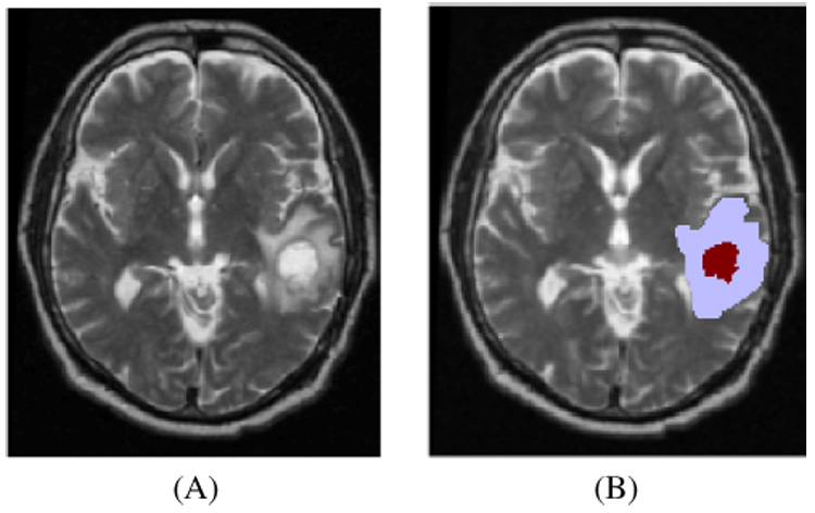
MR images of a patient (A) T2; (B) GTV1 (dark red) and GTV2 (light blue) segmentations overlaid on the T2 MRI.

Compared to the previous publications dealing with the tumor growth modeling problem ([10], [9], [15]), our approach includes several improvements:

• The use of diffusion tensor imaging to take into account the anisotropic diffusion process in white matter fibers (as opposed to the isotropic reaction-diffusion formalism of Swanson et al. [9]).

• The use of the radiotherapy volume classifications to initialize the source of the diffusion component (as opposed to point sources in [9]).

• A new coupling equation between the reaction-diffusion and the mechanical constitutive equation to simulate the mass-effect during of the virtual glioblastoma (VG) growth.

• The initialization with a patient’s tumor and a quantitative comparison with the observed invasion in the later patient MR images.

III. GLIOBLASTOMA GROWTH SIMULATION

A. Overview of the Method

Our GBM growth simulation consists of two coupled models:

1. A model of the multiplication and diffusion of the tumor that describes the evolution of the tumor density c over time in the brain.

2. A model of the expansion of the tumor that predicts the mass effect induced by both the tumor proliferation and infiltration.

The coupling between these two models is further described in Section III-D.2.b but it assumes the following behavior: the mass effect is directly related to the tumor density c but c is not influenced by the mass effect.

This simple coupling leads to a four step algorithm described in Figure 2:

• Image segmentation and registration. The two gross volumes - GTV1 and GTV2 - are manually delineated by an expert (who regularly segments these tumors in MR images for clinical radiotherapy treatments) from the patient MR images. The patient MR images (both March and September) are registered with respect to an anatomical atlas. This atlas includes for each voxel the location of the main cerebral structures and diffusion tensors in the white matter.

• Meshing and Initialization. A tetrahedral mesh of the patient’s brain is built based on the anatomical segmentation of the patient image registered in the atlas reference frame. Tissue properties are assigned to their associated tetrahedra using the atlas. Furthermore, the value of the tumor density c is initialized based on the GTV1 and GTV2 segmentations by interpolating between the two boundaries.

• Simulation. The simulation of the VG diffusion and expansion is performed following the mechanical and diffusion equations discretized with the finite element method.

• Comparison. At the end of the growth process, the simulated deformations are applied to the registered March images of the patient. Then, the relevance of the model is evaluated by comparing both the predicted tumor iso-density contours and the brain deformation with the registered patient MR images acquired six months later.

Fig. 2.

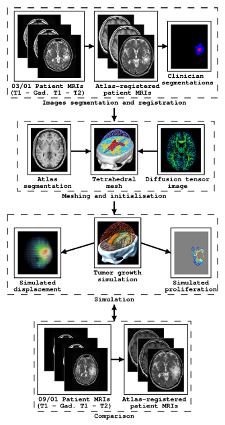
Flowchart of the proposed approach

To make the registration and the computation more accurate, we chose to make all computations in the anatomical atlas space since it has the largest image resolution. Every patient image (March and September) is thus registered to the anatomical atlas image. In addition, we introduce the diffusion information through the registration of a DTI to the anatomical atlas. The registration of pathological to healthy subject images is still an open problem and there is no validated non-rigid registration algorithm considered as a gold-standard. However some authors proposed different approaches aiming at limiting the tumor-induced deformation artifacts. For example, the approach of Dawant et al. [16] corrects the mass effect induced by the volume variation of tumors. However, this method is not suited for GBMs, also showing a diffusion component involving mechanical deformations. We chose to solve this problem using an affine transformation which limits the number of degrees of freedom. Ultimately, the complete simulation could be performed in the patient space with a high resolution anatomical MRI and a DTI of the patient.

B. Pre-Processing of MR Images

1) Patient

The standard imaging protocol for brain tumor radiotherapy has been used for this study. Three sequences, T1, T2, and T1 with gadolinium injection (exported in Dicom-3 format) were used. Two different MRI series of the same patient were acquired with 6 months difference (Figure 3). The size and format of the images are shown in Table I. These MRIs have been acquired in the standard follow-up, after surgical resection, radiotherapy treatment and/or chemotherapy [17]. No treatment was administrated for the recurrent GBM before clinical symptoms appeared (in September for the considered patient).

Fig. 3.

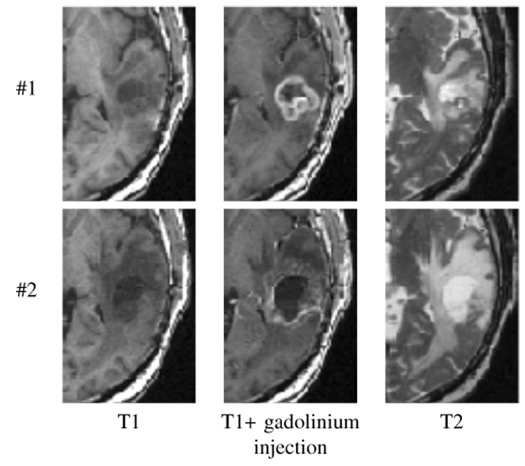
Close up view of the tumor region on the first (#1), and second (#2) MRI series (T1 − T1 + gadolinium injection − T2), acquired respectively in March and September 2001.

TABLE I.

MRIs CHARACTERISTICS

	Image size	Voxel size (mm)
Patient MRI T1	256*256*60	1.015*1.015*2
Patient MRI T2	256*256*64	1.015*1.015*1.9
Atlas MRI T1	181*217*181	0.6*0.6*0.6
Atlas MRI T2	181*217*181	0.6*0.6*0.6
Atlas DTI	256*256*36	1.0*1.0*4.0

2) Tumor Segmentation

The initial tumor location is used to set the boundary conditions of our model. This was performed manually by a medical expert using the three acquisition modalities. Because the external ring of the Gross Tumor Volume 1 (GTV1) represents the most active part of the tumor, it is enhanced by gadolinium. Its boundary is defined as the area of contrast enhancement observed on the T1-weighted MRI following gadolinium injection. The GTV2 takes into account the probability of presence of isolated malignant cells in the edema surrounding the tumor. Its boundary is delimited by the area of hyper-signal in the T2-weighted MRI.

3) Registration

All images (patient acquisitions in March and September, DTI) have been registered to the anatomical atlas image. Thus two distinct affine registrations have been performed to:

• register the DTI image to the anatomical atlas. The transformation was first estimated between the anatomical atlas and the T2 weighted MR image acquired in the same space as the diffusion gradient images. Once measured, we applied the transformation to the diffusion tensor image to get the tensors in the anatomical atlas space.

• register the patient images to the anatomical atlas. The transformation was estimated between the anatomical atlas and the T2 weighted MR image of the patient (both September and March). The transformation is then applied to every image of the patient to register them in the anatomical atlas space.

Every registration is computed using the Baladin software [18]. This algorithm computes the transformation in three steps in a coarse to fine approach:

• Estimate the displacements $\underset{¯}{d}(\underset{¯}{X_i})$ of a domain V composed of voxels centered in $\underset{¯}{X_i}$ ($\underset{¯}{X_i}\in V$ starting with the full image) from the reference image to the target image based on a block matching approach. In our case, we use the sum of squared differences as a similarity measure, since both images are the same image modality.

• Find the optimal affine transformation T̲ (X̲) = F̳X̲ + C̲ that minimizes the distance error with respect to the measured displacements $\underset{¯}{d}(\underset{¯}{X_i})$:

  $$\underset{¯}{T}=\text{arg}\underset{T}{\text{min}}\left({\displaystyle \sum _{\underset{¯}{X_i}\in V}\parallel \underset{¯}{T}(\underset{¯}{X_i})-\underset{¯}{d}(\underset{¯}{X_i}){\parallel }^2}\right)$$ (4)

• Discard the outliers using a least trimmed square estimator [19].

To obtain a better matching between deep brain structures, we removed the skull from both images and compute the transformations on brains only.

4) Building an Atlas

An atlas usually consists of an anatomical MR image and an associated label for each voxel representing the nature of the tissue. In our case, we propose to add a diffusion tensor information to the white matter fiber labeled voxels. Therefore, this atlas was built from two images: a labeled MR image used as an anatomical atlas, and a diffusion tensor image registered with the anatomical MRI.

a) Anatomical Atlas

We used a fully artificial MRI for the anatomical atlas, generated by the ”brainweb” software [20]. The delineation of the structures is then performed with different thresholds on this MRI [21]. However an asymmetry exists and can introduce a bias. Thus we mirrored the right part of the head to generate a perfectly symmetrical atlas MRI (see Figure 4). Artificial MRI characteristics are shown in Table I. We focused on different structures of interest for the purpose of tumor growth simulation: skull, ventricular system, brain (gray matter and white matter) and falx cerebri (see Figure 4). This atlas is used to segment the image of the patient acquired in March.

Fig. 4.

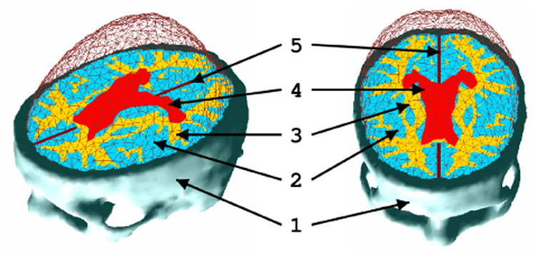
Visualization of the brain surface mesh and the different structures included in the model: (1) the skull, (2) gray matter, (3) white matter, (4) ventricles, (5) falx cerebri.

b) Diffusion Tensor Information

The GBM is a tumor of glial origin and grows preferentially in the white matter fiber directions [22]. To take this fact into account and to be more accurate in both direction and speed of progression of the tumor, data from Diffusion Tensor Imaging (DTI) was used in the white matter.

The DTI measures the variance of the conditional probability $P(\underset{¯}{X}|\underset{¯}{X_0},t)$, which represents the probability of finding a water molecule at a position X̲ and at time t given its original position $\underset{¯}{X_0}$:

$$\langle (\underset{¯}{X}-\underset{¯}{X_0})·{(\underset{¯}{X}-\underset{¯}{X_0})}^T\rangle =6\underset{¯}{\underset{¯}{D_w}}t$$ (5)

Where 〈Y〉 stands for Expectation(Y).

This DTI is reconstructed from n diffusion gradient images (n ≥ 6) and a null gradient image (T2 weighted). This diffusion is about 2.9 × 10⁻³ mm² s⁻¹ in pure water and three times larger in the fiber direction (1.2 × 10⁻³ mm² s⁻¹) than in the transverse direction 0.4 × 10⁻³ mm² s⁻¹ [23].

Different methods have been proposed in the literature to apply an affine transformation to a diffusion tensor image. Alexander et al. [24] proposes 3 methods (no re-orientation, local rigid and preservation of principal components), suggesting to use the third method for multi-subject non rigid registration of soft tissue. In addition to the local rigid strategy, Sierra [23] also proposes a local affine and a local affine without scaling re-orientation strategy, arguing in favor of the local rigid strategy. Xu. et al. [25] proposed a re-orientation strategy based on a statistical estimation of the local fiber orientation. It seems however that there is no real consensus on the right method to use to warp tensors. We chose to apply the affine transformation without scaling, following [23] which seems to best account for shearing while preserving the volume of the tensor. However, further experiments are definitely needed to confirm the validity of this choice. Using notations defined in Section III-B.3 for the affine transformation, the registered diffusion tensor image $\underset{¯}{\underset{¯}{D{\prime }_w}}$ is mathematically defined as:

$$\underset{¯}{\underset{¯}{D{\prime }_w}}(\underset{¯}{X_0})=\underset{¯}{\underset{¯}{F}}\left[\underset{¯}{\underset{¯}{D_w}}({\underset{¯}{\underset{¯}{F}}}^{-1}(\underset{¯}{X_0}-\underset{¯}{C}))\right]{\underset{¯}{\underset{¯}{F}}}^T$$ (6)

We require that the affine registration process does not change the underlying tissue absolute diffusivity properties. Following the original idea of Sierra [23], the final diffusion tensor is normalized by the transformation scaling factor det(F̳)², so that det(D̳) = det(Dʹ̳).

The tensor registration is decomposed in three steps:

• Finding the affine transformation T which displaces a voxel at position X̲ taken in the T2 weighted MRI from the original patient DTI dataset to the position $\underset{¯}{X\text{'}}=\underset{¯}{T}(\underset{¯}{X})=\underset{¯}{\underset{¯}{F}}\underset{¯}{X}+\underset{¯}{C}$ in the atlas image.

• Compute $\underset{¯}{\underset{¯}{{{\displaystyle D}}_w^{*}}}=\underset{¯}{\underset{¯}{D_w}}({\underset{¯}{\underset{¯}{F}}}^{-1}(\underset{¯}{X_0}-\underset{¯}{C}))$ which corresponds to registering each gradient image in the atlas geometry.

• Compute $\underset{¯}{\underset{¯}{D{\prime }_w}}(\underset{¯}{X_0})=\frac{1}{\mathit{\text{det}}{(\underset{¯}{\underset{¯}{F}})}^2}\underset{¯}{\underset{¯}{F}}\underset{¯}{\underset{¯}{D{*}_w}}{\underset{¯}{\underset{¯}{F}}}^T$.

C. Growth of the Tumor: Evolution of the Tumor Cell Density

1) Diffusion Equation

We rely on the reaction-diffusion model (Equation 2) to account for the growth and the spreading of tumor cells in the brain parenchyma outside the GTV1. The GTV1 is used as a source-volume for the diffusion of tumor cells. This volume is thus a fixed boundary condition of our model, which tumor cell density c is equal to the maximum tumor cell carrying capacity of the brain parenchyma C_max, estimated to be equal to 3.5 × 10⁴ Cells mm⁻³ [26], [14]. Since the purpose is only to simulate the tumor growth before (or without) treatment, we will not model the treatment term T(c, t). Consequently, the images we chose for the simulation were acquired before the first clinical symptoms appeared and before starting the radio-therapy and chemo-therapy treatment. In addition we propose to model the anisotropy of malignant tumor cell diffusion in the white matter considering a diffusion tensor $\underset{¯}{\underset{¯}{D_t}}$:

$$\underset{¯}{J}=-\underset{¯}{\underset{¯}{D_t}}\underset{¯}{▽c}$$ (7)

$\underset{¯}{\underset{¯}{D_t}}$ represents the local diffusivity of the tissue with respect to tumor cells and depends on the white matter fibers direction and the nature of the tissue.

Different equations can model the source factor S(c, t). For example, the gompertz law can be used:

$$S(c,t)=\rho c\text{ln}\left(\frac{C_{\mathit{\text{max}}}}{c}\right)$$ (8)

or the classical second order polynomial equation:

$$S(c,t)=\rho c\left(1-\frac{c}{C_{\mathit{\text{max}}}}\right)$$ (9)

leading to the Fisher reaction-diffusion equation. To minimize the number of tumor-intrinsic parameters, and to simplfy the model, we use a linear function to model the source factor, reflecting its aggressiveness:

$$S(c,t)=\rho c$$ (10)

Then combining Equations 10 and 7 with 2, we can express the reaction-diffusion law:

$$\frac{\partial c}{\partial t}=\mathit{\text{div}}\left(\underset{¯}{\underset{¯}{D_t}}\underset{¯}{▽c}\right)+\rho c$$ (11)

In this equation, c represents the normalized cell density. The real cell density C is obtained by multiplying c with the carrying capacity of the tissue C_max. As a consequence the tumor cell density is bounded between 0 and 1 (c ∈ [0, 1]), so that the increase of c is stopped when reaching the value 1. This implies a saturation effect, limiting the application of Equation 11 to the tumor density range c ∈ [0, C_max] and to the points of the brain located outside the GTV1. The local behavior of the tumor therefore only depends on the diffusion tensor $\underset{¯}{\underset{¯}{D_t}}$ and the source factor ρ.

To better understand the role of anisotropy in the diffusion process, we solved Equation 11 on two test-cubes (see Figure 5). In these examples, the tumor cell density is fixed to C_max for the central part of the tumor (initialized as a random shape, central blue part in the cube of Figure 5).

Fig. 5.

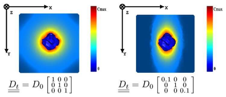
Behavior of the reaction-diffusion equation on test cases. (Left) isotropic. (Right) anisotropic. The tumor cell density is fixed to C_max for the central part of the tumor (initialized as a random shape, central blue part in the cube).

2) Model Parameters and Initialization

Because the diffusion process does not occur in the skull or in the ventricles, we only mesh the brain. We will see later that this mesh is also compatible with mechanical boundary conditions. Then, we propose the following characteristics for the model:

• Since the conductivity of the skull and the ventricles is null, the flux at the mesh surface should be zero. Therefore the boundary condition for the mesh surface is:

  $$\underset{¯}{J}·\overrightarrow{n}=0$$ (12)

• To the best of our knowledge, there exists no quantitative evaluation of the diffusion of tumor cells in white matter fibers. In particular, the comparison of the influence of anisotropy on the diffusion of water molecules versus tumor cells has not been studied yet. In this article, we assume that the anisotropic ratio of diffusion is the same for water molecules and tumor cells so that $\underset{¯}{\underset{¯}{D_t}}=\alpha \underset{¯}{\underset{¯}{D_w}}$ (α constant value). However, further experiments are needed to validate this hypothesis. Indeed, it could be that this relation may vary depending on the tumor aggressiveness. We use the previously described diffusion atlas (see Section III-B.4) to initialize the tumor cell diffusion tensor $\underset{¯}{\underset{¯}{D_t}}$ in white matter.

• There are several indications that GBMs diffuse more slowly in the gray matter than in the white matter [27]. The diffusivity in gray matter is thus chosen as a fraction of the maximum diffusivity in white matter $\beta =\frac{D_{\mathit{\text{gray}}}}{D_{\mathit{\text{white}}}}$, and isotropic. The intrinsic aggressiveness of the tumor is then controlled by two parameters α and β. β is adjusted to visually best simulate the in-silico diffusion of the GBM in gray matter for our patient: $\beta =\frac{1}{100}$.

• Because tumor cells cannot diffuse through the falx cerebri, we set the diffusivity of every tetrahedron crossing the falx to zero. One can notice on Figures 4, 6, 7 and 9 that the falx is not a simple plane between the two hemispheres, but tumor cells can actually diffuse from one hemisphere to the other across the corpus callosum.

• The GTV1 capacity is set to the maximum carrying capacity of the brain tissue C_max (3.5 × 10⁴ Cells mm⁻³).

• As discussed in [28], one cannot determine both α and ρ from two different instants only. We thus arbitrarily set $\rho =\frac{\eta }{100}$ (η is defined in Section III-D.1). The α parameter is then adapted to qualitatively fit the diffusion of the model with the images of the patient acquired 6 months later. We found α = 5 × 10⁻³, which leads to a maximum diffusion value of 10⁻⁵ mm² s⁻¹. This value is consistent with the diffusion value used in [9] (2 times smaller). However, inter-subject diffusion parameters are difficult to compare, since different tumors can have different diffusion properties.

Fig. 6.

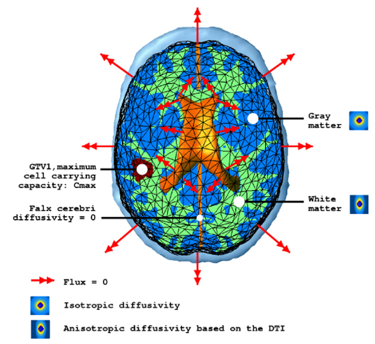
Diffusion model and boundary conditions summary.

Fig. 7.

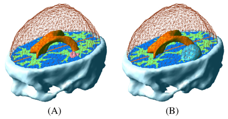
Tumor initialization in the finite element model. (A) GTV1. (B) GTV2.

Fig. 9.

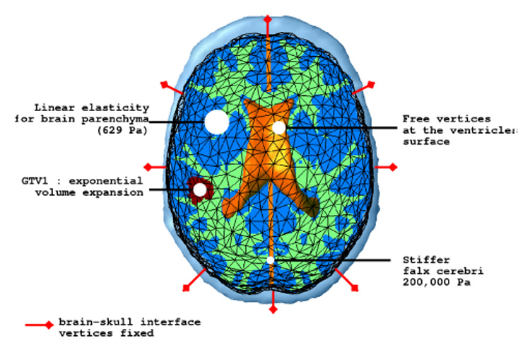
Mechanical model and boundary conditions summary.

The material diffusivity values are summed up in Table II. Figure 6 summarizes the diffusion model and the boundary conditions. The model is first used to solve the stationary version of Equation 11, so as to interpolate the c function between the two initial contours delineating the GTV1 and GTV2 (Figure 7).

TABLE II.

DIFFUSIVITY PROPERTY OF THE ATLAS SEGMENTED TISSUES

Tissue	diffusivity (10−3mm² s−1)
White matter	α · $\underset{¯}{\underset{¯}{D_w}}$ (anisotropic)
Gray matter	β · max($\underset{¯}{\underset{¯}{D_t}}$) (isotropic)
Ventricles	0 (isotropic)
Skull	0 (isotropic)
Falx cerebri	0 (isotropic)

D. Growth of the Tumor: Mechanical Model

1) Brain Constitutive Equation

One can find in the literature several rheological experiments performed on the brain tissue. Most relevant ones in this domain are certainly those conducted by Miller [29] and Miga et al. [30]. In particular, Miller has carried out several in-vivo experiments on pig brains. He suggests that brain tissue can be modeled with an homogeneous hyper-viscoelastic non-isotropic material.

We use the classical continuum mechanics formalism ([31] p.28) to describe the mechanical behavior of the brain parenchyma. Since the deformation is very slow, we propose to use the static equilibrium equation:

$$\mathit{\text{div}}(\underset{¯}{\underset{¯}{\sigma }})+\underset{¯}{f_{\mathit{\text{ext}}}}=0$$ (13)

with σ̳ the internal stress tensor (Pa, also known as the Cauchy stress tensor) and $\underset{¯}{f_{\mathit{\text{ext}}}}$ the external force applied on the model (N, also known as body forces).

Although brain tissue is a non-linear and viscoelastic material, the experiments of Miller indicated that the 1D stress-strain non-linear constitutive equation of the brain parenchyma can be approximated for very slow deformations (>> 50 sec) by:

$$\begin{array}{lll}\sigma \hfill & =\hfill & \frac{2}{{\gamma }^5}\left(1-g_1-g_2\right)\left(-1-\gamma +{\gamma }^3+{\gamma }^4\right)\hfill \\ \hfill & \hfill & *\left(\left(2C_{200}\right)\left(1-\gamma -{\gamma }^3+{\gamma }^4\right)+C_{100}{\gamma }^2\right)\hfill \end{array}$$

with:

• γ is related to the strain ε: ε = ln(γ).

• σ is the uni-axial stress.

• g₁ = 0.450, g₂ = 0.365

• C₁₀₀ = 263 Pa, C₂₀₀ = 491 Pa

Since the growing process is very slow in our case (>> 1 day), and the measured deformation in the parenchyma is in the small deformation range (≤ 5%), we propose to linearize this equation. We thus consider a linear relationship for both the constitutive equation and the strain computation:

$$\underset{¯}{\underset{¯}{\sigma }}=\underset{¯}{\underset{¯}{K}}\underset{¯}{\underset{¯}{\epsilon }}$$ (14)

$$\underset{¯}{\underset{¯}{\epsilon }}=\frac{1}{2}(\underset{¯}{\underset{¯}{▽u}}+{\underset{¯}{\underset{¯}{▽u}}}^T)$$ (15)

• K̳ is the elasticity tensor (Pa).

• ε̳ is the linearized Lagrange strain tensor expressed as a function of the displacement u̲ (no units).

By minimizing the squared stress error made with the linear elasticity approximation in the range of small compressions (ε ∈ [−0.1; 0.0]), we found an optimal Young modulus E = 694 Pa. The absolute stress error for this value is then below 4.2 Pa (cf Figure 8).

Fig. 8.

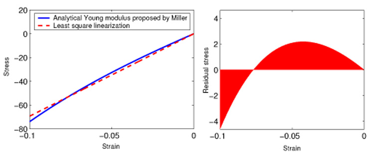
(Left) constitutive equation proposed by Miller and linear approximation; (right) stress error made with the linear approximation.

2) Mass Effect

We propose to make the difference between the mass effect induced by the GTV1 volume expansion and by the diffusion of tumor cells into the rest of the brain. We thus consider two distinct equations describing the mass effect.

a) Inside The GTV1

Because the GTV1 is modeled as a pure cell proliferation and since the associated tissue is considered as saturated with tumor cells, this proliferation directly acts as a volume increase on the GTV1. This volume increase ΔV can be computed at time t:

$$\Delta V=V_t-V_0=V_0(e^{\eta t}-1)$$

Based on the proposed model, η can be approximated by the average volume increase of GTV1 in GBM. We found η = 2.2 × 10⁻³ day⁻¹. However, because of the GTV1 inhomogeneity and because cells can be exchanged between the GTV1 and the GTV2, η does not directly characterize the GTV1 cells aggressiveness but represents an average volume expansion speed. As proposed in [32] we use a penalty method to impose this volume variation via a homogeneous pressure into the GTV1.

b) Outside The GTV1

Wasserman et al. proposed in [33] to model the mechanical expansion of the tumor volume by a pressure P proportional to N/V, with N the total tumor cell count and V the total volume of the tumor. We propose a new equilibrium equation to model the mechanical impact of the tumor on the invaded structures outside the GTV1.

$$\mathit{\text{div}}(\underset{¯}{\underset{¯}{\sigma }}-\lambda \underset{¯}{\underset{¯}{{𝕀}_3}}c)+\underset{¯}{f_{\text{ext}}}=0$$ (16)

This equation is the differential version of the law proposed in Wasserman et al. paper. It can be locally interpreted as a tissue internal pressure proportional to the tumor concentration.

3) Model Parameters and Initialization

The proposed mechanical model is similar to the one proposed to predict intra-operative deformations [34]. It has the following characteristics:

• a qualitative examination of the images did not show displacement between the brain and the skull, hence we assume that the brain does not slide on the skull. Since the skull is considered rigid, we fixed the brain mesh surface vertices. However, a brain-skull and a brain-falx cerebri sliding contact should be considered for patients showing a more significant mass effect, as proposed in [35], [29], [34].

• We use the linearized 3D homogeneous version of Miller’s constitutive equation (see III-D for details), the Young modulus is set to 694 Pa. One could also consider the additional anisotropy due to the white matter fibers. However without significant rheological experiments on this subject, we consider the brain tissue to be isotropic. We propose to model the brain parenchyma as almost incompressible, the Poisson coefficient is thus set to 0.40.

• Based on the intra-cranial flow model of Stevens [36], considering that the cerebro-spinal fluid production is not affected by the tumor growth, and because the growth process is very slow, we can consider that the ventricular pressure is not affected by the tumor growth. Therefore we let ventricular vertices free without additional internal pressure.

• The falx cerebri is a stiff fold of the dura-mater in the mid-sagittal plane and sustains part of the hemispheres internal pressure. We propose to stiffen the part of the mesh consisting of the falx. Based on the experimental results [37], we chose its Young modulus equal to 2 × 10⁵ Pa.

• We chose a coupling factor λ which minimizes the quantitative difference between the model and the real deformations: λ = 1.4 × 10⁻⁹ N mm Cells⁻¹. It corresponds to a 15% volume increase for a tissue with a saturated tumor cell density C_max.

The material mechanical properties are summarized in Table III. Figure 9 shows the mechanical model and the boundary conditions.

TABLE III.

MECHANICAL PROPERTIES OF THE DIFFERENT SEGMENTED TISSUES OR EQUIVALENT BOUNDARY CONDITIONS

Tissue	Young Modulus (Pa)	Poisson Coefficient
White	694	0.4
Gray Matter	694	0.4
Falx Cerebri	200,000	0.4
Ventricles	0	0
Skull	∞	0.5

E. Finite Element Method Discretization

We use the finite element method to discretize both problems. This numerical method suited for solving problems described by a partial differential equation (PDE) searches for solutions in a sub-vectorial space of finite dimension. The solution is thus expressed in the discretized domain by the shape functions and its associated nodal unknowns (more details about the general finite element framework can be found in [38]). Details of the FE modeling and numerical schemes are given in Appendices.

IV. RESULTS

After performing the simulation, we registered both the deformations and the tumor density to the first patient MRI (03/2001). Results are presented in two parts, the mass effect and the tumor invasion.

A. Mass Effect

Figure 10 shows the displacement of the brain parenchyma due to the mass effect. Even if the largest displacements occurs nearest the GTV1, distant tissues in the same hemisphere can be affected by the tumor growth. The average displacement at the GTV1-GTV2 boundary is about 3 mm. Figure 11 shows a close-up view on structure displacements induced by the mass effect. We can also observe that the tumor pushes the mid-sagittal plane away. The tumor has an influence on ventricle size: we measured a volume variation ΔV = 4.6 ml for the lateral ventricles for an initial volume of 25 ml. To quantify the accuracy of the simulation, a medical expert manually selected corresponding feature points³ on the patient MRIs so as to estimate these landmark displacements between March and September 2001. These measured displacements can then be compared to model-simulated ones. Table IV shows the result of this comparison. The average displacement for selected landmarks is 2.7 mm and the corresponding average error is 1.3 mm.

Fig. 10.

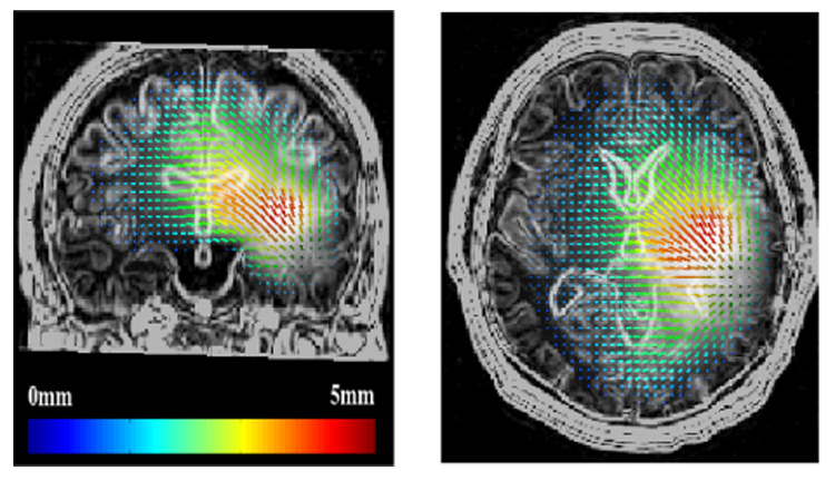
Displacement of the tissues induced by the tumor mass effect

Fig. 11.

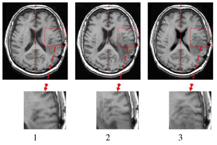
Visualization of the mass effect. 1. T1 MRI 03/2001, 2. T1 MRI 09/2001, 3. T1 MRI 03/2001 deformed with the simulated displacement field.

TABLE IV.

COMPARISON BETWEEN THE MEASURED (M̲) AND THE SIMULATED DISPLACEMENTS (S̲) ON SELECTED LANDMARKS. (ERROR NORM) = ‖M̲ - S̲‖. (NORM ERROR) = ‖M̲‖ - ‖S̲‖. (ANGULAR ERROR) = $\widehat{\underset{¯}{M}\underset{¯}{S}}$.

#	Measured displacement [x,y,z] norm (mm)	Simulated displacement [x,y,z] norm (mm)	Error norm (mm)	Norm error (mm)	Angular error °
1	[−3.0,1.0,1.0] 3.3	[−2.1,0.9,1.2] 2.6	0.9	0.7	11
2	[−1.0,−4.0,0.0] 4.1	[−0.8,−2.3,0.8] 2.7	1.8	1.4	18
3	[−1.3,−0.3,0.0] 1.3	[−1.3,−0.5,−0.1] 1.4	0.2	0.1	9
4	[−3.0,0.0,−0.6] 3.0	[−2.0,0.9,1.9] 2.9	2.9	0.1	56
5	[−2.3,−4.3,1.3] 5.0	[−1.7,−3.6,2.2] 4.7	1.2	0.3	14
6	[−0.6,0.0,−0.3] 0.7	[−1.5,0.5,0.3] 1.6	1.1	0.9	41
7	[−0.6,−1.0,−0.3] 1.2	[−0.3,−0.1,−0.2] 0.4	1.0	0.8	41

A second experiment was run without modeling the mechanical influence of the reaction-diffusion outside the GTV1 (modeled by Equation 16). We could thus evaluate the (mechanical) improvement added by the modeling of the reaction-diffusion component versus a simple volume expansion of the GTV1. Keeping the model unchanged (without modifying the pressure penalty constraint in the GTV1), the average error measured on landmarks is 80% higher (2.2 mm). This error remains 20% higher (1.6 mm) after optimizing the volume variation of the GTV1 to minimize the landmark error.

This experiment demonstrates the benefit of modeling the mechanical influence of the reaction-diffusion component. The remaining error on the mechanical coupling might be due to various phenomena:

• The ratio between the average deformation amplitude (2.7 mm) and the image resolution (1.0 mm) is not sufficient to make accurate measurements.

• The average error (1.3 mm) is in the range of manual selection error.

• The deformation might be more important in the sulci interstitial space than in the brain parenchyma. In such a case, a finer mesh and different constitutive equations would be necessary to model the deformation.

B. Reaction-Diffusion

Since we want to compare the simulation with the patient MRI, a correspondence between the c value and the MRI gray level needs to be established. Such a correspondence cannot however be found for two reasons:

• The hyper-signal observed in the T2 MRI does not directly correspond to the tumor but to the edema.

• Unlike CT, MRI is not a calibrated measure. Thus no absolute correspondence can be made between the gray level and the nature of the tissue.

Indeed, this correspondence has been measured on CT images. Tracqui et al. suggested a 8000 cells mm⁻³ threshold of detection in [14] for an enhanced CT scan. Figure 12 present the result of the GBM simulation above 8000 cells mm⁻³ on 8 different axial brain slices. These figures show a good agreement between the simulation and the data. The model manage to simulate complex tumor behaviors: for example, the ”Y” shape around the putamen observable on slices 3 and 4 of Figure 12 is recovered. Also, almost non-invaded tissues in March 03 could get a significant and realistic invasion 6 months later (slices 1,5).

Fig. 12.

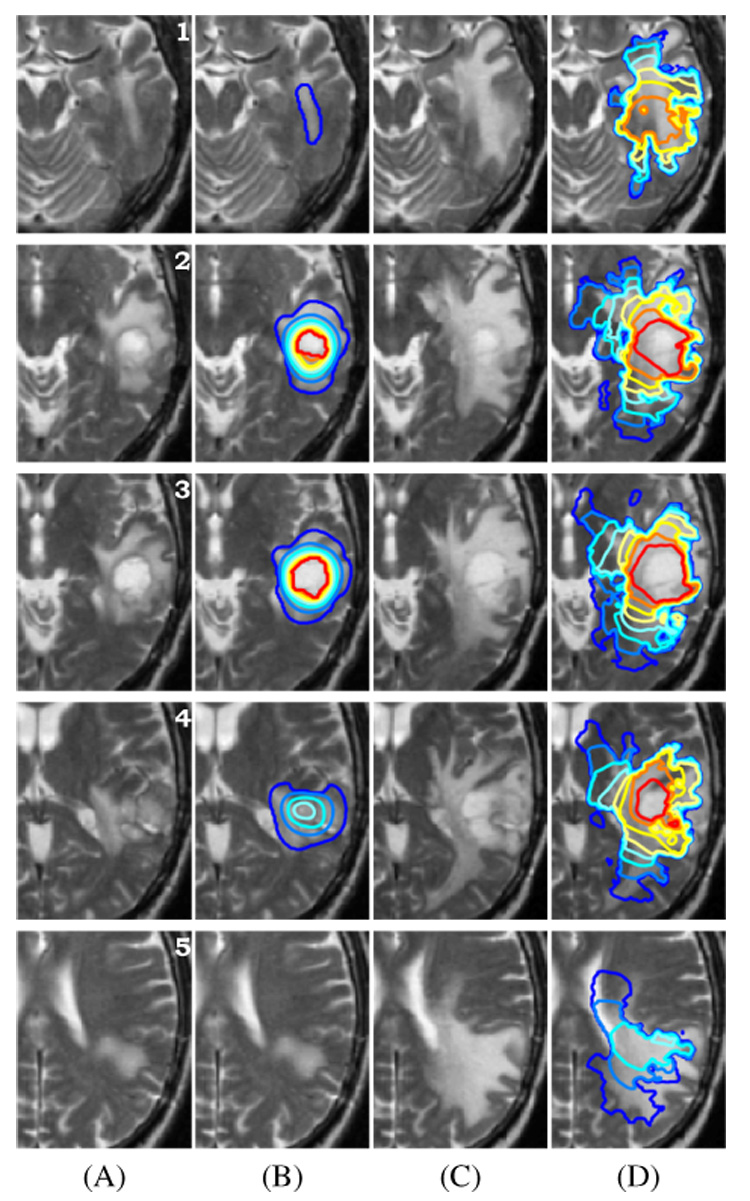
Result of the GBM growth simulation on slices # 1 → 5 of the brain. (A) MR T2 image of the patient in March 2003. (B) MR T2 image in March 2003 + superimposed simulation initialization contours. (C) MR T2 image of the patient in September 2003 (corresponding slice after rigid registration). (D) Contours of the 6 months tumor growth simulation above 8000 cells mm⁻³ superimposed on the MR T2 image in September 2003.

The simulation of the tumor-density evolution may be subject to different potential error sources:

• the segmentation based on an atlas matching method, may be improved using a more complex transformation (for example the non-linear registration method proposed in [39]).

• The registration of another subject DTI assumes that inter-subject variability on white matter distribution is limited, but this assumption and potential limitations need to be further studied.

• The adequacy of the reaction-diffusion equation to model the tumor invasion.

• Approximations made by the finite element method, and the error due to the discretization.

The influence of every factor will be part of our upcoming research.

V. PERSPECTIVES AND FUTURE WORK

We consider two distinct potential areas of research for the current model. One consists in improving the model for simulation, the other is related to the clinical validation and applications.

A. Model Improvement

Previous results have demonstrated the ability of the numerical model to predict the tumor invasion. However, the model could be enhanced with additional characteristics:

• When diffusing into the brain parenchyma, the tumor also affects the fibers of the white matter [40], [22]. This modification of the fiber structure in the invaded area could be taken into account by updating the diffusion tensor $\underset{¯}{\underset{¯}{D_t}}$.

• We could evaluate the adequacy of more complex diffusion laws, like the active cell model proposed by Tracqui et al. [11], to account for the growth of the GBM.

• The model could greatly benefit from the use of more patient-specific images. More precisely, patient DTI capturing the white-matter fiber directions could greatly improve the accuracy of the simulation.

• Using alternative numerical methods like finite differences on a structured grid could increase the resolution of the simulated tumor growth.

• Multi-scale models are important for improving therapies, and linking growth models at a cell and at a molecular scale with the reaction-diffusion equation remains our long-term goal.

B. Clinical Validation and Applications

Because this article describes a proof-of-concept aiming to demonstrate the feasibility of modeling complex tumors, we consider the comparison of the simulated tumor growth with the follow-up MR image of the patient as a preliminary step toward a clinical validation. In the future, we wish to develop methods dedicated to parameter identification and clinical validation, including:

• the correlation of the VG prediction with histo-pathological analysis of the patient’s brain, especially under the threshold of detection of the scanner.

• The inclusion of functional information to the atlas to allow the prediction of functional loss induced by the tumor growth.

• The study of the influence of the therapeutic intervention on the GBM invasion to better estimate the appropriate time for radiotherapy and surgery treatments, as proposed in [41].

We also wish to evaluate the relevance of the model on more patient datasets. This evaluation relies upon the influence of the initialization in the diffusion process, particularly in the GTV2. Finally, we wish to investigate the extension of the diffusive tumor model to other organs (lungs, muscles).

APPENDIX

a) Elements

We use a linear tetrahedron (P₁) element to discretize our brain domain (more details about the meshing procedure can be found in the next section). Then the displacement u of any point X̲ of the domain is defined as:

$$\underset{¯}{u}(\underset{¯}{X})={\displaystyle \sum _{j=0}^3{h}_j(\underset{¯}{X})\underset{¯}{u_j}}$$ (17)

And the cell density c:

$$c(\underset{¯}{X})={\displaystyle \sum _{j=0}^3{h}_j}(\underset{¯}{X})c_j$$ (18)

where h_j(X̲), j = 0,…,3 are the shape functions that correspond to the linear interpolation inside a tetrahedron and u_j is the displacement of vertex j of the tetrahedron. Using the homogeneous coordinates, the shape functions h_j(X̲) are related to the coordinates $\underset{¯}{{\mathrm{P}}_j}$ of a tetrahedron vertices by:

$$\begin{array}{lll}\underset{¯}{X}\hfill & =\hfill & \underset{¯}{\underset{¯}{P}}\underset{¯}{H}\hfill \\ \left[\begin{array}{c}x\\ y\\ z\\ 1\end{array}\right]\hfill & =\hfill & \left[\begin{array}{cccc}{p}_0^x& p_1^x& p_2^x& p_3^x\\ p_0^y& p_1^y& p_2^y& p_3^y\\ p_0^z& p_1^z& p_2^z& p_3^z\\ 1& 1& 1& 1\end{array}\right]\left[\begin{array}{c}{h}_0\\ h_1\\ h_2\\ h_3\end{array}\right]\hfill \end{array}$$ (19)

Note that the gradient $\underset{¯}{\underset{¯}{{▽}_u}}\left(\underset{¯}{X}\right)$ is constant inside the tetrahedra. More details about the computation of the shape function and its properties can be found in [42].

b) Mechanical Functional

The displacement field solution of the mechanical problem is obtained by minimizing the potential energy functional E_p:

$$E_p=\frac{1}{2}{\displaystyle {\int }_{\Omega }Tr[\underset{¯}{\underset{¯}{\epsilon }}\underset{¯}{\underset{¯}{K}}}\underset{¯}{\underset{¯}{\epsilon }}]d\Omega -{\displaystyle {\int }_{\Omega }\underset{¯}{f_{\text{ext}}}}\underset{¯}{U}d\Omega$$ (20)

Then combining Equations 17 and 15 with 20 we can explicitly compute the potential energy:

$$E_p=\frac{1}{2}{[u]}^T[K][u]-{[f]}^T[u]$$

The minimization condition can indeed be written as a linear system:

$$[K][u]=[f]$$ (21)

Details of the matrix [K] computation can be found in [42].

c) Diffusion Functional

Searching the solution of Equation 11 on a domain Ω (the brain) in a functional space ν (here ν = H¹) is equivalent to solving:

$$\forall \psi \in \nu ,{\displaystyle {\int }_{\Omega }\frac{\partial c}{\partial t}}·\psi ={\displaystyle {\int }_{\Omega }(\mathit{\text{div}}(\underset{¯}{\underset{¯}{D}}}\underset{¯}{▽c}))·\psi +{\displaystyle {\int }_{\Omega }\rho }c·\psi$$

Using the divergence theorem on the first term of the right side, and taking into account boundary conditions (details can be found in [38]), yields:

$$\forall \psi \in \nu ,{\displaystyle {\int }_{\Omega }\frac{\partial c}{\partial t}}·\psi =-{\displaystyle {\int }_{\Omega }\underset{¯}{\underset{¯}{D}}}\underset{¯}{▽c}·\underset{¯}{▽\psi }+{\displaystyle {\int }_{\Omega }\rho c·\psi }$$ (22)

Then combining 18 with 22 and taking ψ = h_j inside the tetrahedra, we can write the diffusion functional as:

$$\begin{array}{lll}{\displaystyle \sum _{i=1}^N\frac{\partial c_i}{\partial t}{{\displaystyle \int }}_{\mathrm{\Omega }}{h}_i{h}_j}\hfill & =\hfill & -{\displaystyle \sum _{i=1}^N{c}_i{{\displaystyle \int }}_{\mathrm{\Omega }}}\underset{¯}{\underset{¯}{D}}\underset{¯}{\nabla h_i}\cdot \underset{¯}{\nabla h_j}\hfill \\ \hfill & \hfill & +{\displaystyle \sum _{i=1}^N\left[c_i\right]}{{\displaystyle \int }}_{\mathrm{\Omega }}\rho h_i{h}_j\hfill \\ \hfill \left[M\right]\frac{\partial \left[c\right]}{\partial t}& =\hfill & \left(\rho \left[M\right]-\left[D\right]\right)\left[c\right]\hfill \end{array}$$ (23)

With the rigidity and mass matrices defined as:

$$\begin{array}{lllll}[M]\hfill & =\hfill & [M_{i,j}]\hfill & =\hfill & {\displaystyle {\int }_{\Omega }{h}_i{h}_j}\hfill \\ [D]\hfill & =\hfill & [D_{i,j}]\hfill & =\hfill & {\displaystyle {\int }_{\Omega }\underset{¯}{\underset{¯}{D}}}\underset{¯}{\nabla h_i}\cdot \underset{¯}{\nabla h_j}\hfill \end{array}$$

In addition, we perform mass lumping which consists in concentrating the mass of tetrahedra on their vertices. The mass matrix for tetrahedron T is then defined as:

$$[M_{i,j}]=0[M_{i,i}]={\displaystyle \sum _{T/(p_i\in T)}\frac{V(T)}{4}}$$

d) Mesh Generation

The full meshing procedure can be decomposed in three steps:

• Using the atlas segmented brain, a surface mesh is generated with the fast marching cube algorithm [43].

• This surface mesh is then decimated with the YAMS (INRIA) software [44].

• The volumetric mesh is finally generated from the surface one with another INRIA software: GHS3D [45]. This software optimizes the shape quality of all tetrahedra in the final mesh.

Since the structures considered in the segmentation (white matter fiber bundles, sulci) have a small size (between 1 and 4 mm), a fine mesh consisting of 250,000 tetrahedra has been used to mesh the brain.

e) Tetrahedra Labeling

In order to assign each tetrahedron its mechanical and diffusive properties from the five segmented classes in the atlas, the atlas-voxels contained in a tetrahedron have to be listed. We propose to ”slice” every tetrahedron, and include a voxel in a tetrahedron if its barycentric coordinates are positive. Analytically a voxel is assigned to the tetrahedron if:

$$\left\{\forall i\in \left[\mathrm{1..4}\right],{\left[{\underset{¯}{\underset{¯}{P}}}^{-1}\underset{¯}{X}\right]}_i>0\right\}$$

Each tetrahedron is finally classified according to the dominant voxel class in its volume. Based on this classification, the properties of the tetrahedra can be assigned according to Tables II and III.

f) Mechanical Equation

Numerical Integration: The linear system 21 can be written for each vertex i:

$$[K_{i,i}][u_i]+{\displaystyle \sum _{j\in N(i)}[K_{i,j}]}[u_j]=[f_i]$$ (24)

Where N(i) is the set of neighboring vertices of vertex i.

The principle of relaxation algorithms consists in moving each vertex in order to locally solve Equation 24 (see [46] for details):

$${[}^{+}{u}_i]={[K_{i,i}]}^{-1}[f_i]-{\displaystyle \sum _{j\in N(i)}{[K_{i,i}]}^{-1}[K_{i,j}][u_j]}$$ (25)

This method does not need the computation of a global stiffness matrix inverse, and could also be used for real-time simulation.

g) Reaction-Diffusion Equation

Numerical Integration: We propose an unconditionally stable implicit numerical scheme for the reaction-diffusion equation integration. Equation 23 thus becomes:

$$\begin{array}{lll}\left[M\right]\frac{{\left[c\right]}^{\tau +\mathrm{\Delta }\tau }-{\left[c\right]}^{\tau }}{\mathrm{\Delta }\tau }\hfill & +\hfill & \left[D\right]{\left[c\right]}^{\tau +\mathrm{\Delta }\tau }\hfill \\ \hfill & -\hfill & \rho \left[M\right]{\left[c\right]}^{\tau +\mathrm{\Delta }\tau }=0\hfill \end{array}$$

Which can be written as:

$$\left((1-\rho \mathrm{\Delta }\tau )+{[M]}^{-1}[D]\mathrm{\Delta }\tau \right){[c]}^{\tau +\mathrm{\Delta }\tau }={[c]}^{\tau }$$ (26)

In this way, Equation 23 is transformed into a linear system taking the form KU=F. The resolution method proposed for Equation 24 can then be used to solve the linear system 26.

REFERENCES

- 1.Haney S, Thompson P, Cloughesy T, Alger J, Toga A. Tracking tumor growth rates in patients with malignant gliomas: A test of two algorithms. American Journal of Neuroradiology. 2001 Jan;vol. 22(no. 1):73–82. [PMC free article] [PubMed] [Google Scholar]
- 2.Kantor G, Loiseau H, Vital A, Mazeron JJ. Gross tumor volume (gtv) and clinical target volume (ctv) in adult gliomas. Cancer Radiother. 2001 October;vol. 5(no. 5):571–580. doi: 10.1016/s1278-3218(01)00107-x. [DOI] [PubMed] [Google Scholar]
- 3.Retsky MW, Swartzendruber DE, Wardwell RH, Bame PD. Is gompertzian or exponential kinetics a valid description of individual human cancer growth? Med Hypotheses. 1990 October;vol. 33(no. 2):95–106. doi: 10.1016/0306-9877(90)90186-i. [DOI] [PubMed] [Google Scholar]
- 4.Lazareff JA, Suwinski R, De Rosa R, De RR, Olmstead CE. Tumor volume and growth kinetics in hypothalamic-chiasmatic pediatric low grade gliomas. Pediatr Neurosurg. 1999 June;vol. 30(no. 6):312–319. doi: 10.1159/000028817. [DOI] [PubMed] [Google Scholar]
- 5.Bajzer Z. Gompertzian growth as a self-similar and allometric process. Growth Dev Aging. 1999 Spring-Summer;vol. 63(no. 1–2):3–11. [PubMed] [Google Scholar]
- 6.Patel A, Gawlinski E, Lemieux S, Gatenby R. A cellular automaton model of early tumor growth and invasion. Journal of Theoretical Biology. 2001 Dec;vol. 213(no. 3):315–331. doi: 10.1006/jtbi.2001.2385. [DOI] [PubMed] [Google Scholar]
- 7.Bussemaker H, Deutsch A, Geigant E. Mean-field analysis of a dynamical phase transition in a cellular automaton model for collective motion. Phys. Rev. Lett. 1997;vol. 78:5018–5021. [Google Scholar]
- 8.Murray J. Mathematical Biology. New York: Springer-Verlag; 2002. [Google Scholar]
- 9.Swanson K, Alvord E, Jr, Murray J. Virtual brain tumours (gliomas) enhance the reality of medical imaging and highlight inadequacies of current therapy. British Journal of Cancer. 2002 Jan;vol. 86(no. 1):14–18. doi: 10.1038/sj.bjc.6600021. [DOI] [PMC free article] [PubMed] [Google Scholar]
- 10.Chaplain M. Avascular growth, angiogenesis and vascular growth in solid tumours: The mathematical modelling of the stages of tumour development. Mathematical and Computer Modelling. 1996;vol. 23(no. 6):47–88. [Google Scholar]
- 11.Tracqui P. From passive diffusion to active cellular migration in mathematical models of tumour invasion. Acta Biotheoretica. 1995 Dec;vol. 43(no. 4):443–464. doi: 10.1007/BF00713564. [DOI] [PubMed] [Google Scholar]
- 12.Zhou W-N, Chen Z-P, You C, Mu Y-G, Sai K, Zhang J-Y, Zhang X-H, Cheng J-J, Xu H-C. Individualized therapy and outcomes of microsurgery, radiotherapy, and chemotherapy for astrocytoma. Ai Zheng. 2004 November;vol. 23(no. 11) Suppl 1:1555–1560. [PubMed] [Google Scholar]
- 13.Burgess PK, Kulesa PM, Murray JD, Alvord ECJ. The interaction of growth rates and diffusion coefficients in a three-dimensional mathematical model of gliomas. J Neuropathol Exp Neurol. 1997 June;vol. 56(no. 6):704–713. [PubMed] [Google Scholar]
- 14.Tracqui P, Cruywagen G, Woodward D, Bartoo G, Murray J, Alvord E., Jr A mathematical model of glioma growth: the effect of chemotherapy on spatio-temporal growth. Cell Proliferation. 1995 Jan;vol. 28(no. 1):17–31. doi: 10.1111/j.1365-2184.1995.tb00036.x. [DOI] [PubMed] [Google Scholar]
- 15.Tracqui P, Mendjeli M. Modelling three-dimensional growth of brain tumours from time series of scans. Mathematical Models and Methods in Applied Sciences. 1999 June;vol. 19(no. 4):581–598. [Google Scholar]
- 16.Dawant BM, Hartmann SL, Pan S, Gadamsetty S. Brain atlas deformation in the presence of small and large space-occupying tumors. Comput Aided Surg. 2002;vol. 7(no. 1):1–10. doi: 10.1002/igs.10029. [DOI] [PubMed] [Google Scholar]
- 17.Frenay M, Lebrun C, Lonjon M, Bondiau PY, Chatel M. Upfront chemotherapy with fotemustine (f) / cisplatin (cddp) / etoposide (vp16) regimen in the treatment of 33 non-removable glioblastomas. Eur J Cancer. 2000 May;vol. 36(no. 8):1026–1031. doi: 10.1016/s0959-8049(00)00048-4. [DOI] [PubMed] [Google Scholar]
- 18.Ourselin S, Roche A, Prima S, Ayache N. Block matching: A general framework to improve robustness of rigid registration of medical images. In: DiGioia A, Delp S, editors. Third International Conference on Medical Robotics, Imaging And Computer Assisted Surgery (MICCAI 2000), ser. LNCS; october 11-14; Pittsburgh, Pennsylvanie USA: Springer; 2000. pp. 557–566. [Google Scholar]
- 19.Rousseeuw P. Least median-of-squares regression. Journal of the American Statistical Association. 1984;vol. 79:871–880. [Google Scholar]
- 20.Cocosco C, Kollokian V, Kwan R-S, Evans A. Brainweb: Online interface to a 3d mri simulated brain database. NeuroImage. 1997;vol. 5:425. [Google Scholar]
- 21.Bondiau P-Y, Malandain G, Chanalet S, Marcy P-Y, Habrand J-L, Fauchon F, Paquis P, Courdi A, Commowick O, Rutten I, Ayache N. Atlas-based automatic segmentation of mr images: validation study on the brainstem in radiotherapy context. Int J Radiat Oncol Biol Phys. 2005 January;vol. 61(no. 1):289–298. doi: 10.1016/j.ijrobp.2004.08.055. [DOI] [PubMed] [Google Scholar]
- 22.Price S, Burnet N, Donovan T, Green H, Pena A, Antoun N, Pickard J, Carpenter T, Gillard J. Diffusion tensor imaging of brain tumours at 3t: A potential tool for assessing white matter tract invasion? Clin Radiol. 2003 June;vol. 58(no. 6):455–462. doi: 10.1016/s0009-9260(03)00115-6. [DOI] [PubMed] [Google Scholar]
- 23.Sierra R. Nonrigid registration of diffusion tensor images, Master’s thesis. Swiss Federal Institute of Technology Zurich (ETHZ); 2001. Mar, [Google Scholar]
- 24.Alexander DC, Pierpaoli C, Basser PJ, Gee JC. Spatial transformations of diffusion tensor magnetic resonance images. IEEE Trans Med Imaging. 2001 November;vol. 20(no. 11):1131–1139. doi: 10.1109/42.963816. [DOI] [PubMed] [Google Scholar]
- 25.Xu D, Mori S, Shen D, van Zijl PC, Davatzikos C. Spatial normalization of diffusion tensor fields. Magn. Reson. Med. 2003 July;vol. 50(no. 1):175–182. doi: 10.1002/mrm.10489. [DOI] [PubMed] [Google Scholar]
- 26.Cruywagen G, Woodward D, Tracqui P, Bartoo G, Murray J, Alvord E. The modelling of diffusive tumours. Journal of Biological Systems. 1995;vol. 3(no. 4):937–945. [Google Scholar]
- 27.Swanson K, Alvord E, Jr, Murray J. A quantitative model for differential motility of gliomas in grey and white matter. Cell Proliferation. 2000 Oct;vol. 33(no. 5):317–329. doi: 10.1046/j.1365-2184.2000.00177.x. [DOI] [PMC free article] [PubMed] [Google Scholar]
- 28.Swanson K, Bridge C, Murray JD, Alvord EC. Virtual and real brain tumors: using mathematical modeling to quantify glioma growth and invasion. J Neurol Sci. 2003 Dec;vol. 216(no. 1):1–10. doi: 10.1016/j.jns.2003.06.001. [DOI] [PubMed] [Google Scholar]
- 29.Miller K. Biomechanics of Brain for Computer Integrated Surgery. Warsaw University of Technology Publishing House; 2002. [Google Scholar]
- 30.Miga M, Paulsen K, Kennedy F, Hoopes P, Hartov A, Roberts D. In vivo analysis of heterogeneous brain deformation computations for model-updated image guidance. Computer Methods in Biomechanics and Biomedical Engineering. 2000;vol. 3(no. 2):129–146. doi: 10.1080/10255840008915260. [DOI] [PubMed] [Google Scholar]
- 31.Fung Y-C. Biomechanics: Mechanical Properties of Living Tissues. Springer Verlag; 1993. [Google Scholar]
- 32.Kyriacou S, Davatzikos C. A biomechanical model of soft tissue deformation, with applications to non-rigid registration of brain images with tumor pathology. Medical Image Computing and Computer-Assisted Intervention. 2001;vol. 1496:531–538. [Google Scholar]
- 33.Wasserman R, Acharya R. A patient-specific in vivo tumor model. Mathematical Biosciences. 1996 Sep;vol. 136(no. 2):111–140. doi: 10.1016/0025-5564(96)00045-4. [DOI] [PubMed] [Google Scholar]
- 34.Clatz O, Delingette H, Bardinet E, Dormont D, Ayache N. Patient specific biomechanical model of the brain: Application to parkinson’s disease procedure. In: Ayache N, Delingette H, editors. International Symposium on Surgery Simulation and Soft Tissue Modeling (IS4TM’03), ser. LNCS; Juan-les-Pins, France: Springer-Verlag; 2003. pp. 321–331. [Google Scholar]
- 35.Miga MI, Paulsen KD, Kennedy FE, Hartov A, Roberts DW. Model-updated image-guided neurosurgery using the finite element method: Incorporation of the falx cerebri. Lec. Notes in Comp. Sci. for 2nd Int. Conf. on MICCAI. 1999;vol. 1679:900–909. doi: 10.1007/10704282_98. [DOI] [PMC free article] [PubMed] [Google Scholar]
- 36.Stevens S. Mean pressures and flows in the human intracranial system, determined by mathematical simulations of a steady-state infusion test. Neurological Research. 2000;vol. 22:809–814. doi: 10.1080/01616412.2000.11740757. [DOI] [PubMed] [Google Scholar]
- 37.Schill M, Schinkmann M, Bender H-J, Mnner R. Biomechanical simulation of the falx cerebri using the finite element method; 18. Annual International Conference, IEEE Engeneering in Medicine and Biology. S; 1996. [Google Scholar]
- 38.Bathe K. Finite Element Procedures in Engineering Analysis. Englewood Cliffs, N.J: Prentice-Hall; 1982. [Google Scholar]
- 39.Stefanescu R, Commowick O, Malandain G, Bondiau P-Y, Ayache N, Pennec X. Non-rigid atlas to subject registration with pathologies for conformal brain radiotherapy. In: Barillot C, Haynor D, Hellier P, editors. Proc. of the 7th Int. Conf on Medical Image Computing and Computer-Assisted Intervention - MICCAI 2004, ser. LNCS; Saint-Malo, France: Springer Verlag; 2004. Sep, pp. 704–711. [Google Scholar]
- 40.Price SJ, Pena A, Burnet NG, Jena R, Green HAL, Green H, Carpenter TA, Pickard JD, Gillard JH. Tissue signature characterisation of diffusion tensor abnormalities in cerebral gliomas. Eur Radiol. 2004 October;vol. 14(no. 10):1909–1917. doi: 10.1007/s00330-004-2381-6. [DOI] [PubMed] [Google Scholar]
- 41.Swanson KR, A EC, Jr, Murray JD. Dynamics of a model for brain tumors reveals a small window for therapeutic intervention. Discrete and Continuous Dynamical Systems. 2004;vol. 4(no. 1):289–295. [Google Scholar]
- 42.Delingette H, Ayache N. Soft tissue modeling for surgery simulation. In: Ayache N, editor. Computational Models for the Human Body, ser. Handbook of Numerical Analysis (Ed : Ph. Ciarlet) Elsevier; 2004. pp. 453–550. [Google Scholar]
- 43.Lorensen W, Cline H. Marching cubes: a high resolution 3d surface constructionalgorithm; Siggraph 87 Conference Proceedings, ser. Computer Graphics; 1987. Jul, pp. 163–170. [Google Scholar]
- 44.Frey PJ. Yams a fully automatic adaptive isotropic surface remeshing procedure. INRIA, Technical Report RT-0252. 2001 November
- 45.Frey PJ, George PL. Mesh Generation. Hermes Science Publications; 2000. [Google Scholar]
- 46.Saad Y. Iterative Methods for Sparse Linear Systems. Boston, MA: PWS Publishing; 1996. [Google Scholar]