Comparing the Characteristics of Gene Expression Profiles Derived by Univariate and Multivariate Classification Methods

Abstract

One application of gene expression arrays is to derive molecular profiles, i.e., sets of genes, which discriminate well between two classes of samples, for example between tumour types. Users are confronted with a multitude of classification methods of varying complexity that can be applied to this task. To help decide which method to use in a given situation, we compare important characteristics of a range of classification methods, including simple univariate filtering, penalised likelihood methods and the random forest.

Classification accuracy is an important characteristic, but the biological interpretability of molecular profiles is also important. This implies both parsimony and stability, in the sense that profiles should not vary much when there are slight changes in the training data. We perform a random resampling study to compare these characteristics between the methods and across a range of profile sizes. We measure stability by adopting the Jaccard index to assess the similarity of resampled molecular profiles.

We carry out a case study on five well-established cancer microarray data sets, for two of which we have the benefit of being able to validate the results in an independent data set. The study shows that those methods which produce parsimonious profiles generally result in better prediction accuracy than methods which don’t include variable selection. For very small profile sizes, the sparse penalised likelihood methods tend to result in more stable profiles than univariate filtering while maintaining similar predictive performance.

1 Introduction

Gene expression microarray technologies allow the study of the simultaneous mRNA expression of thousands of genes and their comparison between different samples and under varying conditions. Of special interest is the construction of gene expression profiles for classification, for example of tumours, or to predict pathological characteristics and clinical outcomes of complex diseases such as cancer. A wide variety of classification methods have been applied to this task (for an overview see Dudoit et al. 2002, Dupuy and Simon 2007) and biologists and clinicians are confronted with a multitude of methods of different complexities. Thus, it is a difficult task to decide which method is best in a given context.

To help with this decision, we here compare the most important characteristics of a range of classification methods, from simple univariate filtering to penalised likelihood methods and state-of-the-art machine learning algorithms. We restrict ourselves to the binary classification problem, but all methods can be generalised to situations where one wants to discriminate between more than two classes.

It is an additional complicating factor that often there are several potentially contrasting aims involved. One very important goal is to construct gene expression profiles which have a good prediction accuracy, i.e. which are able to classify new samples with a small misclassification error. An additional aim is that the expression profiles can be interpreted in biological terms and provide insight into the data structure (e.g. Dudoit et al. 2002, Somorjai et al. 2003, Díaz-Uriarte and Alvarez de Andrés 2006). This implies parsimony, that is that profiles should contain only a relatively small number of genes, which can then be followed up by literature searches and functional experiments to determine their role in the biological processes influencing the phenotype of interest. A third desirable property, that is also related to the interpretability of profiles, is their stability in the sense that the set of genes selected into the molecular profile and the associated predictive performance should not vary much when the set of samples used for training is altered slightly (e.g. Díaz-Uriarte and Alvarez de Andrés 2006).

A basic principle of statistical analysis is to provide measures of uncertainty for all estimates. This also applies to molecular profiles derived from microarray gene expression data (Michiels et al. 2005, Ein-Dor et al. 2005, Simon 2006). This means that the uncertainty of genes associated with their inclusion in the profile should be assessed as well as the probability for a particular profile to be selected relative to other possible solutions. Here we address this issue by estimating the instability in molecular profiles using a resampling setup, where the data are repeatedly randomly split into training and validation data and the molecular profiles associated with each of the splits are compared. A perfectly stable profile would contain the same genes for all training/validation splits. We propose to use the Jaccard similarity measure to assess how similar the profiles for all data splits are.

The assessment of uncertainty is particularly important for data coming from high-throughput technologies such as gene expression microarrays, because for these data sources a large amount of instability is expected for two reasons. Firstly, such data are associated with large technical and biological variation leading to low signal-to-noise ratio. And secondly, the data are high-dimensional and usually comprise many more variables (p) than samples (n), which introduces multi-collinearity in the input data matrix leading to instability in the estimation procedure. This is known as the “large p, small n” problem.

One way of solving this problem is by using a univariate filtering method to reduce the number of variables (e.g. Golub et al. 1999, Dudoit et al. 2002, van’t Veer et al. 2002). However, expression levels are often quite highly correlated between genes, because genes are co-regulated or act in the same biological pathways. Univariate approaches do not take the correlation structure into account, in contrast to multivariate methods. Multivariate approaches that are capable of handling p >> n data sets include penalised likelihood methods where a penalty term added to the log-likelihood function enforces unique parameter estimates. Here, we employ and compare the L₁- and L₂-penalties which correspond to the lasso (Tibshirani 1996) and ridge (Hoerl and Kennard 1970) logistic regression models, as well as the elastic net which combines both penalties (Zou and Hastie 2005). Another approach comes from the machine learning community, where ensemble methods have been used extensively. These methods build powerful classifiers from many weak simple classifiers. Here, we apply random forests as a representative from this class of methods, since they have been shown to perform very well in the context of microarray data, especially when the method is combined with an additional variable selection step (Breiman 2001, Díaz-Uriarte and Alvarez de Andrés 2006).

In the following section, the classification methods to derive molecular profiles are described, the resampling setup used to assess the stability of profiles is specified and measures for quantifying stability are characterised. The methods are applied to five publicly available microarray gene expression data sets which are introduced in Section 3; for two of these independent data are available for validation. The results are presented in Section 4 and the paper concludes with a discussion.

2 Methods

2.1 Classification methods

We compare several binary classification methods, and use the logistic regression model for all methods except the random forest:

$$\mathrm{logit}\left(p(Y=1\mid X)\right)=X\beta ,$$

where $X\in {\mathbb{R}}^{n\times p}$ is the matrix of gene expression values, $\beta \in {\mathbb{R}}^p$ denotes the vector of regression coefficients and Y ∈ {0, 1}ⁿ is the binary response vector.

For all methods the amount of shrinkage and thus the sizes of the molecular profiles and their prediction performances depend on tuning parameters. For the univariate method this is simply the number of genes p* chosen to be included in a profile, while for the penalised regression methods they are the penalty parameters for the L₁ and L₂ norms λ₁ and λ₂. Several parameters can be tuned for the random forest methods, the most important one being number of variables to be considered for node splits in the decision trees. However, Díaz-Uriarte and Alvarez de Andrés (2006) perform an extensive sensitivity analysis and come to the conclusion that the performance of random forests is quite insensitive to the choice of tuning parameter values, and we follow their suggestions for the choice of parameter values for microarray data analyses.

For most analyses the statistical computing package R (R Development Core Team 2006) was used, in particular the affy library for data pre-processing of the Affymetrix data sets and the glm library for univariate logistic regression analyses. The R library glmpath was used for the elastic net and the randomforest and varSelRF libraries for random forest without and with variable selection, respectively. Ridge and lasso regression analyses were carried out with the BBR software by Genkin et al. (2007).

2.1.1 Univariate filtering

Univariate filtering methods select a small number of gene variables based on univariate statistics assessing the potential of individual genes for class prediction. Here, we use the gene effects estimated by logistic regression models fitted for each gene variable separately plus optionally any clinical covariates. The p* “best” genes with the largest absolute effects $\mid \widehat{\beta }\mid ∕s.e.\left(\widehat{\beta }\right)$ (where $\widehat{\beta }$ is the regression coefficient estimate and $s.e.\left(\widehat{\beta }\right)$ its observed standard error) are selected and together they build the molecular profile. Since this molecular profile does not directly correspond to a statistical model for prediction, a second analysis step has to be undertaken where the selected genes are used in a binary classification method.

Nearest-centroid classification (NC)

The simple nearest-centroid classification rule has often been applied successfully to gene expression data (e.g. van’t Veer et al. 2002, Michiels et al. 2005). First, centroids, i.e. mean average profiles, are constructed for each class based on the training data available for the selected genes in the molecular profile. New samples are then assigned to the class whose centroid is closer to the sample based on a similarity (or distance) measure, here Pearson’s correlation r. That is, for two classes 0 and 1, a sample with gene expression profile x = (x₁, ..., x_p*) is assigned to class 1 iff

$$r(x,{\stackrel{‒}{x}}_1)>r(x,{\stackrel{‒}{x}}_0),$$ (1)

where x̄_k (k ∈ {0, 1}) is the mean expression vector (centroid) in the training samples of class k.

Diagonal linear discriminant analysis (DLDA)

Dudoit et al. (2002) compared various classification rules for the univariate filtering approach. They selected between 10 and 200 variables in several microarray data sets and found that simple classification methods generally outperformed more complex methods in this context. In particular, diagonal linear discriminant analysis was found to perform very well. DLDA is similar to the nearest-centroid method, except that here the sample variances are taken into account. Sample x = (x₁, ..., x_p*) is assigned to class 1 rather than class 0 iff

$$\sum _{i=1}^{p^{\ast }}\frac{{(x_i-{\stackrel{‒}{x}}_{1i})}^2}{s_i^2}<\sum _{i=1}^{p^{\ast }}\frac{{(x_i-{\stackrel{‒}{x}}_{0i})}^2}{s_i^2},$$ (2)

where $s_i^2$ is the i^th diagonal element of the pooled variance estimate of the diagonal covariance matrix Σ, which is assumed to be the same for both class populations.

2.1.2 Multivariate penalised regression

Ridge regression

The ridge estimator ${\widehat{\beta }}_2$ (Hoerl and Kennard 1970) is the penalised maximum likelihood solution of a regression problem, where a penalty term is imposed on the log-likelihood function ℓ(β) which is proportional to a tuning parameter λ₂ > 0. For logistic regression the log-likelihood is given as

$$\ell \left(\beta \right)=\log p(Y\mid X,\beta )=-\sum _{j=1}^n\log (1+\exp (-Y_j{X}_j^T\beta )).$$ (3)

The penalty term contains the sum of squared regression coefficients ${\sum }_{i=1}^p{\beta }_i^2$ (i.e. the L₂ norm of β), so that the ridge regression estimator for a fixed penalty parameter λ₂ is given as

$${\widehat{\beta }}_2=\arg \underset{\beta }{\max }\left(\ell \left(\beta \right)-{\lambda }_2\sum _{i=1}^p{\beta }_i^2\right).$$ (4)

Finding the ridge regression solution is equivalent to determining the maximum a posteriori (MAP) estimate of the Bayesian regression model with independent and identical Gaussian priors β_i ∼ N(0, τ₂ > 0) on each parameter β_i, where the prior variance τ₂ is related to the penalty parameter λ₂ by τ₂ = 1/(2λ₂).

Lasso regression

Lasso regression (Tibshirani 1996) is similar to ridge regression, with the only difference being that here the L₁ norm of the regression coefficient vector ${\lambda }_1{\mid \mid \beta \mid \mid }_1={\lambda }_1{\sum }_{i=1}^p\mid {\beta }_i\mid$ is used, instead of the L₂ norm, leading to the optimisation problem

$${\widehat{\beta }}_1=\arg \underset{\beta }{\max }\left(\ell \left(\beta \right)-{\lambda }_1\sum _{i=1}^p\mid {\beta }_i\mid \right)$$ (5)

The penalised likelihood solution with the L₁ norm corresponds to the MAP estimate for the Bayesian regression model with independent, identical Laplace (also called double exponential) distributions with mean 0 and variance ${\tau }_1=2∕{\lambda }_1^2$ as priors on the β parameters.

Elastic net (ENet)

The naïve elastic net simply uses both L₁ and L₂ penalty terms in the penalised log-likelihood function:

$${\widehat{\beta }}_{12}=\arg \underset{\beta }{\max }\left(\ell \left(\beta \right)-{\lambda }_1\sum _{i=1}^p\mid {\beta }_i\mid -{\lambda }_2\sum _{i=1}^p{\beta }_i^2\right)$$ (6)

However, this results in over-shrinkage when compared to the lasso (Zou and Hastie 2005), and the estimates for β from the naïve elastic net are scaled to determine the final elastic net estimates:

$${\widehat{\beta }}_{EN}=(1+{\lambda }_2){\widehat{\beta }}_{12}.$$ (7)

The L₁-penalty has the advantage of automated variable selection over the L₂-penalty. This implies that for the lasso and the elastic net, the estimated effect of most variables will be shrunk to zero, effectively excluding them from the set of relevant covariates. Note that for the lasso method there is a practical restriction on the maximum number of variables which can be selected, which depends on the sample size n and number of variables p: min(n − 1, p) (Zou and Hastie 2005). This restriction does not apply to the elastic net.

All the estimated penalised regression models can be directly used for class prediction, since the logistic regression model provides probability estimates for class membership. A sample is predicted as belonging to a class, if the estimated class probability is larger than 1/2.

2.1.3 Random forest (RF) and varSelRF

The random forest classifier (Breiman 2001) is an example of the class of ensemble classification algorithms, which combine the outputs of many “weak” classifiers, in this case classification trees, to produce a powerful ensemble. The random forest can be successful in dealing with the multi-collinearity of “large p, small n” applications, because it combines two ideas to help find as many of the multiple best solutions as possible: firstly, it uses repeated bootstraps, that is each tree is grown using a different bootstrap sample of the data, and secondly it also employs random subspace selection, i.e. it only uses a random subset of all available variables to grow each tree. Because of this, for p >> n data it is likely that most or all variables will get used in node splits for some of the trees. The final classification is the mode of the classifications of all trees: the random forest chooses the class that has been decided by the majority of trees.

While random forests can deal with p >> n data, it has been found that the classification performance can be improved if the classifier is combined with a variable selection step so that only a small number of variables get used in the entire forest, see Díaz-Uriarte and Alvarez de Andrés (2006). There, the performance of random forests is compared to the varSelRF method, which implements variable selection by iteratively fitting random forests and discarding the variables which get used as nodes least often.

2.2 Multiple random validation study setup

We employ a multiple random validation setup (e.g. Michiels et al. 2005), where the data are repeatedly randomly divided into training data and validation data. We perform 50 random samplings, each with a ratio of 2:1 for the size of training to validation sample sizes. The resampling scheme is outlined in Table 1.

Table 1.

Resampling study setup for comparison of the characteristics of the classification methods

For k = 1, ..., m (m = 50): Divide data randomly, assigning 2/3 of the samples into a training set k and the remaining 1/3 into a validation set k (optionally, fix class proportions). For all classification methods, and for a set choice of tuning parameter values, fit classification model using training data set k and find molecular profile k. Apply fitted model to validation data k and assess prediction performance in terms of percentage of misclassified validation samples

2.3 Assessing the instability of molecular profiles

We view stability of gene expression profiles in terms of whether the same genes get selected for different training data sets. Naturally, this concept does not apply to those classifiers that use all the gene variables. Hence, we only assess the stability for those methods that do incorporate feature selection.

In the microarray literature most attempts to evaluate the stability of gene expression profiles for classification have focussed on resampling setups such as bootstrapping (Díaz-Uriarte and Alvarez de Andrés 2006) or repeated splits into training and validation subsets (Michiels et al. 2005). Examples include the approach taken by Díaz-Uriarte and Alvarez de Andrés (2006), Davis et al. (2006), Ma et al. (2006) and others, who argue that if gene sets are stable then the majority of genes will be included in most sets. Consequently, they use the inclusion frequencies to derive a single measure of stability, e.g. by averaging over the frequencies of all genes that get included at least once.

Another approach is to use the size of the intersection between gene sets. For example, Ein-Dor et al. (2005) consider all $\left(\begin{array}{c}\hfill m\hfill \\ \hfill 2\hfill \end{array}\right)$ pairwise comparisons between any two of the m = 50 gene sets and use the average of the sizes of the pairwise intersections as a single summary measure. Michiels et al. (2005) and Davis et al. (2006) use a generalisation of the joint intersection between all m gene sets, by considering the proportion of genes that get selected into > 50% or > 75% of all m profiles. Note that these approaches do not take the relative sizes of the gene sets into account, so that one cannot compare the stability of a classifier that produces large profiles with one producing very small profiles.

To reflect this, Blangiardo and Richardson (2007) propose the ratio of observed to expected size of intersection in a situation where gene sets are independent. However, in our resampling setup the gene sets are not independent since the various training subsets partly overlap, and in the absence of independence the expected size of intersection is difficult to obtain without computationally demanding data-dependent permutation studies.

In addition, relying on the size of the intersection between sets as a measure of similarity between the sets is not satisfactory in itself, because the intersection size does not fulfill several criteria (outlined in the next section) that are desirable in this context.

2.3.1 Similarity indices

There is a wide variety of similarity measures available for the comparison of sets (see Simpson 1960, Hazel 1970, Sokal and Sneath 1973, and others). Measures ρ(Z¹, Z²) for the comparison of two discrete sets Z¹ and Z² are usually based on the two-by-two table counting the presences and absences in both sets (Table 2).

Table 2.

2 × 2 table counting presences (1) and absences (0) in gene sets Z¹ and Z²

	Z1  1 0
Z2 1  0	a b c d

Generally, the gene expression profiles will be parsimonious, so that the number of present genes will be much smaller than the number of absent genes. Because of this we consider the presence of a gene in two profiles to contribute more to the similarity of these profiles than its absence and prefer measures which are independent of the value of d. In addition, the measure should also have a number of other desirable properties (e.g. Janson and Vegelius 1981, Sepkoski Jr. 1974), in particular

• symmetry: ρ(Z¹, Z²) = ρ(Z², Z¹),

• homogeneity: ρ(Z¹, Z²) does not change if the numbers a, b, and c are multiplied by the same constant, and

• boundedness: min(ρ(Z¹, Z²)) = 0 and max(ρ(Z¹, Z²)) = 1, and ρ(Z¹, Z²) = 0 ⇔ a = 0, ρ(Z¹, Z²) = 1 ⇔ b = c = 0.

Note that the simple intersection size a, which seems an obvious choice and has been proposed often (see the previous section), does not fulfill the homogeneity and boundedness criteria. This means that one cannot compare the values of a(Z¹, Z²) and a(Z³, Z⁴) computed for different pairs of sets, especially if the sets are of different sizes and hence the maximum possible value of a is different for both cases. Three popular measures that do fulfill the requirements and are better suited for comparisons are:

• Jaccard’s index (Jaccard 1901) ${\rho }_j(Z^1,Z^2)=\frac{a}{a+b+c}=\frac{\#(Z^1\cap Z^2)}{\#(Z^1\cup Z^2)}$

• Dice-Sorensen’s index (Dice 1945) ${\rho }_d(Z^1,Z^2)=\frac{2a}{a+b+c}$

• Ochiai’s index (Ochiai 1957) ${\rho }_o(Z^1,Z^2)=\frac{2a}{\sqrt{a+b}\sqrt{a+c}}$.

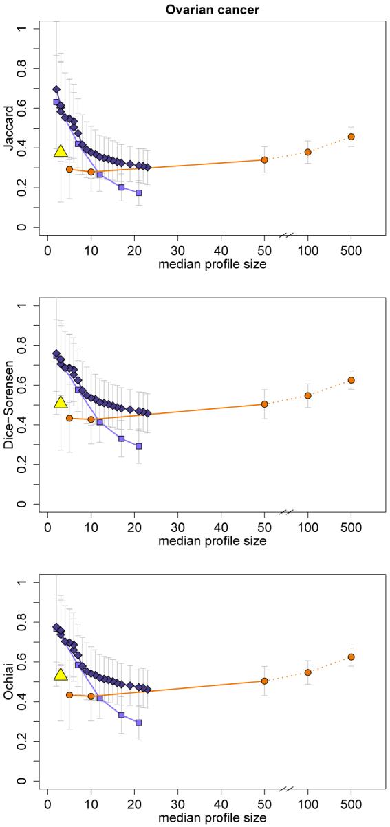
The Jaccard index is the ratio of set intersection size to set union size, which makes it intuitive and easy to interpret. The Dice-Sorensen and Ochiai indices can be interpreted as the harmonic and geometric means of the ratios a/(a+b) and a/(a + c), respectively. The Dice-Sorensen and Jaccard indices are very similar and in fact are increasing functions of each other with ρ_d = 2ρ_j/(1 + ρ_j) and ρ_j = ρ_d/(2 − ρ_d), so that for the purpose of comparison of different similarity values the two indices are equivalent. In our applications we found the harmonic mean index (Dice-Sorensen) and geometric mean index (Ochiai) to be very similar (see Figure 5 in Appendix A for one data set). Hence, throughout the paper we only show the results for the Jaccard index as a representative of the three similarity indices because it is arguably the most popular of the three measures.

The indices assess the similarity between pairs of sets, so in order to compare m > 2 sets we compute the indices of all possible $\left(\begin{array}{c}\hfill m\hfill \\ \hfill 2\hfill \end{array}\right)$ combinations of pairs of sets and assess the empirical distributions of these values.

3 Data

We apply the resampling scheme and assess the predictive accuracy and stability of the molecular profiles derived from the methods described in the previous section to five publicly available gene expression data sets, which are summarised in Table 3. In the resampling scheme, the samples are assigned randomly to either training or validation subset without restriction. An exception is the ovarian cancer data set, where only 17% of all samples belong to the less frequent class. Here, to ensure that all subsets contain samples from both classes, the class proportions in all training and validation subsets are fixed to be the same as in the complete data.

Table 3.

Main characteristics of gene expression microarray data sets used. Data sets in italics and brackets are used as validation data

	p	n	Response (binary)	Chip type
Ovarian cancer - Schwartz et al. (2002) (Lu et al. 2004)	7129 12625	104 42	tumour type (mucinous/clear-cell vs. endometrioid/serous)	HuGeneFL U95Av2
Leukaemia (ALL/AML) - Golub et al. (1999)	7129	72	tumour type (ALL vs. AML)	HuGeneFL
Prostate cancer - Singh et al. (2002)	12625	102	tumour vs. normal	U95Av2
Breast cancer - van’t Veer et al. (2002) (van de Vijver et al. 2002)	4770 4770	97 87	metastasis-free survival (≤ 5 yrs vs. > 5 yrs)	Agilent Agilent
Acute myeloid leukaemia (AML/karyotype) - Valk et al. (2004)	22283	273	normal vs. abnormal karyotype	U133A

In addition, for two of the data sets (breast and ovarian cancer) independent validation data sets are available. The breast cancer validation data (van de Vijver et al. 2002) have been generated by the same centre using the same platform and protocols as in the original study by van’t Veer et al. (2002). We only include samples in the validation set that were not part of the original study. In addition, we restrict our validation samples to lymph-node negative patients only, since that was an inclusion criterion for the original study.

In the instance of the ovarian cancer validation data the validation samples have been collected and processed by a different team in a study conducted independently from the original study by Schwartz et al. (2002). However, both study groups have very similar clinical characteristics and outcome data (Lu et al. 2004) and it is reasonable to assume that both groups come from comparable populations.

All gene expression data were generated using Affymetrix oligoarrays (although with several different chip types), except the breast cancer expression data, which were generated with Agilent two-colour arrays. All Affymetrix data are pre-processed and normalised in the same way using RMA background-correction (Irizarry et al. 2003) and loess regression for array normalisation (Cleveland 1979). An exception is the ALL/AML data set where the pre-processed data provided by the R package golubEsets were used.

All Affymetrix data are centered and scaled to zero mean and unit variance for all gene variables in the binary classification analysis. The Agilent data are normalised in the same way as described in the original paper (van’t Veer et al. 2002). After filtering and removing the small proportion of genes with missing values, 4770 genes remain for analysis.

Note that for the breast cancer data set, clinical data, which are known predictive factors for breast cancer progression, are available in addition to the gene expression data. These are patient age, tumour grade, tumour diameter and angioinvasion. Since the interest is in developing molecular profiles which can improve on predictive accuracy on top of known clinical factors, the clinical data are included in all classification methods and their effects are not allowed to be shrunken by the penalised likelihood methods nor to be removed from the active variable set in all other methods.

4 Results

Each of the five data sets is randomly split into training and validation subset m = 50 times. For each of the data sets all classification methods are fitted to each of the 50 training subsets for a range of tuning parameter values.

The tuning parameter values are carefully chosen to cover a wide range of models and model sizes. For univariate filtering the number of variables to be selected is p* ∈ {5, 10, 50, 100, 500}, since we assume that the inclusion of more than 500 gene variables will not result in further improvement of the predictive accuracy. For the Affymetrix data sets the ridge and lasso penalty parameters were chosen so that the corresponding prior variances τ range from 0.01 to 100 for lasso and from 10⁻⁵ to 1 for ridge regression (both on the log₁₀ scale). For lasso regression, the smallest profiles with τ = 0.01 usually contain less than 5 genes (an exception is the AML/karyotype data set). Since the data are normalised to have unit variance, the choice τ = 100 reflects an extremely large prior variance compared to the sample variances and induces very little shrinkage. Recall that in ridge regression no sparsity is induced, and hence the profile sizes cannot be used to determine the range of values for the penalty parameter. Instead, preliminary test runs were performed to ensure that the range of models with best prediction accuracy is covered for all data sets. Since the Agilent data are pre-processed and normalised in a different way to the Affimetrix data, slightly different penalty parameter values had to be chosen to cover the entire range of models (τ₁ ∈ {10⁻³, 10^−2.5, 10⁻², 10^−1.5, 10⁻¹} for lasso and τ₂ ∈ {10⁻⁶, 10⁻⁵, 10⁻⁴, 10⁻³, 10⁻²} for ridge). Note that for the elastic net two tuning parameters exist, which regulate the size of the L₁- and L₂-penalty terms, respectively. Here, we use a fixed penalty for the L₂-term (λ₂ = 1) and vary the size of the L₁-penalty parameter λ₁ from zero, resulting in the largest possible profiles, which are of comparable sizes to the largest observed lasso profiles, to a value large enough to induce maximum sparsity, i.e. so that no genes are included in the model.

4.1 Prediction accuracy

The fitted models can be applied to the corresponding validation subsets, where we record the proportion of misclassified samples as a measure of prediction accuracy, resulting in 50 misclassification error values per data set and fitted model, which are summarised as boxplots in Figure 1. We focus on the median values as the main measure for comparisons between methods. Note that for the elastic net (ENet) the misclassification rates can be quite large for very small molecular profiles, i.e. where the largest penalties are applied, but they quickly decrease and level off when the penalty is decreased and more genes are allowed to enter the model. For all of the data sets except the ALL/AML data, for univariate filtering (NC and DLDA) the misclassification rates decrease first but then rise again when increasing the profile size p*, especially when applying diagonal linear discriminant analysis (DLDA).

Figure 1.

Boxplots of predictive performances in terms of proportion of misclassified validation samples shown for a range of tuning parameter values. The median profile sizes (averaging across the 50 resampling sets) corresponding to each parameter value are indicated for all methods below the corresponding boxplots. The orange lines represent the baseline classification rates, where all samples are assigned to the most frequent class.

Note that because we want to compare characteristics of molecular profiles of different sizes, we do not tune the classification methods to optimise their performances in terms of minimal misclassification errors, i.e. we do not attempt to choose “optimal” tuning parameter values among those values presented alongside each other in Figure 1. Because of this there is no need to include an internal cross-validation or bootstrapping step within each of the m = 50 training/validation splits of the data. This would be necessary for an unbiased estimation of the generalisation error in order to avoid over-fitting when tuning parameters of classification methods.

The predictive accuracies that can be achieved by gene expression profiles vary widely between data sets. The first three data sets (ovarian cancer, ALL/AML, and prostate cancer) are easily separable, and the minimum median error rates correspond to as little as only one or two misclassified samples for the ovarian and prostate cancer data. Classification is not so easy for the last two data sets (breast cancer and AML/karyotype), where the best median error rates achieved are about 30%. This reflects the idea that different types of outcome data are more or less related to gene expressions. For example, tissue or tumour type can be explained to a large degree by gene expression, as we observe for the first three data sets. On the other hand, making a prognosis for cancer survival is a much more complex problem which is influenced to a large degree by environmental factors, as well as additional genetic factors other than just gene expression levels. This is in part reflected by the fact that for our breast cancer data, where clinical covariates are available, the use of these clinical variables alone for classification between patients with favourable and unfavourable survival prognosis already achieves a median misclassification proportion of 39%. So the additional inclusion of gene expression data as predictors only reduces the median error rate from 39% to about 30%.

In general, prediction performances of the lasso, elastic net, and univariate filtering methods all seem to be comparable in the sense that for all data sets we observe similar minimum values of the median error rates between these methods. There is not much difference between the two sparse penalised likelihood methods (lasso and elastic net); the additional L₂-penalty term introduced in the elastic net does not seem to improve the prediction accuracy. Remember that the two univariate filtering methods only differ in the final classifier applied to the selected genes; the gene lists themselves are identical. Despite this, the prediction performances can somewhat differ. In particular, DLDA achieves smaller median error rates than the nearest centroid (NC) methods for the prostate cancer and AML/karyotype data.

For the classification methods that do not perform automatic variable selection, i.e. ridge regression and the random forest (RF), the prediction performances are comparable to the other methods for some data sets (with equal or slightly larger median error rates), but in some cases they perform substantially worse. For example, both ridge regression and random forest have higher misclassification errors in the ovarian and breast cancer data, and in addition the random forest has higher error rates when applied to the prostate cancer data. The varSelRF method (random forest with variable selection) tends to have smaller prediction errors than the random forest without variable selection, except in the ALL/AML data set.

4.2 Ranking genes by their profile inclusion frequencies

Classification methods with inherent variable selection produce parsimonious gene expression profiles consisting of a small number of genes. In our case these methods are univariate filtering, lasso, elastic net and varSelRF. Since for these methods not all genes are selected into all profiles corresponding to the resampled training data subsets, we can rank the genes by their frequency of selection, giving a measure for the relative importance of a gene for class prediction (e.g. Michiels et al. 2005, Díaz-Uriarte and Alvarez de Andrés 2006). We will be more certain that a gene is relevant if it is selected most of the time. As an example, the selection frequencies are shown for the ovarian cancer data in Figure 2, for those genes which get selected into at least half of the profiles with any of the methods that incorporate variable selection (for at least one tuning parameter value). The selection frequencies for the different tuning parameter values are displayed as T-bars on top of each other, which become darker colours of gray with decreasing average profile sizes. For univariate filtering only the smaller profiles of sizes p* ∈ {5, 10, 50} are shown to avoid plot overcrowding.

Figure 2.

Inclusion frequencies for genes selected into at least half of all profiles by any of the methods for at least one tuning parameter value (ovarian cancer data). Frequencies corresponding to each of the parameter values are illustrated by overlaid T-bars varying from light gray for the largest profiles to black for the smallest. For example, the bar enclosed by the orange box shows gene X03635 being selected in all 50 univariate profiles of size p* = 50 (light gray), in 47 profiles with p* = 10 (darker gray) and in 43 with p* = 5 (black).

Lasso regression always selects the same five genes into more than half of the m = 50 resamples, for all penalty values λ₁ > 0.01. The same five genes also get chosen very often into elastic net profiles. Two of these (M82809 and U11862) are the only genes that get selected into more than half of the varSelRF profiles, which are generally very small with a median profile size of three. While we observe this good agreement for the multivariate methods, different genes are included most frequently by univariate filtering. Only one of the five genes always found by lasso is also part of more than half of the univariate profiles with p* ≤ 50 genes (X65614). This is reflective of the fact that variables get selected independently in the univariate filtering approach, while multivariate methods take into account the correlation structure between genes. Note that when the profile sizes become larger either by increasing p* or by decreasing the penalty parameter λ₁, genes that had been included often in smaller profiles, are generally included in the larger profiles as well and rarely get dropped.

4.3 Profile stability

In addition to assessing the frequencies of individual genes, we can use the resampling setup to evaluate the molecular profiles as a whole in terms of their stability. We compute the Jaccard similarity indices for all pairs of non-empty gene sets, which are summarised in Figure 3 by their means and standard deviation bars. The similarity values are plotted against the median gene set sizes to show how the stabilities of profiles constructed by the different classification methods develop with increasing profile sizes (which are induced by changing the tuning parameter values).

Figure 3.

Mean Jaccard similarity measures (± standard deviation) plotted against median profile sizes for univariate filtering, lasso regression, elastic net, and random forest with variable selection (varSelRF) for the five data sets and the ovarian cancer data with randomised response (top right).

In general, the observed Jaccard index distributions of elastic net and lasso are similar. The mean Jaccard values are largest for the smallest profiles which contain less than about ten genes. They then decline roughly monotonically with decreasing values of the penalty parameter λ₁ (which is equivalent to increasing profile sizes). The similarity values observed for the molecular profiles from univariate filtering follow a different pattern. They vary less across profile sizes and are largest for the very large profiles containing 100 or 500 genes, with the exception of the AML/karyotype data.

Note that this increase in similarity for very large univariate profiles can at least in part be explained by a spurious effect due to how the resampling study is designed. Because each of the m = 50 training subsets consists of two-thirds of the complete data sets, the expected intersection between any two training subsets is considerable: 4/9. Because of the overlap in samples, one expects a certain size of intersection between any two selected gene lists, even in cases where the gene expression data have no predictive power for the response of interest at all, for example because the response data have been randomised. This overlap can hence not be attributed to the classification method’s ability to produce stable profiles for classification.

This is illustrated in the top-right plot of Figure 3, where the classification analyses have been repeated for the ovarian cancer data set with the response variable having been randomised. Here, for small molecular profiles containing up to about 50 genes, the average similarity values between any two profiles are small (mean values ≤ 0.1) relative to the similarities observed for the non-randomised response data (top left in Figure 3). But for the largest profiles with 500 genes the mean similarity value increases to about 0.2, and so most of the increase in the original ovarian cancer data without randomised response, that is observed between the univariate profiles with p* = 50 and p* = 500, can be attributed to this effect. This analysis has been repeated with the other data sets as well and the same effect could always be seen. Hence, this effect needs to be accounted for when comparing similarity between different classification methods and across varying profile sizes, especially when very large profiles are involved. However, we found earlier that the best-performing methods in terms of prediction accuracy induce sparsity and profiles usually contain less than 50 genes on average. And for these profiles the effect is small and very similar across methods, posing no big problem.

Among the very parsimonious profiles (≤ 5 genes), lasso and elastic net molecular profiles tend to be equally or more stable than the univariate profiles with respect to our stability measures. An exception is the AML/karyotype data set where the univariate method has much larger similarity values across all profile sizes than all other methods. The random forest with variable selection is comparable to the penalised likelihood methods. For some applications, the computed similarity indices are very small for all but the smallest profiles, this applies in particular to the breast cancer data for all methods and to the AML/karyotype data for the penalised likelihood methods. After accounting for the effect of the resampling study design described above, the remaining stability that can be attributed to the classification method itself is even smaller.

We find that the overall stability patterns across the range of tuning parameter values are quite different between data sets. In particular, the similarities between profiles from univariate filtering vary widely. The profiles are least stable for the breast cancer data and most stable for the prostate cancer data. These differences in similarity distributions must be due to the differences in data structure, for example in the correlation structure between genes which are related to the response and get selected into classification profiles. Hence, for each profile we compute all pairwise correlations between all genes in the profile and record the mean of the absolute values of these correlations as a summary measure for the strength of correlations in that profile. The distributions of these mean absolute correlations across all m = 50 resamples are illustrated by their mean and standard deviations in Figure 4. As we observed for the Jaccard index, the relative sizes of these correlations differ between data sets, with the largest differences again being seen for univariate filtering methods. For all methods, the average correlations are largest for small profile sizes. However when profile sizes increase, the within-profile correlations decrease much faster for the multivariate methods than for univariate filtering.

Figure 4.

Distributions of means of absolute correlations within profiles (mean ± standard deviation) plotted against median profile sizes.

Note that the shapes of the median absolute correlations plotted against median profile sizes in Figure 4 closely resemble the shapes of median Jaccard similarities against median profile sizes in Figure 3. This suggests that the differences in similarity distributions between data sets might indeed be explained by differences in the correlation structures. It also means that whenever the averaged pairwise Jaccard similarities are large, i.e. when mostly the same genes get selected into the profiles, the absolute correlations between these genes tend to be large as well.

One big difference between univariate filtering and multivariate classification methods is that univariate filtering variables are selected individually without taking the correlation structure between variables into account. Imagine two highly positively correlated variables. If these variables are also highly related to the response, then they would likely both be included by univariate filtering despite the fact that, given one variable is already included, the other one does not add much to the explanatory power of the profile and might be quite unnecessary. Contrary to that, the L₁-penalty term in the lasso and elastic net methods discourages the inclusion of both variables together, because the decrease in the likelihood achieved by including both is likely to be outweighed by the increase in the penalty term. In a resampling study, one of the two variables might be selected into most of the resampled lasso and elastic net profiles, but they will rarely be selected together. This affects the Jaccard index for larger profiles, as indeed we have observed earlier. On the other hand, most resampled univariate filtering profiles will contain both variables, resulting in both a larger within-profile correlation as well as a larger Jaccard similarity measure between the univariate profiles. However, one can argue that two highly correlated variables in two different profiles do contribute to the similarity of these two profiles, since they can replace each other without much loss of information.

In a first attempt to reflect this in the similarity measurements, we extend the pairwise Jaccard index by adding a term to the numerator that summarises the contributions of genes, which are present in one set but not the other, and which have large correlations with genes of the other set. The approach is outlined in Appendix B and the results for one possible way of extending the Jaccard index to incorporate correlation are shown in Figure 6. We observe that the resulting similarity values are increased for all methods and across the range of profile sizes, reflecting the added term. However, the overall patterns look very similar to those illustrated in Figure 3 for the original Jaccard index, albeit shifted up and with the decrease in similarity that was observed with increasing lasso and elastic net profile sizes being slightly less steep than seen previously. Overall, the effect of including the absolute correlations is similar for all classification methods and it does not affect the comparisons between methods. We come to this conclusion for all our data sets, and the results are insensitive to the exact choice of how the approach is implemented, e.g. choice of threshold value or of which location parameter is employed to summarise the individual gene contributions (see Appendix B). A radically different approach might be needed to adequately reflect highly correlated genes in a measure of similarity between resampled profiles.

4.4 Validation on independent data sets

For the breast and ovarian cancer data sets, we have independent validation data available which represent populations which are comparable to the original studies in terms of clinical and phenotypical characteristics and disease outcome. This allows us to assess how well the predictive abilities of the gene expression profiles translate to new data, that is whether the gene sets we found earlier using the data sets by Schwartz et al. (2002) and van’t Veer et al. (2002) are still predictive for the binary response in new validation data (Lu et al. 2004, van de Vijver et al. 2002). Because we are interested in how well the performances of parsimonious molecular profiles translate, we focus on those classification methods which incorporate variable selection, i.e. univariate filtering, lasso, elastic net and varSelRF. We choose tuning parameter values that result in very small profiles of comparable sizes with small misclassification errors observed for the original data. On average the profiles contain between 5 and 11 genes for the ovarian cancer data and between 5 and 18 genes for the breast cancer data.

We employ logistic regression models with all genes from the molecular profile of interest included as covariates. Note that of the four clinical covariates used in the analysis of the van’t Veer et al. (2002) breast cancer data, only three are available for the validation data (patient age, tumour grade and tumour diameter, but not angioinvasion), so only these three can be included here. This potentially compromises the predictive abilities of the molecular profiles and of course reflects a common problem with validation studies.

The validation results are listed in Table 4 which shows the median misclassification rates across all profiles derived from the 50 training subsets of the Schwartz et al. (2002) and van’t Veer et al. (2002) data, respectively. In order to assess whether the predictive accuracies achieved by the molecular profiles are better than expected of randomly produced gene sets, one-sided permutation tests are performed. This is done by randomly sampling from the data with replacement 1000 sets of the same number of k genes as contained in the real profile and comparing the error rates observed for the real profiles with the distributions of error rates obtained for the random gene sets. We report the proportion among the m = 50 profiles for each method and data set that have significantly low misclassification rates, i.e. where the error rates for the real profiles are smaller than the 10%-quantiles of the random distributions.

Table 4.

Performance of gene sets found using data sets Schwartz et al. (2002), van’t Veer et al. (2002), when applied in logistic regression models fitted to independent data (Lu et al. 2004, van de Vijver et al. 2002). One-sided permutation tests are based on 1000 random sets of the same number of genes (significance level 0.1)

Method	Tuning parameter	Median profile size	Median error	Proportion p-values≤ 0.1
Ovarian cancer
Baseline error rate		-	0.3810	-
Univariate Lasso Elastic Net varSelRF	p* = 5 λ1 = 4.472 λ2 = 1, λ1 = 3.986 -	5 7 11 3	0.2143 0.1667 0.1190 0.2143	32/50 33/50 21/50 31/50
Breast cancer
Baseline error rate		-	0.1609	-
Univariate Lasso Elastic Net varSelRF	p* = 5 λ1 = 4.472 λ2 = 1, λ1 = 7.953 -	5 13 18 14	0.1379 0.1034 0.0805 0.1092	50/50 45/50 29/50 43/50

For both data sets, the median error rates are always smaller than the baseline error, which is the minimum misclassification error achievable if the gene expression data were not taken into account. For ovarian cancer this is the proportion of samples that would be misclassified if all samples were simply assigned to the most frequent class. Since for the breast cancer data additional clinical data are available, the baseline error rate is the error achieved by a logistic regression model only containing the clinical covariates.

In both examples, the univariate filtering approach results in the highest misclassification error rates. The elastic net performs best in the sense that it provides the smallest misclassification rates in both applications. However, this could be linked to the larger sizes of these profiles - the elastic net profiles have on average slightly more genes than those of the other methods. This is supported by the fact that in terms of the proportion of results which are significantly better than expected at random, the elastic net performs less well than the other methods. Only 21 (ovarian cancer) and 29 (breast cancer) out of all 50 results are significant for the elastic net, while for the other three methods the proportions of significant results range between 31/50 and 33/50 for the ovarian cancer application and are even higher for the breast cancer data ranging from 43/50 to 50/50.

In summary, these results show that it is possible to generate molecular profiles for binary classification, such that the predictive abilities translate well to new data. It is hard to come to a conclusion on which classification method performs best on a new data set based on our two examples only.

5 Discussion

It has been pointed out (e.g. Ein-Dor et al. 2005, Michiels et al. 2005) that molecular profiles derived from gene expression microarray data can be highly unstable, i.e. which genes get selected into a profile depends much on the choice of training data. Hence, there is need for careful validation of results (Simon et al. 2003, Dupuy and Simon 2007) and it is important to assess the uncertainty associated with molecular profiles. To do this we employed a resampling approach, and compared important characteristics of gene expression profiles derived using several univariate and multivariate methods for binary classification. We applied these methods to five publicly available gene expression microarray data sets. In particular, we compared the classification methods in terms of the predictive accuracy of resulting gene expression profiles and how well the predictive ability translates to new data, as well as profile stability and how parsimonious the profiles are.

Results vary between the different data sets and depend much on the data structure, e.g. the correlation structure between those genes which are related to the response variable and that get selected into the molecular profiles. But for all data sets, the best predicting gene expression profiles are small (between 3 and 80 genes). In terms of predictive ability, we observe comparable performances between those methods that incorporate variable selection, in particular univariate filtering, lasso and elastic net. In contrast, the methods that employ most or all genes for classification, i.e. ridge regression and random forest, often performed worse, sometimes substantially. This reflects the p >> n situation of gene expression data, but also conforms with the idea that usually only a small number of genes are expected to influence any particular biological condition or disease.

It is particularly interesting to note that the prediction performance of simple univariate filtering methods is comparable to that of more complex multivariate methods, even though they do not take the correlation structure of gene expression data into account. This has also been observed in a recent study by Lai et al. (2006). An explanation for this is the small sample size in most available microarray data sets, due to which the correlation structure in the data cannot be estimated accurately enough, so that multivariate methods cannot profit sufficiently from the correlation structure.

Note, however, that if the response data to be fitted is continuous (censored or not censored) rather than binary, then the sample size needed to give multivariate methods an edge over univariate methods can be smaller. This is because a vector of continuous data contains more information than a binary vector of the same length, which makes a perfect model fit harder to achieve. In that situation, methods which can use more information, in particular the correlation structure between covariates, gain more of an advantage than in the binary classification situation. In a recent study comparing several methods applied to Cox proportional hazards models for predicting survival from microarray data (Bøvelstad et al. 2007), the authors found that all multivariate methods performed clearly better than univariate approaches.

The stability of the molecular profiles was assessed by the distribution of pairwise similarity between the profiles resulting from the resampled training sets. Similarity was measured by the Jaccard index and by an extended Jaccard index that accommodates for highly correlated gene variables in different profiles. We found both indices to lead to similar results in terms of comparisons between classification methods. In all data sets, for the multivariate methods lasso and elastic net, the stability depends much on the number of genes in the molecular profiles and decreases with increasing profile sizes. The stabilities observed for univariate filtering profiles, on the other hand, are not influenced much by an increase in the number of genes included in the profiles. For very parsimonious profiles with p* ≤ 5 genes, both lasso regression and elastic net are found to be more stable than the univariate methods, except in one data set. The very small profiles are often those we are most interested in, because of their good interpretability and because we found that generally small profiles perform better in terms of prediction accuracy.

For two of the data sets independent data were available for validation. We applied parsimonious gene expression profiles constructed with the original data (using those classification methods which incorporate variable selection) to the new data, using the genes as covariates in logistic regression models. We found that all profiles translated reasonably well in terms of their predictive accuracy achieved on both new data sets. Note that the question whether the predictor accuracy of existing profiles translates to new data is different from the question whether the same genes would be found in a new analysis on the new data as has been pointed out e.g. by Somorjai et al. (2003), Roepman et al. (2006) and Simon (2006). This will generally not be the case, in part due to the correlated nature of gene expression data because of underlying biological processes and also due to the “large p, small n” nature of microarray data which implies multicollinearity and non-uniqueness of solutions.

In this context it is often noted that there is a difference in the use of gene expression profiles as prognostic factors to predict disease outcome etc. in new samples and their use for detecting genes which are causal to the disease. Nonetheless, gene expression profiles are often used as a starting point for the exploration of causality and underlying biological processes. In such a situation, parsimony and stability of profiles are important properties, because concise and stable gene lists are easier to interpret and provide a more clear-cut starting point for further exploration than e.g. a list of several hundred genes where the distinction between their individual contributions is less clear. Also, for the direct use of gene expression profiles as prognostic factors, small profiles consisting of a few genes only are much cheaper and easier to apply on a large scale than large gene lists. In addition, the expression of a small number of genes can readily and accurately be tested by using, for example, quantitative real time PCR rather than high-throughput microarrays, thus improving the signal-to-noise ratio while also being more cost effective.

In summary, we find that binary classification methods which produce parsimonious gene expression profiles generally result in profiles which have better prediction accuracy than methods which do not include variable selection. Multivariate sparse penalised likelihood methods like the lasso and elastic net might have a slight edge compared to univariate filtering in terms of prediction performance and how well the predictive ability of profiles translates to new data, although the differences are not large. Their performance is likely to improve further relative to univariate methods when sample sizes increase in the future. For very small molecular profiles containing only 5 genes or less, the sparse penalised likelihood methods have an additional advantage, as they tend to produce profiles which are more stable than univariate filtering profiles while maintaining similar or better predictive performance.

Appendix

A Similarity indices: results for Schwartz et al. (2002)

Figure 5.

Mean values of similarity measures (± standard deviation) plotted against median profile sizes for univariate filtering, lasso regression, elastic net, and random forest with variable selection (varSelRF) (for legend see Figure 4).

B Extension of Jaccard index to incorporate correlation

Gene expression data often contain gene variables which are highly correlated, for example because the genes are co-regulated or act together in the same biological pathway. Suppose gene i with expression x_i is present in profile Z¹ but not in profile Z². Assume further that this gene i is highly correlated with gene j with expression x_j, which is present in profile Z² but not in Z¹. In this situation one can argue that genes i and j contribute to the similarity of the molecular profiles Z¹ and Z² with a weight that is proportional to their (absolute) correlation R_xi,xj. In order to illustrate the possible effect this could have on the similarity index, we define the contribution of a gene, which is present in Z¹ but not in Z², to the similarity by its (thresholded) mean absolute correlation with all genes which are in profile Z² but not in Z¹. In order to reduce the influence of spurious small correlations, only absolute correlations larger than a threshold t are taken into consideration, which we take to be data dependent and set to the median absolute correlation between genes in Z¹ and Z²:

$$t={\text{median}}_{i\ne k;i,k\in Z^1\cup Z^2}\left(R_{x_i,x_k}\right).$$ (8)

Using the above approach of weighted contributions of gene correlations to the similarity between molecular profiles, we define the extended Jaccard measure as follows:

$${\rho }_c(Z^1,Z^2)=\frac{\#(Z^1\cap Z^2)+C}{\#(Z^1\cup Z^2)}$$ (9)

where

$$C=\sum _{i\in Z^1}\frac{1}{\#Z^2}\sum _{j\in Z^2,j\notin Z^1}{R}_{x_i,x_j}I(R_{x_i,x_j}>t)+\sum _{j\in Z^2}\frac{1}{\#Z^1}\sum _{i\in Z^1,i\notin Z^2}{R}_{x_i,x_j}I(R_{x_i,x_j}>t),$$ (10)

with I(R_xi,xj > t) being the indicator function

$$I(R_{x_i,x_j}>t)=\{\begin{array}{cc}1,\hfill & \text{if}{R}_{x_i,x_j}>t\hfill \\ 0,\hfill & \text{otherwise}.\hfill \end{array}\phantom{\}}$$ (11)

Of course, there are many alternative ways how the threshold could be chosen instead and the sensitivity of the results to these choices needs to be investigated. We performed sensitivity analyses on the data sets presented in Table 3. We used quantiles other than the median as a threshold with values ranging from the 10% to the 90% quantiles, and also applied the mean rather than the median. In addition, data-independent constants were used (t ∈ {0.25, 0.5, 0.75}). In conclusion, the choice of the threshold did not influence the results much as long as t was not too close to zero. We also replaced the thresholded mean absolute correlations by equivalent thresholded median absolute correlations, which had very little impact on the results.

Figure 6.

Mean correlation-extended Jaccard similarity measures (± standard deviation) as defined above plotted against median profile sizes for univariate filtering, lasso regression, elastic net, and random forest with variable selection (varSelRF) (for legend see Figure 4). The point labels indicate the corresponding tuning parameter values.

References

- Blangiardo M, Richardson S. Statistical tools for synthesizing lists of differentially expressed features in related experiments. Genome Biology. 2007;8:R54. doi: 10.1186/gb-2007-8-4-r54. [DOI] [PMC free article] [PubMed] [Google Scholar]
- Bøvelstad HM, Nygård S, Størvold HL, Aldrin M, Borgan Ø, Frigessi A, Lingjærde OC. Predicting survival from microarray data - a comparative study. Bioinformatics. 2007;23(16):2080–2087. doi: 10.1093/bioinformatics/btm305. [DOI] [PubMed] [Google Scholar]
- Breiman L. Random forests. Machine learning. 2001;45:5–32. [Google Scholar]
- Cleveland WS. Robust locally weighted regression and smoothing scatter-plots. Journal of the American Statistical Association. 1979;74:829–836. [Google Scholar]
- Davis CA, Gerick F, Hintermair V, Friedel CC, Fundel K, Küffner R, Zimmer R. Reliable gene signatures for microarray classification: assessment of stability and performance. Bioinformatics. 2006;22(19):2356–2363. doi: 10.1093/bioinformatics/btl400. [DOI] [PubMed] [Google Scholar]
- Díaz-Uriarte R, Alvarez de Andrés S. Gene selection and classification of microarray data using random forest. BMC Bioinformatics. 2006;7:3. doi: 10.1186/1471-2105-7-3. [DOI] [PMC free article] [PubMed] [Google Scholar]
- Dice LR. Measures of the amount of ecological association between species. Ecology. 1945;26:297–302. [Google Scholar]
- Dudoit S, Fridlyand J, Speed TP. Comparison of discrimination methods for the classification of tumours using gene expression data. Journal of the American Statistical Association. 2002;97:77–87. [Google Scholar]
- Dupuy A, Simon R. Critical review of published microarray studies for cancer outcome and guidelines on statistical analysis and reporting. Journal of the National Cancer Institute. 2007;99(2):147157. doi: 10.1093/jnci/djk018. [DOI] [PubMed] [Google Scholar]
- Ein-Dor L, Kela I, Getz G, Givol D, Domany E. Outcome signature genes in breast cancer: is there a unique set? Bioinformatics. 2005;21:171–178. doi: 10.1093/bioinformatics/bth469. [DOI] [PubMed] [Google Scholar]
- Genkin A, Lewis DD, Madigan D. Large-scale Bayesian logistic regression for text categorization. Technometrics. 2007;49:291–304. [Google Scholar]
- Golub TR, Slonim DK, Tamayo P, Huard C, Gaasenbeek M, Mesirov JP, Coller H, Loh ML, Downing JR, Caliguri MA, Bloomfield CD, Lander ES. Molecular classification of cancer: Class discovery and class prediction by gene expression monitoring. Science. 1999;286:531–537. doi: 10.1126/science.286.5439.531. [DOI] [PubMed] [Google Scholar]
- Hazel JE. Binary coefficients and clustering in stratigraphy. Geological Society of America Bulletin. 1970;81(11) 32373252. [Google Scholar]
- Hoerl AE, Kennard RW. Ridge regression: Biased estimation for nonorthogonal problems. Technometrics. 1970;12:55–67. [Google Scholar]
- Irizarry RA, Hobbs B, Collin F, Beazer-Barclay YD, Antonellis KJ, Scherf U, Speed TP. Exploration, normalization, and summaries of high density oligonucleotide array probe level data. Biostatistics. 2003;4:249–264. doi: 10.1093/biostatistics/4.2.249. [DOI] [PubMed] [Google Scholar]
- Jaccard P. Étude comparative de la distribution florale dans une portion des Alpes et des Jura. Bulletin de la Société Vaudoise des Sciences Naturelles. 1901;37:547–579. [Google Scholar]
- Janson S, Vegelius J. Measures of ecological association. Oecologia. 1981;49:371–376. doi: 10.1007/BF00347601. [DOI] [PubMed] [Google Scholar]
- Lai C, Reinders MJT, van’t Veer LJ, Wessels LFA. A comparison of univariate and multivariate gene selection techniques for classification of cancer datasets. BMC Bioinformatics. 2006;7:235. doi: 10.1186/1471-2105-7-235. [DOI] [PMC free article] [PubMed] [Google Scholar]
- Lu KH, Patterson AP, Wang L, Marquez RT, Atkinson EN, Baggerly KA, Ramoth LR, Rosen DG, Liu J, Hellstrom I, Smith D, Hartmann L, Fishman D, Berchuck A, Schmandt R, Whitaker R, Gershenson DM, Mills GB, Bast RC., Jr. Selection of potential markers for epithelial ovarian cancer with gene expression arrays and recursive dexcent partition analysis. Clinical Cancer Research. 2004;10:3291–3300. doi: 10.1158/1078-0432.CCR-03-0409. [DOI] [PubMed] [Google Scholar]
- Ma S, Song X, Huang J. Regularized binormal ROC method in disease classifiction using microarray data. BMC Bioinformatics. 2006;7:253. doi: 10.1186/1471-2105-7-253. [DOI] [PMC free article] [PubMed] [Google Scholar]
- Michiels S, Koscielny S, Hill C. Prediction of cancer outcome with microarrays: a multiple random validation strategy. The Lancet. 2005;365:488–492. doi: 10.1016/S0140-6736(05)17866-0. [DOI] [PubMed] [Google Scholar]
- Ochiai A. Zoogeographical studies on the soleoid fishes found in Japan and its neigbouring regions. Bulletin of the Japanese Society of Scientific Fisheries. 1957;22:526–530. [Google Scholar]
- R Development Core Team . R: A Language and Environment for Statistical Computing. Vienna, Austria: R Foundation for Statistical Computing; 2006. URL http://www.R-project.org. ISBN 3-900051-07-0. [Google Scholar]
- Roepman P, Kemmeren P, Wessels LFA, Slootweg PJ, Holstege FCP. Multiple robust signatures for detecting lymph node metastasis in head and neck cancer. Cancer Research. 2006;66(4):2361–2366. doi: 10.1158/0008-5472.CAN-05-3960. [DOI] [PubMed] [Google Scholar]
- Schwartz DR, Kardia SLR, Shedden KA, Kuick R, Michailidis G, Taylor JMG, Misek DE, Wu R, Zhai Y, Darrah DM, Reed H, Ellenson LH, Giordano TJ, Fearon ER, Hanash SM, Cho KR. Gene expression in ovarian cancer reflects both morphology and biological behavior, distinguishing clear cell from other poor-prognosis ovarian carcinomas. Cancer Research. 2002;62:4722–4729. [PubMed] [Google Scholar]
- Sepkoski JJ., Jr. Quantified coefficients of association and measurement of similarity. Mathematical Geology. 1974;6(2):135–152. [Google Scholar]
- Simon R. Development and evaluation of therapeutically relevant predictive classifiers using gene expression profiling. Journal of the National Cancer Institute. 2006;98(17):1169–1171. doi: 10.1093/jnci/djj364. [DOI] [PubMed] [Google Scholar]
- Simon R, Radmacher MD, Dobbin K, McShane LM. Pitfalls in the use of DNA microarray data for diagnostic and prognostic classification. Journal of the National Cancer Institute. 2003;95(1):14–18. doi: 10.1093/jnci/95.1.14. [DOI] [PubMed] [Google Scholar]
- Simpson GG. Notes on the measurement of faunal resemblance. American Journal of Science. 1960;258A:300–311. [Google Scholar]
- Singh D, Febbo PG, Ross K, Jackson DG, Manola J, Ladd C, Tamayo P, Renshaw AA, D’Amico AV, Richie JP, Lander ES, Loda M, Kantoff PW, Golub TR, Sellers WR. Gene expression correlates of clinical prostate cancer behavior. Cancer Cell. 2002;1:203–209. doi: 10.1016/s1535-6108(02)00030-2. [DOI] [PubMed] [Google Scholar]
- Sokal RR, Sneath PHA. Numerical Taxonomy: The Principles and Practice of Numerical Classification. San Francisco: W. H. Freeman; 1973. [Google Scholar]
- Somorjai RL, Dolenko B, Baumgartner R. Class prediction and discovery using gene microarray and proteomics mass spectroscopy data: curses, caveats, cautions. Bioinformatics. 2003;19(12):1484–1491. doi: 10.1093/bioinformatics/btg182. [DOI] [PubMed] [Google Scholar]
- Tibshirani R. Regression shrinkage and selection via the lasso. Journal of the Royal Statistical Society, Series B. 1996;58:267–288. [Google Scholar]
- Valk PJM, Verhaak RGW, Beijen MA, Erpelinck CAJ, van Waalwijk van Doorn-Khosrovani SB, Boer JM, Berna Beverloo H, Moorhouse MJ, van der Spek PJ, Löwenberg B, Delwel R. Prognostically useful gene-expression profiles in acute myeloid leukemia. New England Journal of Medicine. 2004;350(16):617–628. doi: 10.1056/NEJMoa040465. [DOI] [PubMed] [Google Scholar]
- van de Vijver MJ, He YD, van’t Veer L, Dai H, Hart AAM, Voskuil DW, Schreiber GJ, Peterse JL, Roberts C, Marton MJ, Parrish M, Atsam D, Witteven A, Glas A, Delahaye L, van der Valder T, Bartelink H, Rodenhuis S, Rutgers ET, Friend SH, Bernards R. A gene-expression signature as a predictor of survival in breast cancer. The New England Journal of Medicine. 2002;347:1999–2009. doi: 10.1056/NEJMoa021967. [DOI] [PubMed] [Google Scholar]
- van’t Veer LJ, Dai H, van de Vijver MJ, He YD, Hart AAM, Mao M, Peterse HL, van der Kooy K, Marton MJ, Witteveen AT, Schreiber GJ, Kerkhoven RM, Roberts C, Linsley PS, Bernards R, Friend SH. Gene expression profiling predicts clinical outcome of breast cancer. Nature. 2002;415:530–536. doi: 10.1038/415530a. [DOI] [PubMed] [Google Scholar]
- Zou H, Hastie T. Regularization and variable selection via the elastic net. Journal of the Royal Statistical Society, Series B. 2005;67(2):301–320. [Google Scholar]