Guiding automated left ventricular chamber segmentation in cardiac imaging using the concept of conserved myocardial volume

Abstract

The active surface technique using gradient vector flow allows semi-automated segmentation of ventricular borders. The accuracy of the algorithm depends on the optimal selection of several key parameters. We investigated the use of conservation of myocardial volume for quantitative assessment of each of these parameters using synthetic and in vivo data. We predicted that for a given set of model parameters, strong conservation of volume would correlate with accurate segmentation. The metric was most useful when applied to the gradient vector field weighting and temporal step-size parameters, but less effective in guiding an optimal choice of the active surface tension and rigidity parameters.

II. Introduction

In human and small animal echocardiography studies, the majority of analyses are performed using two-dimensional B-mode scans. However, in many situations, it is preferable to calculate left ventricular end diastolic volume (LVEDV) and left ventricular end systolic volume (LVESV) since the ejection fraction (EF) is determined by these two values (EF = (LVEDV− LVESV)/ LVEDV). EF is a widely used metric to assess the health and effectiveness of the heart as a blood pumping organ. True volume measurements require true volumetric imaging - as opposed to the frequently employed technique of extrapolating from discrete 2D image frames.

Modern human cardiovascular research makes extensive use of the mouse species as an animal model of human cardiovascular disease. The mouse is preferred due to its low cost, level of characterization and short gestation period. Accurate animal models are important for assessing the efficacy of novel treatment regimens, e.g., those for myocardial infarction and heart failure. By exploring the anatomy, physiology and progression of disease in genetic mutants (i.e., transgenics and knock-outs), we can expand our understanding of the role of genetic factors in cardiovascular disease. Consequently, this paper focuses on the challenges of quantifying LV chamber volume in mice. The technique described here may be extended to use in human echocardiography and studies involving volume quantification tasks using other animals.

Recently, 2D arrays acquiring 3D volume data sets have become widely available for human echocardiography [1, 2]. Due to technical and economic reasons it is unlikely that a 2D array system will become available for mouse imaging in the foreseeable future. The most straightforward approach to small animal 3D ultrasound imaging involves the acquisition of a series of equally-spaced parallel 2D B-mode images [3, 4], synchronized using ECG gating. The 2D images are then assembled, taking account of the inter-slice spacing, to produce a series of 3D image data sets. The endocardial border (i.e. the inner border of the LV chamber) is identified and segmented in each dataset to generate 3D models which are used to compute the LVEDV and LVESV. The segmentation is frequently performed manually, by selecting points along the border of the endocardium, using a graphic user interface (GUI) in each 2D cross section of the data, but this approach is time-consuming and susceptible to inter/intra -operator bias and variation.

The 3D active surface provides a method for automatic segmentation of myocardial boundaries, originally described by Terzopoulos, et al. [5]. The 3D active surface is defined as x(m,n) = [x(m,n), y(m,n), z(m,n)]^T, (m,n) ∈ [0,1]² which is iteratively deformed and translated through the spatial domain of a 3D image data set to satisfy the force balance equation

$$\tau (\alpha {\mathrm{\Delta }}_{m,n}\mathbf{\text{x}}-\beta {\mathrm{\Delta }}_{m,n}^2\mathbf{\text{x}}+{\mathbf{\text{F}}}_{\text{ext}})=0$$ (1)

where m and n are spatial indices for the surface, ${\mathrm{\Delta }}_{m,n}=\frac{{\partial }^2}{\partial m^2}+\frac{{\partial }^2}{\partial n^2}$ is the surface Laplacian operator, and α and β are weighting parameters of the internal force corresponding with the surface's tension and rigidity, respectively. τ is the temporal step-size constant which determines the amount of deformation applied for each iteration of the algorithm, thereby controlling the "viscosity" of the model. The external force F_ext is based on the underlying image data such that it attracts the surface to the features of interest, and can be computed using a variety of algorithms [6–8]. In our study, we selected the gradient vector flow (GVF) field approach. This external force was demonstrated by Xu and Prince [9] to yield a robust surface tracking algorithm which converges well to concavities in the image data given a wide range of potential initialization surfaces, making it well-suited to echocardiography applications [10–13]. A GVF field is the vector field v(x,y,z) = [u(x,y,z), v(x,y,z), w(x,y,z)] that minimizes the energy functional

$$E_{\mathit{\text{GVF}}}={\displaystyle \int \int \int \left[\mu \left(|\nabla u{|}^2+|\nabla v{|}^2\right)+|\nabla f{|}^2|\mathbf{v}-\nabla f{|}^2\right]}dxdydz$$ (2)

in which f is an edge map derived from the image data and μ is a parameter governing the smoothness of the gradient vector field. The GVF field was filtered to remove light-to-dark gradients (caused by noise and speckle rather than image features). The remaining dark-to-light gradient vectors were projected onto vectors which were normal to the endocardial surface - processes which ensured that the GVF field accurately represented image boundaries and eliminated some error resulting from speckle and image dropout.

The accuracy and robustness of the GVF active surface (GVFAS) algorithm is highly dependent upon the values selected for each parameter in the algorithm - specifically, α, β, τ, and μ. Poor selection of these parameters results in an active surface which either collapses or converges to a shape that bears little resemblance to the target myocardial surface. Thus, the need arises for a metric that enables the rapid evaluation of a particular set of values for these parameters. One approach to the optimization of active contour tension and rigidity parameters in 2D is presented by Larsen in [14]. Extending the model into 3D becomes impractical, however, as it requires the user to identify and quantify the precise amount of signal dropout in the B-mode images. In Garson [15], we proposed the use of measures of the conservation of myocardial volume through the complete cardiac cycle as a quality metric applied to segmentation. This paper expands upon this recent presentation. The myocardial volume may be defined using the difference between the volumes contained within the epicardial (outer) and endocardial (inner) left ventricular surfaces. Since the myocardium is a single mass of largely incompressible blood-perfused muscle tissue, we expect that its volume is conserved – except for the anticipated small variation due to slight differences in blood perfusion of the cardiac tissue through the cycle. Studies performed in dogs [16, 17] and humans [18–20] indicate that variation in this volume (i.e., the muscle volume associated with the left ventricle) is approximately 5% or less - significantly less than the potentially gross errors resulting from poorly selected model parameters. Thus, we anticipate that GVFAS parameters can be evaluated on the basis of conservation of myocardial volume: relatively small variation in myocardial volume over the cardiac cycle will correspond with an active surface with optimal parameters which accurately tracks the shape and movement of the myocardium in the image data. While our work focuses on B-mode ultrasound image segmentation, similar work has been reported recently applying conservation of myocardial volume to the segmentation of cardiac MR images [21, 22].

III. Methods

A. Synthetic data validation study

We initially demonstrate the correlation between conservation of volume and accuracy of the tracking algorithm using a synthetic dataset created in MATLAB that resembles real myocardial data. Specifically, target data was created consisting of two nested ellipsoids, corresponding to the epicardial and endocardial borders of the myocardium. The volume of the epicardial ellipsoid first contracted to 70% of its initial volume, then expanded to its original size over the course of 100 frames, simulating one complete heart cycle. The volume of the endocardial ellipsoid was adjusted so that the volume of the "myocardium" - that is, the volume of the region between the two ellipsoids - remained constant over the cycle. The myocardial region was masked to represent regions of signal dropout found in in vivo echocardiography images. These target data were applied to a 3D array of random scatterers (83 scatterers were generated per resolution cell - significantly greater than the minimum of 5 scatterers needed for fully developed speckle [23]) and the product was convolved with a point spread function calculated using appropriate transducer parameters (specifically, a design chosen to closely match those of the Vevo (VisualSonics 770 Small Animal Ultrasound Scanner, Toronto, Ontario, Canada) scanner used in our laboratory – i.e. a 6.0 mm diameter axisymmetric transducer focused at 12.7 mm operated at 30 MHz center frequency). 2D orthogonal cross section images of the synthetic dataset are illustrated in Fig. 1.

Fig. 1.

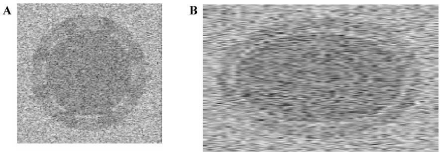
Orthogonal cross sections of the 3D synthetic dataset. 1A illustrates a "short-axis" slice through the data, 1B illustrates a cross section of the "long axis".

B. In vivo study

To test the efficacy of conservation of volume as a metric for accuracy of the segmentation algorithm in vivo, we studied three healthy, C57BL6 mice (Jackson Laboratories, Bar Harbor, ME). Each mouse was anesthetized using an isoflurane / atmospheric air mix and placed on a translation stage for precise image slice location. The mouse core temperature was monitored and maintained at 37.0±0.2°C using a heater built into the translation stage. Carefully maintaining the level of anesthesia and temperature ensures that the physiological condition of the mouse (i.e. principally heart rate) is maintained within a narrow range for the duration of the scanning. The study was performed in accordance with a protocol approved by the University of Virginia Animal Care and Use Committee. Each mouse was scanned using a high-frequency (30 MHz, 50% fractional BW) VisualSonics Vevo 770 scanner. The single-element, mechanically-swept transducer possessed 6.0 mm diameter and 12.7 mm focal depth. The transducer was used to acquire a high-resolution (50 µm axial, 100 µm lateral) short-axis B-mode image sequence at the base of the heart. Using the scanner's "ECG based Kilo-Hertz Visualization" (EKV) function, we acquired approximately 110 frames per heart cycle [24]. The mouse was translated in 1.0 mm increments and a new image sequence was acquired at each position, producing eight equally-spaced, parallel image sequences from base to apex of the left ventricle. Speckle-reducing anisotropic diffusion (SRAD) was applied to each image sequence offline in order to reduce speckle-induced errors in the segmentation algorithm [25]. SRAD uses the partial differential equation framework governing conventional anisotropic diffusion in conjunction with a specialized diffusion coefficient that promotes diffusion in homogenous regions and inhibits diffusion at edges, thereby preserving and enhancing edge regions in the image data. Corresponding frames were taken from each time step, assembled in a 3D matrix, and interpolated to form a full 3D data set.

C. Automatic segmentation

For both the synthetic data and in vivo studies, the epicardium was segmented using the same set of active surface parameters - specifically, 0.08, 0.2, 1.0, and 0.2 were used for the tension (α), rigidity (β), temporal step-size (τ), and GVF weighting parameter (μ), respectively. The epicardial surface is approximately a uniform curved surface, with relatively little signal dropout in the image data set; thus, the 3D GVF active surface converged accurately and quickly (within few iterations) given this "typical" set of surface parameters. Meanwhile, accurate segmentation of the endocardial border requires careful tuning of the active surface parameters because of signal dropout and complex geometry (i.e. the papillary muscles extend inwards as a pair of well defined bulges). Thus, we applied the principle of conservation of myocardial volume to adjust the parameters of the endocardial GVF active surface. An initial survey study was performed on representative simulated and in vivo data sets to determine the minimum and maximum possible values for each of the four parameters under consideration - the tension (α) and rigidity (β) of the active surface, the temporal step-size (τ), and the GVF field weighting parameter, μ. Beyond these limits, the active surface was found to either “collapse” (i.e. shrink until the surface disappeared entirely), “explode” (i.e. expand beyond all reasonable limits), or converge to a shape bearing no resemblance to the underlying source data. To investigate the behavior of the active surface over a the complete range of possible values for each parameter, the remaining three parameters were fixed at the midpoint of their respective ranges, and the parameter in question was adjusted, logarithmically, over ten values between that parameter's minimum and maximum.

For each set of active surface parameters in question, the two myocardial surfaces was segmented according to the temporally propagated GVFAS algorithm described in [26] (summarized in Fig. 2):

1. For the initial time step (representing end diastole), the user initializes the active contour model with a series of eight parallel circles, corresponding approximately with the shape and location of the epicardium in each of eight short-axis 2D cross sections of the data set between base and apex. During the in vivo study, these cross sections were the actual B-mode images obtained using the transducer.

2. Using this initial model, the GVFAS algorithm was iterated until convergence (i.e. approximately 20 iterations) to segment the epicardial surface at the first time step.

3. This surface was used to initialize the epicardial surface at the second time step. The GVFAS algorithm was iterated until convergence, producing a model of the epicardium at this time step. This model was used to initialize the third time step, and so on, until the epicardium had been segmented over the complete heart cycle.

4. The endocardial border was initialized at the first time point according to the process described in step 1.

5. Using this initial model, the GVFAS algorithm was iterated until convergence to segment the endocardial surface over at the first time step.

6. In some regions, the endocardial model expanded and incorrectly converged to the epicardial region of the image data set. The epicardial border (segmented in steps 2–3) was used to correct these errors in the endocardial model, "pushing" these local erroneous regions back towards the center of the model (the GVFAS algorithm was able to identify the epicardial border with greater accuracy than the endocardial border as the epicardial border region was less susceptible to signal drop-out and smoother in shape).

7. The corrected endocardial border was used to initialize the endocardial surface at the second time step. The GVFAS algorithm was iterated until convergence, producing a model of the endocardium at this time step. This model was corrected according the process described in step 6, used to initialize the third time step, and so on, until the endocardium had been segmented over the complete heart cycle.

Fig. 2.

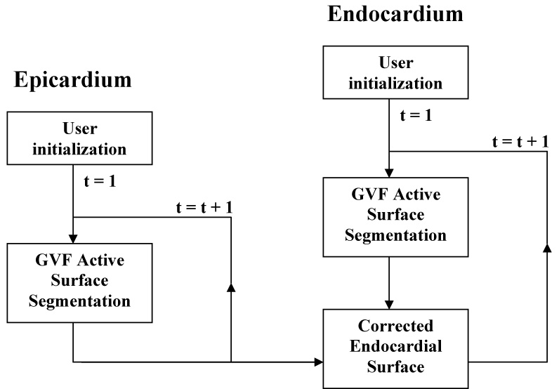
Schematic of the temporally propagated GVFAS algorithm.

The volumes contained within the epicardial and endocardial surfaces at each time point were computed. The difference between these volumes was multiplied by the myocardial density (1.05 g/mL [3]) to obtain the myocardial volume. Conservation of volume was evaluated by computing the ratio of the standard deviation of myocardial mass over the complete heart cycle to the mean myocardial mass. For the simulation data, the degree of conservation of volume was analyzed and the accuracy of the segmented model volume compared to the known true volume of the source data.

For the in vivo study, each 3D dataset was segmented manually by identifying the border of each endocardial and epicardial surface in a series of cross sections through the data. Two metrics were used to compare automatically segmented models to the manual segmentation of the left ventricle of each mouse. The Hausdorff distance [27] is the maximum distance between any point in each automatically segmented model to the closest respective point in the manually segmented model. The Hamming pseudo-distance [28] is the percentage of points on each automatically segmented model which are larger than D pixels (here, five) from the manually segmented model. For both metrics, lower values indicate greater similarity between a pair of models.

IV. Results

For the initial survey study, the tension of the active surface, α, was found to vary from approximately 0.01 to 0.10 for all synthetic and in vivo studies‥ Beyond these limits, the active surface would either collapse or explode. Thus, the logarithmic "midpoint" value used for α while adjusting the other parameters was 0.03. The rigidity of the active surface, β, was varied from 0.1 to 0.9. Beyond these limits, the active surface would either get become warped around image speckle or other noise sources (rather than conforming to image features) or collapse to a sphere. Therefore, the midpoint value for β was 0.30 when examining variations in other parameters . The temporal step-size parameter, τ, was varied from 0.001 to 10, beyond which the model would either deform so slowly that iterating the model until convergence became infeasible, or would deform too rapidly and overshoot edge regions in the gradient vector field. The midpoint value used for τ was 0.6. The weighting parameter of the gradient vector field, μ, varied from 0.03 to 1.4. Outside of these limits, the model would either converge to a shape bearing little resemblance to the source data or become warped around image speckle or other noise sources. The midpoint value used for μ was 0.2.

Each parameter was adjusted over the range of stable values while the other three parameters were fixed at their midpoint values. The time-propagated GVFAS algorithm was performed for each value of each parameter. The variation in volume (that is, the ratio of the standard deviation of volumes for the region between the endo- and epicardial surfaces over the complete cardiac cycle to the mean volume) for each parameter tested is presented in Fig. 3–Fig. 6 (note that a small value for volume variation corresponds with strong conservation of volume).

Fig. 3.

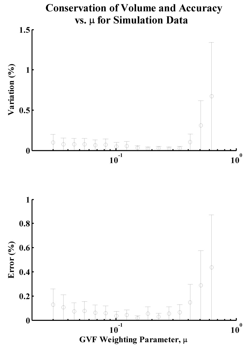
Variation in volume and error of mean volume over the range of investigated values for the GVF parameter, μ, for simulation data. Note that the plots have minima for approximately the same value of μ, indicating that strong conservation of volume corresponds with high accuracy of the model volume to the true volume of the synthetic data set.

Fig. 6.

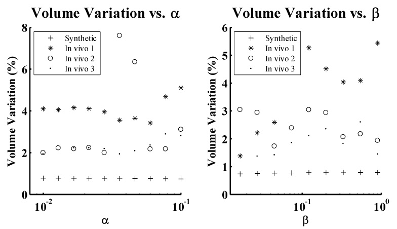
Variation in volume over the range of values investigated the active surface tension (α) and rigidity (β) parameters.

Both the variation and accuracy of the myocardial volume for each value of the parameter μ exhibited local minima for values of μ between 0.16 and 0.18 for synthetic data. In vivo, the variation in myocardial volume was minimal at approximately μ = 0.10 for the three data sets. Both Hamming and Hausdorff distances are smallest at or near this value of μ. A 2D, short-axis slice of one of the 3D in vivo data sets is presented in Fig. 7A for μ = 0.8 (a non-optimal value predicted by the metric), illustrating relatively poor accuracy of the endocardial model.

Fig. 7.

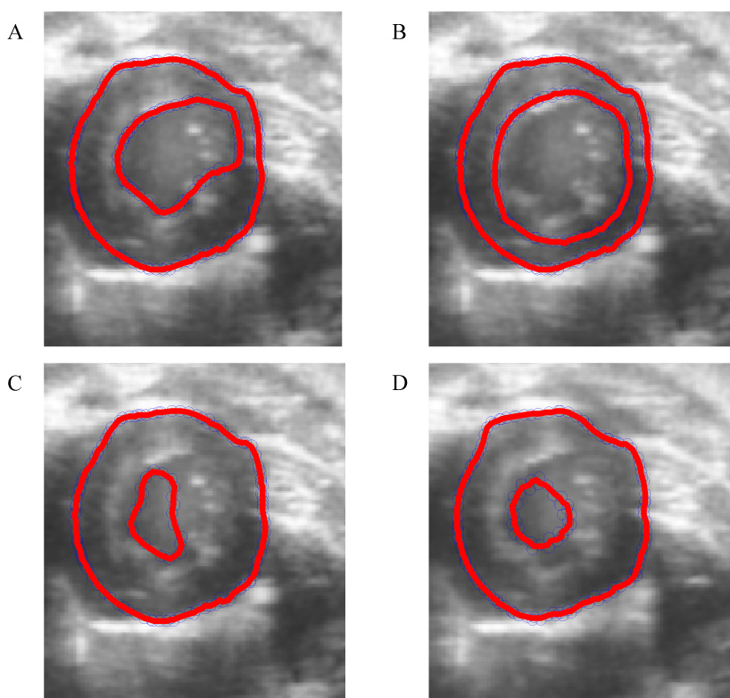
Midventricular slices through one of the three 3D in vivo image datasets, with superimposed 2D cross sections of the corresponding 3D active surfaces for both the epicardium and endocardium. Figs. 7A–D illustrate poorly-converged models corresponding with non-optimal values for each of the four parameters under consideration. 7A illustrates a an endocardial segmentation resulting from a non-optimal μ value of 0.80 - the right-hand side of the border becomes "stuck" in the myocardium. 7B illustrates segmentation resulting from a non-optimal τ value of 0.001, which yielded a contour which does not move quickly enough to track the contour from ED to ES. 7C illustrates the effect of extreme values of the α parameter (specifically, α = 0.1) - the high tension value pulls the contour away from the endocardial surface. 7D illustrates the effect of extreme values of the parameter β (specifically, β = 1.28) - at these values, the snake collapses as the tracking algorithm approaches end systole, eventually vanishing completely.

The active model converged quickly (i.e. within few iterations) to the synthetic target data for all investigated values of the temporal step size parameter τ, resulting in relatively constant volume variation over the range and rendering optimization of this parameter unnecessary for the data set. The active model surfaces exhibited local minima in variation in volume for the in vivo data set for values of τ between 0.06 and 0.17. Both Hamming and Hausdorff distances were minimal at these values of τ. A short-axis slice illustrating poor segmentation, corresponding with a value of τ = 0.001, is presented in Fig. 7B. 2D short axis slices illustrating surfaces generated by optimal values of μ = 0.10 and τ = 0.17 (and the "midpoint" values of α = 0.03 and β = 0.30) are presented in Figs. 8A–B at end diastole and end systole, respectively, illustrating an endocardial surface that accurately reflects the shape and features of the underlying B-mode image data. Full 3D active surface models generated by optimal parameters for in vivo and synthetic data are presented in Figs. 8C–D.

Fig. 8.

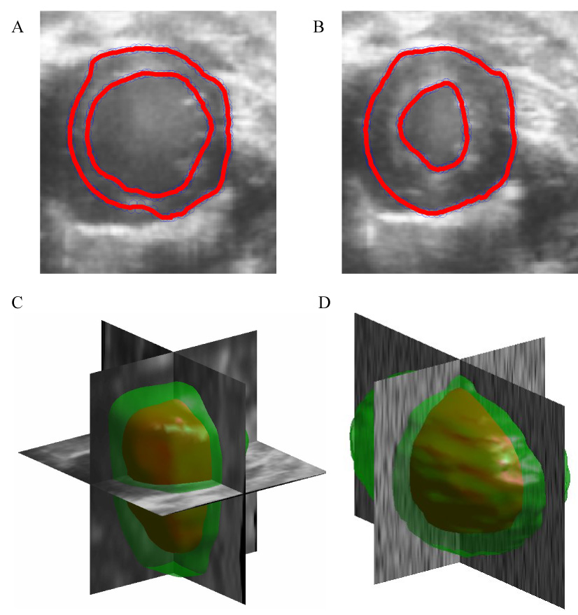
8A and 8B illustrate 2D short-axis slices of well-converged models at end diastole and end systole, respectively, resulting from a GVF weighting parameter μ of 0.10 and a temporal time step τ of 0.17. 8C and 8D illustrate full 3D reconstructions of the synthetic and in vivo data for optimal values of μ and midpoint (synthetic) and optimal (in vivo) values of τ, as predicted by the conservation of volume metric.

Volume variation remained relatively constant over all values investigated for the parameter α for both in vivo and synthetic data – although the exceptionally large values using in vivo data set 2 were the result of the endocardial active surface collapsing near end systole, as illustrated in Fig. 7C. Volume variation over the range of values investigated for the parameter β exhibited trends that, while not entirely random, did not correspond with accuracy of the GVFAS algorithm. For extremely large values of β, the active surface would collapse to a rigid, small sphere, as illustrated in Fig. 7D.

V. Discussion

It was found that conservation of volume was a useful predictor for the accurate selection of the GVF weighting parameter μ and the temporal step-size parameter τ. In the synthetic data study, models generated using the GVFAS algorithm exhibited the least variation in volume when μ was between 0.16 and 0.18, indicating that the algorithm was able to most effectively track the synthetic data for this range of values of μ. The models generated for these values of μ were also the most accurate, indicating that a GVFAS with a μ parameter which exhibits the least variation in volume (greatest conservation of volume) is the most accurate segmentation of the image data. This is confirmed when comparing automatically and manually segmented models for the in vivo data. The GVFAS generated by the value of μ which exhibited the greatest conservation of volume (μ = 0.10) accurately segmented the image data, closely mirroring automatically segmented models of the endocardial border and yielding small Hamming and Hausdorff distances. GVF active surfaces which exhibited poor conservation of volume were malformed in certain sections of the model and corresponded less accurately with the underlying image data, resulting in larger Hamming and Hausdorff distances.

The active surface model converged quickly (i.e. within few iterations) for the synthetic data sets for all investigated values of the temporal step-size parameter τ due to the relatively uniform, round shape of the synthetic target data. Thus, variation in volume remained consistently low over the entire range of values. Meanwhile, for the in vivo data sets, the active contour algorithm generated models which exhibited greatest conservation of volume for τ values of 0.06–0.17. These models represented accurate segmentation of the image data, yielding small Hamming and Hausdorff distances. Conversely, active surfaces which exhibited poor conservation of volume would either fail to converge to any shape at all or converge to an amorphous ellipsoid which did not resemble the image data, resulting in larger Hamming and Hausdorff distances.

In the evaluation of the two active surface parameters, tension (α) and rigidity (β), conservation of volume was found to be a poor predictor of accuracy of the GVFAS algorithm due to several complicating factors. Behavior of the algorithm over the range of values investigated for α approximated to "all or nothing". While the model would “collapse” or “explode” for extremely small or large values of α (and in unusual mid-range values for the second in vivo data set), performance of the algorithm remained consistently strong between these extremes, exhibiting only small, random changes.

For the rigidity parameter β, behavior of the algorithm exhibited trends in which strong conservation of volume did not necessarily correspond with accuracy of the model. The model exhibited strong conservation of volume at extremely low values of β due to superior ability to accurately segment the well-defined midventricular region of the 3D image data set. However, performance of the model was poor at the base and apex regions of the heart (where the underlying image data was more obscured by noise and signal drop-out), exhibiting random fluctuations and artifacts between time points in the cardiac cycle. Conservation of volume was again strong for higher values of β, which produced a model which was extremely smooth and nearly spherical. This model was also inaccurate, failing to correctly segment the complex geometry of the myocardium.

VI. Conclusion

We have demonstrated that conservation of volume is a useful metric for optimizing parameters when the GVFAS algorithm is applied to endocardial surface identification in 3D ultrasound image data. Specifically, the approach assists with appropriate selection of the GVF weighting parameter μ and the temporal step-size parameter τ. The metric was able to assess the efficacy of a wide range of potential values for these parameters and accurately identify the values which yielded the most accurate segmentation model in synthetic and in vivo data for μ and in vivo data for τ, indicating that metric should be effective across data sets acquired under diverse conditions. The algorithm is currently implemented in MATLAB to enable convenient “tuning” of the algorithm. However, it is currently a time-consuming process to test permutations of initialization parameters. The computation of a complete set of time-propagated GVFAS segmentations using a particular set of parameters takes one to two hours, limiting the quantity of synthetic and in vivo data sets which could be processed within a reasonable amount of time. Optimized implementation in C++ running on parallel processors could improve performance substantially, enabling efficient and more rigorous analysis over a greater quantity of data sets. With properly selected parameters, the GVFAS algorithm should provide an acceptable alternative to time-consuming manual segmentation, reducing the amount of time needed for data processing and reducing or eliminating user bias. While current work has focused on murine cardiac imaging, the algorithm and techniques described can be applied to human cardiac studies as well, where 3D echocardiography datasets have become available. Additionally, the a priori knowledge regarding conservation of myocardial volume through the cardiac cycle can also be applied to endocardial segmentation using other algorithms and imaging modalities.

Fig. 4.

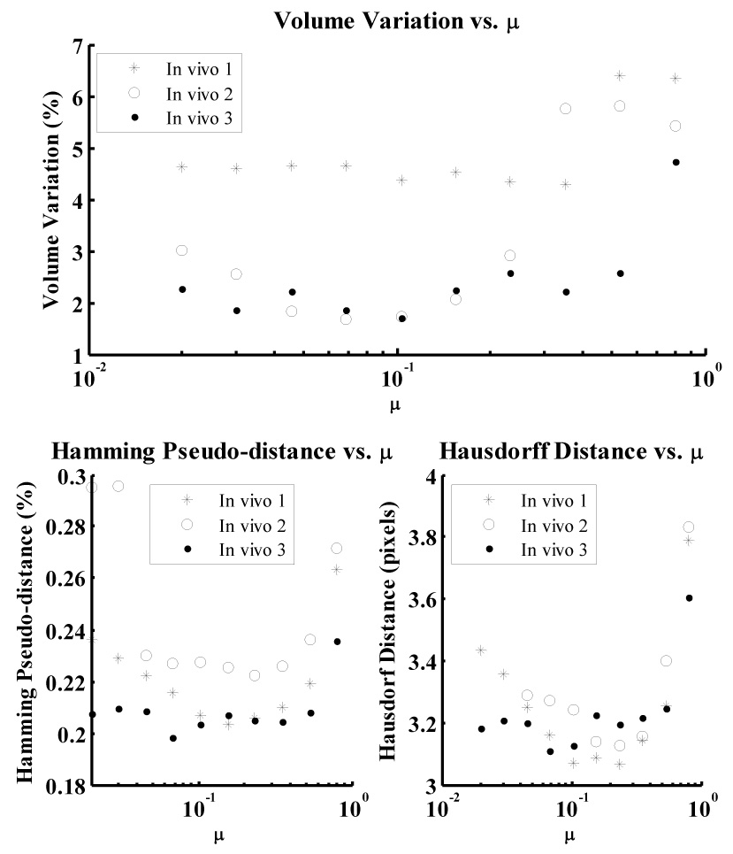
Variation in volume (i.e. the inverse of conservation of myocardial volume) over the range of values investigated for GVF weighting parameter μ for in vivo data. The Hamming pseudo-distance and Hausdorff distance, computed by comparing each model with manually segmented data, are also presented.

Fig. 5.

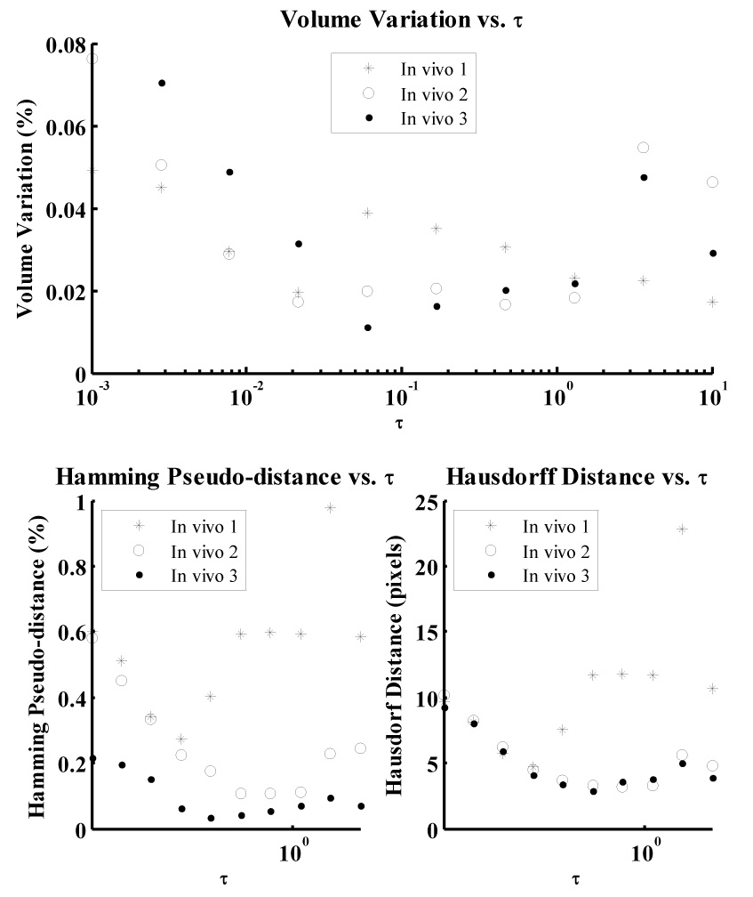
Variation in volume (i.e. the inverse of conservation of myocardial volume) over the range of values investigated for temporal step-size parameter τ for in vivo data. The Hamming pseudo-distance and Hausdorff distance, computed by comparing each model with manually segmented data, are also presented.

Biographies

Christopher D. Garson was born in Louisville, KY, in 1982. He earned his B.S. degree in biomedical engineering at Duke University, Durham, NC, in 2004. He is currently pursuing a Ph.D. degree in biomedical engineering at the University of Virginia, Charlottesville, VA. His doctoral research is focused on 3-D ultrasound and high-frequency murine cardiac imaging. His research interests include ultrasonic imaging, motion estimation, and image processing/segmentation.

Bing Li received the B.S. degree in Electrical and Computer Engineering from Peking (Beijing) University, Beijing, China in 2003. He received the M.S. and Ph.D. degrees in Electrical Engineering from the University of Virginia, Charlottesville, VA in 2005 and 2007, respectively. He is working in the RAPID division for KLA-Tencor Corporation. His research interests include medical image analysis, image segmentation, active models, and target tracking.

Scott T. Acton graduated from Oakton High School, Vienna, Virginia, in 1984. He received the B.S. degree in Electrical Engineering from Virginia Tech, Blacksburg in 1988 as a Virginia Scholar. Dr. Acton received the M.S. degree in Electrical and Computer Engineering and the Ph.D. degree in Electrical and Computer Engineering from the University of Texas at Austin in 1990 and 1993, respectively, where he was a student of the great Al Bovik.

Dr. Acton has worked in industry for AT&T, Oakton, Va., the MITRE Corporation, McLean, Va. and Motorola, Inc., Phoenix, Az. and in academia for Oklahoma State University, Stillwater. Currently, he is Professor of Electrical and Computer Engineering and Biomedical Engineering at the University of Virginia (U.Va.). At U.Va., he was named the Outstanding New Teacher in 2002, Faculty Fellow in 2003, and Walter N. Munster Chair for Intelligence Enhancement in 2003.

Dr. Acton is an active participant in the IEEE, currently serving as Associate Editor for the IEEE Transactions on Image Processing and, formerly, as Associate Editor the IEEE Signal Processing Letters. He was the 2004 Technical Program Chair and the 2006 General Chair for the Asilomar Conference on Signals, Systems and Computers. His research interests include anisotropic diffusion, basketball, active contours, biomedical segmentation problems and biomedical tracking problems. He lives in beautiful Charlottesville, Virginia, with his wife and two boys.

John A. Hossack was born in Glasgow, Scotland, in 1964. He earned his B.Eng. Hons(I) degree in electrical electronic engineering from Strathclyde University, Glasgow, in 1986 and his Ph.D. degree in the same department in 1990. From 1990 to 1992, Dr. Hossack was a post doctoral researcher in the E. L. Ginzton Laboratory of Stanford University working under B. A. Auld’s guidance. His research was on modeling of 0:3 and 1:3 piezoelectric composite transducers. In 1992, he joined Acuson, Mountain View, CA, initially working on transducer design. During his time at Acuson his interests diversified into beamforming and 3-D imaging. Dr. Hossack was made a Fellow of Acuson for ‘excellence in technical contribution’ in 1999. In 2000 he joined the Biomedical Engineering Department at the University of Virginia, Charlottesville, VA. His current interests are in improved 3-D ultrasound imaging and high bandwidth transducers/signal processing.