Reconstruction of central cortical surface from brain MRI images: Method and application

Abstract

Reconstruction of the central surface representation of the cerebral cortex is an important means to study the structure and function of the human brain. In this paper, we propose a novel method based on an elastic transform vector field to drive a deformable model for the reconstruction of the central cortical surface. Both simulated brain cortexes and real brain images are used to evaluate this approach. We applied the surface reconstruction method and a hybrid volumetric and surface registration algorithm to detect simulated brain atrophy. Experimental results show that the central cortical surface representation has better performance in detecting simulated atrophy than the traditionally used inner or outer cortical surface representations.

Introduction

The human cerebral cortex can be described as a thinly folded two-dimensional sheet with a highly folded and curved geometry (Van Essen and Maunsell, 1980; Xu, 1999; Xu et al., 1999; Fischl et al., 1999). Reconstruction and representation of the cerebral cortex from MR images play an important role in the study of structure and function of the brain (Van Essen et al., 2001; Fischl et al., 2002; Thompson et al., 2003; Miller 2004; Chung et al., 2005; Thompson et al., 2005). In recent years, there has been significant effort towards the development of methods for reconstruction of the cortical surface. Most of these methods are either voxel-based or deformation-based (Mangin et al., 1995; Davatzikos and Bryan, 1996; Zeng et al., 1998; Xu et al., 1999; Fischl et al., 1999; Dale et al., 1999; Miller et al., 2000; Shattuck and Leahy, 2001; Shattuck and Leahy, 2002; Han et al., 2003; Thompson et al., 2005; Kim et al., 2005; Xu et al., 2006). The homotopically deformable model developed in Mangin et al., 1995 is one of the earliest examples of voxel-based methods. This method starts with an initial region with the required topology and then grows the region by adding simple points (Kong and Rosenfeld, 1989), whose addition or removal will not change the topology. The algorithm proposed by Shattuck and Leahy 2001 is another example of the voxel-based method, in which the voxel connections can be corrected locally to obtain a topologically spherical surface by using the Marching Cubes technique introduced in (Lorensen and Cline, 1987; Montani et al., 1994). Instead of reconstructing the surface from boundary voxels directly, deformation-based methods deform an initial surface continually to the true surface (Davatzikos and Bryan, 1996; Sandor and Leahy, 1997; Xu et al., 1999; MacDonald et al., 2000; Thompson, 2005; Kim et al., 2005; Xu et al., 2006). More specifically, deformable surfaces could be categorized into parametric models and geometric models. An advantage of the parametric surface model is that the topology of the final surface is identical to that of the initial one, provided that the deformation is topology-preserving (Davatzikos and Bryan, 1996; MacDonald et al., 2000). Alternatively, geometric deformable models could be used to generate topologically correct cortical surfaces (Zeng et al., 1998; Han et al., 2003). In particular, a topology-preserving geometric model was introduced to reconstruct the inner, outer, or central cortical surfaces in Han et al., 2003.

The central cortical layer is defined as the layer lying in the geometric center of the cortex, which is approximately the cytoarchitechtonic layer four (Xu et al., 1999). Comparing to the inner cortical (WM/GM interface) and outer cortical (GM/CSF interface) surfaces, the surface defined on the central layer could provide considerably better geometric information of the cortex (Van Essen and Maunsell, 1980; Drury et al., 1996; Xu et al., 1999). Although a variety of methods have been suggested to effectively deal with the reconstruction of the inner and outer cortical surfaces, only a few works have been done to generate the central cortical surface, e.g., Xu et al., 1999 proposed a deformable surface model by using the gradient vector flow to obtain the central cortical surface, and Fischl et al. 2000 defines the central surface as the interim surface that resides on the half way when deforming from the inner surface to the outer surface. In this work, we employed an elastic deformable transform (EDT) model, which is adopted from continuum mechanics as in Kass et al. (1987), to drive a deformable model for the reconstruction of central cortical surface. To evaluate the accuracy of our central cortical surface reconstruction algorithm and compare it with the existing methods, we propose an approach that generates a simulated brain cortex, in which the ground truth of the central cortical layer is already known. The evaluation results demonstrate reasonably good performance of the proposed reconstruction method. Finally, the central surface reconstruction and representation method is applied to detect simulated brain atrophy. Our preliminary results show that the central cortical surface provides better performance in detecting differences in normal brains and atrophied ones than traditionally used inner or outer cortical surfaces.

Methods

Overview

The computational framework of the central cortical surface reconstruction is composed of five steps, as summarized in Fig. 1. The first step automatically performs skull-striping and segments the Spoiled Gradient Echo (SPGR) brain image into distinct compartments of CSF, GM, and WM. The second step performs topology correction to the WM and GM images in order to obtain zero genus volumes. Afterwards, the inner cortical surface is reconstructed using the marching cubes algorithm in the third step. The fourth step performs an elastic transformation on the topologically corrected GM/WM volume images to generate a smooth deformation field. Finally, we apply the deformation field on the inner surface to deform it towards the central layer of the cortex, represented by Step 5 in Fig. 1.

Fig. 1.

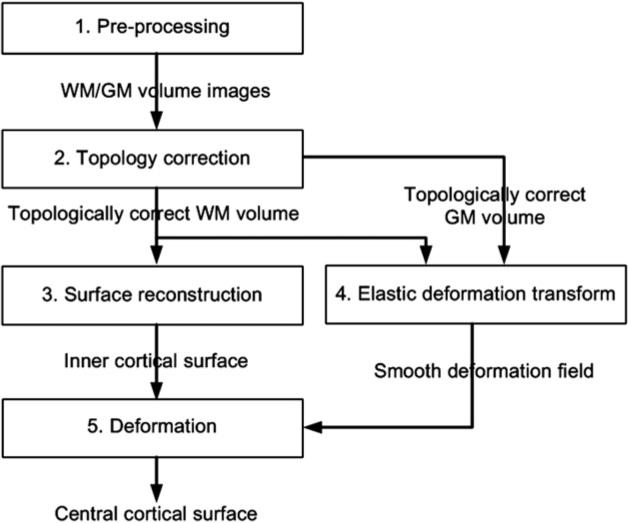
An overview of the central cortical surface reconstruction procedure.

Pre-processing

We utilize the Oxford FSL tools (http://www.fmrib.ox.ac.uk/fsl/) for preprocessing and brain segmentation of the volumetric MR images. First, we use the Brain Extraction Tool (BET) to remove the non-cerebral tissues including bone, skin, fat, etc. Since our surface reconstruction algorithm only tests the cerebral cortex, the cerebellum and brain stem are also removed using in-house developed tools. We then use the automated segmentation tool, FAST, to segment the brain into GM, WM, and CSF compartments, where the spatial bias is corrected simultaneously.

Generation of inner cortical surface with correct topology

As illustrated in Fig. 2c, due to the partial volume effect and the narrow sulci, part of the deep buried sulci might become connected (Mangin et al., 1995). When initialized from the outside of the cortical surface, the deformable surfaces have difficulty in progressing into the sulci (Xu et al., 1999; Davatzikos and Byran, 1996). As suggested in Xu et al. (1999), the inner cortical surface is generated as the initial surface, because of its closeness to the cortex.

Fig. 2.

Generation of the inner cortical surface. (a) A slice of MRI image after removal of non-cerebral tissues. (b) Segmented result of (a). (c) The zoomed-in version of the marked region in (a) and (b). (d) The inner cortical surface.

Reconstructing a topologically correct and geometrically accurate inner surface is an important issue. Shattuck and Leahy (2001) presented an automated graph-based algorithm for topology correction in a binary volume image. The graphs are constructed to represent the connectivity of both foreground and background voxels respectively. If the expected surface is homeomorphic to a sphere, assuming that no cycle exists in the connectivity graphs, the handle-removing problem can be considered as removing the cycles in the connectivity graphs. This assumption was later proved to be correct by Abrams et al. (2002). The graph-based method operates on the voxel membership set of the volume and makes minimal changes to force it to have the topology of a sphere (Shattuck and Leahy, 2001). After the topology correction step is completed, a voxel-based method, such as the Marching Cubes algorithm (Lorensen and Cline, 1987), can be used to reconstruct an isosurface of the corrected volume. In our experiments, the BrainSuite (Shattuck and Leahy, 2002) tools that implemented the algorithm in Shattuck and Leahy (2001) are used to remove the topology errors and to generate the inner cortical surface.

Reconstruction of central cortical surface

Deformable model

The deformable model introduced in (Kass et al., 1987; McInerney and Terzopoulos, 1996) is adopted in this paper. It deforms a parameterized surface x(u) = [x(u), y(u), z(u)]^T, u= (u₁, u₂) ∈[0, 1] × [0, 1] in the spatial domain to minimize the energy function:

$$E=\int \frac{1}{2}\left(\alpha \sum _{i=1}^2{\mid {\mathbf{x}}_i\mid }^2+\beta \sum _{i,j=1}^2{\mid {\mathbf{x}}_{ij}\mid }^2\right)+E_{ext}\left(\mathbf{x}\right)d\mathbf{u}$$ (1)

where parameters α and β control the tension and rigidity of the surface, respectively. Symbols x_i and x_ij denote the first and second derivatives of x to u_i, and E_ext(x) is the external energy derived from the image. The solution to the minimization problem should satisfy the Euler equation:

$$F_{\mathrm{int}}+F_{\mathrm{ext}}=0$$ (2)

where F_int = αΔ_ux − βΔ_u(Δ_ux) and F_ext = −∇E_ext(x) are defined as the internal and external forces respectively, Δ_u = ∂²/(∂u₁)² + ∂²/ (∂u₁)² is the Laplacian operator, and ∇ is the gradient operator. The steady-state solution of the dynamic equation yields:

$${\mathbf{x}}_t=F_{\mathrm{int}}+F_{\mathrm{ext}}$$ (3)

where the surface x is treated as a function of time t.

The deformable model encounters difficulties in progressing into boundary concavities when reconstructing the central surface (Davatzikos and Bryan, 1996). In order to deal with this problem, an external force field v, called gradient vector flow (GVF), is proposed in (Xu and Prince, 1998). In this method, the external force is not constrained to be a gradient vector of the scalar field E_ext(x) and could be defined by various vector fields if necessary. Here, we first briefly discuss the GVF method proposed in (Xu et al., 1999; Xu and Prince, 1998). Subsequently, we introduce our external force used for the deformable surface model.

Gradient vector flow and generalized gradient vector flow

The Gradient Vector Flow (GVF) field is defined as the solution of the following Euler equation:

$$\mu \Delta v-{\mid \nabla f\mid }^2(\mathbf{v}-\nabla f)=0$$ (4)

where μ is the regularization parameter, Δ is the Laplacian operator, and f is defined as the segmented GM image, where voxels are set either to zero or one. Applying Eq. (2), the solution can be shown to satisfy the following dynamic equation:

$$\{\begin{array}{c}{\mathbf{v}}_t=\mu \Delta v-{\mid \nabla f\mid }^2(\mathbf{v}-\nabla f)\hfill \\ \mathbf{v}(\mathbf{x};0)=\nabla f\hfill \end{array}\phantom{\}}$$ (5)

where v_t denotes the partial derivative of v(x;t) with respect to time t. More details about the GVF method can be found in Xu and Prince (1998). After the introduction of GVF, the generalized gradient vector flow (GGVF) was proposed in Xu et al., 1999. GGVF is defined as the solution of the following Euler equation:

$$\{\begin{array}{c}{\mathbf{v}}_t=g(\nabla f)\Delta \mathbf{v}-h(\nabla f)(\mathbf{v}-\nabla f)\hfill \\ \mathbf{v}(\mathbf{x};0)=\nabla f\hfill \end{array}\phantom{\}}$$ (6)

where g(x) = exp( −(x/k)²) and h(x) = 1 − g(x), k is a scalar. Compared to GVF, this method improves the convergence properties the narrow concavities.

Elastic deformation transform

Under the elastic deformation transform (EDT), images are modeled as elastic objects warped by an external force field. This method was introduced in Davatzikos et al. (1996) as a registration model, where the deformation of the boundary voxels is pre-fixed. The EDT model is defined as:

$${\mu }_{\mathrm{e}}\Delta \mathbf{v}+({\lambda }_{\mathrm{e}}+{\mu }_{\mathrm{e}})\nabla \mathrm{div}\mathbf{v}+q(x,y,z)(\nabla f-\mathbf{v})=0$$ (7)

where div is the divergence operator, μ_e and λ_e are the elasticity parameters (known as the Lame moduli (Gurtin, 1981)), and q(x,y,z) is an indicator function, which specifies whether the displacement is pre-fixed at the position. In our work, the indicator function is set as

$$q(x,y,z)=\{\begin{array}{cc}1\hfill & \mid \nabla f(x,y,z)\mid >0\hfill \\ 0\hfill & \text{otherwise}\hfill \end{array}\phantom{\}}$$ (8)

This model can be solved to obtain the following dynamics:

$$\{\begin{array}{c}{\mathbf{v}}_t={\mu }_{\mathrm{e}}\Delta \mathbf{v}+({\lambda }_{\mathrm{e}}-{\mu }_{\mathrm{e}})\nabla \mathrm{div}\mathbf{v}+q(x,y,z)(\nabla f-\mathbf{v})\hfill \\ \mathbf{v}(\mathbf{x};0)=\nabla f\hfill \end{array}\phantom{\}}$$ (9)

where v_t denotes the partial derivative of v(x;t) with respect to time t.

The solution of Eq. (7) defines the displacement of each position in an elastic object, when the boundary displacement is prefixed. Let us consider v in Eq. (7) as a velocity field instead of a displacement field. Then, when compared with Eq. (4), only the second term is added to the EDT model in Eq. (7). According to hydromechanics, the second term in Eq. (7) denotes the compression of a compressible fluid, and div v = 0 means the uncompressible fluid. The second term of Eq. (7) is responsible for making v smoother in space. As shown in Xu et al., 1999, the gradients at the each side of the thick boundary are converged to the center layer by the GGVF method. Since the EDT method has similar gradient diffusion capability as the GGVF method but in a smoother way, the EDT method will presumably converge the gradient to the central layer, which will be demonstrated in Results.

Numerical implementation

The explicit finite difference scheme can be implemented for the 3 types of field above, as described in Xu and Prince (1998). The implementation is stable when the Courant–Friedrichs–Lewy (CFL) step-size restriction should be maintained:

$$\frac{g\Delta t}{\Delta x\Delta y\Delta z}\le C$$ (10)

where C is the CFL step-size restriction, Δt is the time step for each iteration, Δx, Δy and Δz are the spaces between voxels, and g is the maximum multiplying factor of Δv. In GGVF, the g value is almost set to 1 in smooth region, so compared to GVF and EDT, much smaller Δt should be set in GGVF to maintain CFL step-size restriction. Thus much more iterations are needed in GGVF.

Deformation using pressure force

In this work, we employ the balloon model in Cohen (1991). The balloon model uses pressure forces to deform a surface in order to increase its speed of convergence. This is done in cases where the deformable surface is far from the GM (Xu et al., 1999). Since the surface vertices move along with the normal direction in the balloon model, the shape of the initial surface is maintained.

In order to capture the GM, the surface is inflated inside the WM and deflated otherwise. Therefore, the pressure force can be defined as:

$$F_{\text{pressure}}={\omega }_3(2W\left(\mathbf{x}\right)-1)\cdot \mathbf{n}\left(\mathbf{x}\right)$$ (11)

where ω₃ is the force strength weight, W(x) is the WM indicator function, and n(x) is the outward unit normal vector of the surface at vertex x. To accurately trace the central layer in the GM, the pressure force is only adopted outside of the GM. The final force with pressure force is then given as:

$$F_{\mathrm{ext}}=G\left(\mathbf{x}\right)\cdot \mathbf{v}\left(\mathbf{x}\right)+(1-G\left(\mathbf{x}\right))\cdot F_{\text{pressure}}$$ (12)

where G(x) is the GM indicator function, and v(x) is the field defined in subsection 2.4.3.

Results

The central surface reconstruction method described in Subsection 2.4 is applied to the MRI brain images of ten subjects. The simulated GM volume image in each case was reconstructed using the method described in the following subsection 3.1.1. The parameters used in our experiments for the deformable model are: α=0.25 and β=0, for pressure force, ω₃=1.0 for GVF, μ=0.2, for GGVF k=0.2 and for EDT, μ_e = 0.2 and λ_e = 0.2.

Evaluation using the simulated cortex

Generation of the simulated brain cortex

Despite the existence of simulated brain datasets such as the BrainWeb (McConnell Brain Imaging Centre at McGill University) that can provide a true GM segmentation (Kwan et al., 1999), these datasets contain no true central surface. Xu and Prince (1998) proposed a landmark method for dealing with this problem, however, their technique involves marking the position of the entire central layer, which is time-consuming. In this work, we generate a simulated brain cortex where the central cortical layer is known.

The entire procedure is illustrated in Fig. 3. First, by using the methods in Subsections 2.4, we generate a central cortical surface that is close to the true central surface (Fig. 3a). Next, this triangulation surface is interpolated to a volume image (Fig. 3b). Given this, the central voxel set is defined as:

$$V_c=\{\mathbf{x}\mid \mathbf{x}\text{is a central voxel}\}$$ (13)

Fig. 3.

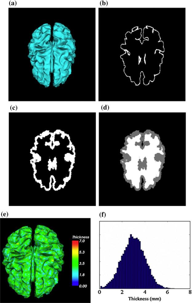
The simulated brain. (a) Central surface. (b) Interpolated to volume image. (c) The simulated GM. (d) The simulated brain. (e) Thickness over the central layer. (f ) Histogram of the thickness.

We defined a value for the thickness of the cortex on each voxel x_i in V_c. Since the thickness of the cortex varies over the brain, we used a Gaussian distribution to generate the thickness defined in our simulation. Following this assumption, the distribution is described as:

$$\text{Thick}\left({\mathbf{x}}_i\right)\sim N\left({\mu }_{\text{thick}},{\sigma }^2\right)$$ (14)

where μ_thick is the mean thickness of the cortex, and σ² is the variance of the thickness. In our experiments, μ_thick and σ² are set to be 3.0 mm and 1.0 mm² respectively. All thickness values, generated by Eq. (12), that are less than zero are clearly meaningless, and are consequently set to 0.1 mm. Fig. 3e and f illustrates the distribution of the thickness over the central surface. We then define the GM region near each central voxel x_i as follows:

$$\mathrm{GM}\left({\mathbf{x}}_i\right)=\left\{\mathbf{x}\mid \mid \mathbf{x}-{\mathbf{x}}_i\mid \le \frac{\text{Thick}\left({\mathbf{x}}_i\right)}{2}\right\}$$ (15)

Grouping all GM regions near each of the central voxels, we arrive at the simulated GM:

$$\mathrm{GM}=\underset{i=1}{\overset{N}{\cup }}\mathrm{GM}\left({\mathbf{x}}_i\right){\mathbf{x}}_i\in V_c$$ (16)

where N is the total number of central voxels. The simulated GM, as illustrated in Fig. 3c, is obtained after sampling the GM over the continuous region defined in Eq. (16). Although the simulated GM is quite different from the original brain, we believe that due to its very convoluted cortical surface, it is sufficient for the validation of our algorithm. Using the method introduced in Reconstruction of central cortical surface, we can obtain the central surface of the simulated GM.

Visual evaluation

In this section, we present the results obtained using the simulated brain cortex with and without pressure force as described in Reconstruction of central cortical surface. To evaluate the fidelity of the reconstructed surface, we compare the distance of the reconstructed central surface to the ground-truth central surface. We first define the distance from each vertex on the reconstructed surface Ω to the ground-true central surface Ω_t via:

$$d\left(\mathbf{x}\right)=\underset{{\mathbf{x}}_t\in {\Omega }_t}{\min }\mid \mathbf{x}-{\mathbf{x}}_t\mid$$ (17)

To facilitate our comparison of different results, the value of d(x) is truncated to 4.0 if it exceeds 4.0.

Fig. 4 shows the results obtained for both methods without pressure forces using GVF and EDT. The color-coded distance of the reconstructed central surface to the ground truth of the central layer using the GVF and the EDT methods are shown in Fig. 4a and b. It is obvious that employing the EDT method generates a central surface that is closer to the ground truth of the central layer. This can also be further confirmed by the histogram of distances in Fig. 4c and d. The average distance for the GVF method is 1.38 mm while the average distance for EDT is 0.84 mm.

Fig. 4.

Reconstruction of central surfaces from simulated brain cortex without pressure force. (a, b) Color-coded distance of reconstructed surfaces to the ground truth of the central layer using GVF and EDT. (c, d) Histograms of the distance to the central layer using GVF and EDT.

The results of the methods using the GVF and the EDT along with pressure forces in the deformable model are shown in Fig. 5. Comparing to the results obtained without employing pressure force (shown in Fig. 4), the method that employs pressure force results in a higher level of accuracy. The less concentrated red areas in Fig. 5 verify this claim. The average distance for GVF method is 0.93 mm while the average distance for EDT is 0.84 mm. This result shows that the EDT method performs better than the GVF method.

Fig. 5.

Reconstruction of the central surfaces of the simulated brain cortex with pressure force. (a, b) Color-coded distance of the reconstructed central surfaces to the ground-truth of central layer using GVF and EDT. (c, d) Histogram of the distance to the central layer using GVF and EDT.

Quantitative evaluation for ten subjects

Since the reconstructed central surface cannot completely converge into the GM, the percentage of the reconstructed surface vertices that fall outside the GM can serve as a good indicator for the evaluation of different reconstruction algorithms. The non-GM percentage η is defined as:

$$\eta =\frac{{\int }_{\Omega }(1-G\left(\mathbf{x}\right))dA}{{\int }_{\Omega }dA}\times 100\%$$ (18)

where Ω is the reconstructed central surface and G(x) is the GM indicator function.

The non-GM percentage values for the two methods using GVF and EDT are listed in Tables 1, 2, 3, 4. In the absence of pressure force, the EDT result is about 16% better than the GVF result (shown in Table 1). Although the pressure force improves the non-GM percentage results for the GVF method significantly, as shown in Table 2, the EDT method still performs better than the GVF method. These conclusions are also true for the results obtained using the simulated brain cortex, as shown in the second and third columns of Tables 3 and 4.

Table 1.

Non-GM percentages on original segmented cortex images without pressure force (%)

	1	2	3	4	5	6	7	8	9	10	Mean
GVF	26.0	29.6	31.0	29.0	26.2	34.7	25.8	26.6	26.0	27.5	28.2
EDT	11.1	12.1	15.2	12.4	12.1	16.9	9.9	10.7	10.5	10.4	12.1

Table 2.

Non-GM percentages on original segmented cortex images with pressure force (%)

	1	2	3	4	5	6	7	8	9	10	Mean
GVF	7.09	6.58	6.10	4.90	12.6	6.92	7.09	9.43	7.44	6.61	7.48
EDT	6.07	5.59	4.92	4.25	11.4	5.54	6.28	8.87	5.88	5.30	6.41

Table 3.

Measurements of the central surface on the simulated brain without pressure force

	η (%)		Aver (mm)		Max (mm)		Std (mm)
	GVF	EDT	GVF	EDT	GVF	EDT	GVF	EDT
1	19.53	0.91	1.49	0.85	7.30	4.20	1.25	0.49
2	17.39	0.41	1.39	0.81	8.33	4.09	1.29	0.44
3	15.70	0.59	1.35	0.83	7.48	3.36	1.23	0.46
4	15.36	0.34	1.32	0.83	8.20	3.48	1.23	0.44
5	15.19	0.42	1.32	0.82	8.64	3.43	1.30	0.44
6	16.42	0.99	1.41	0.88	8.36	4.03	1.21	0.50
7	18.83	0.50	1.43	0.83	8.82	4.23	1.21	0.45
8	15.49	0.45	1.34	0.83	9.12	3.12	1.21	0.44
9	17.00	0.58	1.38	0.86	8.30	3.83	1.24	0.46
10	17.59	0.54	1.41	0.82	8.53	3.56	1.27	0.44
Mean	16.85	0.57	1.38	0.84	8.31	3.73	1.24	0.46

Table 4.

Measurements of the central surface on the simulated brain with pressure force

	η (%)			Aver (mm)			Max (mm)			Std (mm)
	GVF	EDT	GGVF	GVF	EDT	GGVF	GVF	EDT	GGVF	GVF	EDT	GGVF
1	0.18	0.06	1.08	0.91	0.82	0.83	3.91	3.24	5.38	0.50	0.42	0.50
2	0.22	0.07	1.27	0.91	0.83	0.82	3.51	3.33	10.2	0.49	0.43	0.55
3	0.22	0.03	1.72	0.90	0.83	0.86	3.35	2.78	9.81	0.49	0.42	0.59
4	0.35	0.11	1.20	0.93	0.84	0.82	3.31	3.17	6.66	0.50	0.43	0.53
5	0.67	0.27	1.73	1.01	0.89	0.87	4.31	4.60	7.83	0.56	0.49	0.58
6	0.21	0.08	2.30	0.92	0.83	0.87	3.60	2.97	11	0.49	0.43	0.75
7	0.26	0.03	1.88	0.91	0.84	0.86	3.18	2.97	9.14	0.48	0.42	0.59
8	0.25	0.05	1.63	0.95	0.86	0.85	3.08	2.81	9.24	0.52	0.45	0.56
9	0.27	0.06	1.34	0.91	0.82	0.83	3.48	2.95	6.44	0.49	0.42	0.54
10	0.50	0.31	1.65	0.99	0.89	0.86	3.73	3.63	7.39	0.56	0.49	0.55
Mean	0.31	0.11	1.58	0.93	0.84	0.85	3.54	3.24	8.31	0.51	0.44	0.57
t-test	EDT<GVF		P=0.0012	EDT<GGVF		P=0.43	EDT<GVF		P=0.09	EDT<GVF		P=2e-5
	GVF<GGVF		P=4e-9	EDT<GVF		P=4e-6	GVF<GGVF		P=1e-7	GVF<GGVF		P=0.056

t-tests are performed to compare the different methods, and the P-values are presented.

Based on the minimal surface distance definition given in Eq. (15), we define the following global distance measurements: (a) Average distance (Aver)

$$\text{Aver}=\frac{{\int }_{\Omega }d\left(\mathbf{x}\right)dA}{{\int }_{\Omega }dA}$$ (19)

(b) Standard variance of distance (Std)

$$\mathrm{Std}=\sqrt{\frac{{\int }_{\Omega }{(d\left(\mathbf{x}\right)-\text{Aver})}^{2}dA}{{\int }_{\Omega }dA}}$$ (20)

(c) Maximal distance (Max)

$$\mathrm{Max}=\underset{x\in \Omega }{\max }d\left(\mathbf{x}\right)$$ (21)

The results of these three measurements are listed in Tables 3 and 4. The t-test is also applied to these measurements for group comparison. The results are provided in Table 4. The proposed EDT method, no matter whether with or without pressure force, produces a considerable good average distance to the central layer, which is about 0.84 mm. The pressure force deforms the surface more into the GM and improves these three measurements, especially for the GVF method. Notably, the reconstructed central surfaces have a systematic deviation towards the inside of the ground-truth central surface.

Evaluation using real brain MRI data

Visual evaluation

To visually evaluate the cortical surface reconstruction result, Fig. 6 provides an example of the outer, inner, and central cortical surfaces reconstructed from a high resolution brain MRI image (0.5 mm, isotropic). As clearly indicated in Fig. 6d where all of the three surfaces are embedded in the same volumetric slice, the central cortical surface resides in between the inner and outer surfaces. Since it is challenging to visually evaluate whether or not the reconstructed central cortical surface is really located in the central layer of cortex in 2D slice (Jones et al., 2000), only a few areas where the central surface looks to be centrally located are highlighted by red arrows in Fig. 6d. Notably, the central cortical surface (Fig. 6c) looks less convoluted than the inner cortical surface (Fig. 6b), but more convoluted than the outer surface (Fig. 6a). This partly indicates that the reconstructed central surface is located in between the inner and outer surfaces.

Fig. 6.

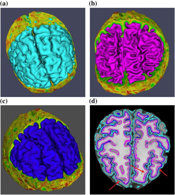
Cortical surfaces of the same subject. (a) Outer cortical surface. (b) Inner cortical surface. (c) Central cortical surface. (d) All of the three surfaces embedded into the volume slice.

Quantitative evaluation and comparison

In order to provide a quantitative evaluation of our techniques, we illustrate experimental results for two of the 10 subjects. The central surfaces deformed by GVF and EDT fields without pressure force (as described in Subsection 2.4) are shown in Fig. 7. The 3D views of the central surfaces are rendered in Fig. 7a and b. Compared with GVF, the central surface reconstructed using the EDT field provides better reconstruction of the central layer with significantly fewer voxels outside the GM. This is indicated by the less densely red-colored areas of Fig. 7b, comparing to that of Fig. 7a. Similar results are obtained for the second subject on the right column.

Fig. 7.

Results for two subjects of reconstructed central surface without pressure force. (a) Central surfaces by GVF. (b) Central surfaces by EDT.

The results of using the pressure force (as described in Subsection 2.4) combined with the deformable model are shown in Fig. 8. As is clear from Fig. 8, both GVF and EDT results are improved, comparing to the results presented in Fig. 7. The EDT method still performs better than the GVF method, as indicated by the quantitative results for nine cases in the first and second rows of Table 5. Compared to the results presented in Fig. 7, the improvement in the performance achieved in the central surfaces using GVF by applying pressure forces is higher than that achieved by using EDT. For example, the red areas in Fig. 8a are much less dense than those in Fig. 7a. Similar conclusions can be drawn for the second case shown in the right column of Fig. 8. It is evident that the central surface reconstruction method in Xu et al., 1999 using GVF relies much more on the pressure force to obtain a reasonably good result. The results in Figs. 7 and 8 suggest that the deformation force of the EDT has better performance in driving the deformable surface to the central layer of the GM.

Fig. 8.

Results for two subjects of reconstructed central surfaces with pressure force. (a) Central surfaces by GVF. (b) Central surfaces by EDT.

Table 5.

Non-GM percentage on original segmented cortex image with pressure force (%)

	1	2	3	4	5	6	7	8	9	Mean
EDT	6.07	5.59	4.92	4.25	11.4	5.54	6.28	8.87	5.88	6.41
GVF	7.09	6.58	6.10	4.90	12.6	6.92	7.09	9.43	7.44	7.48
FreeSurfer	8.33	7.68	5.33	6.41	10.6	7.2	23.2	7.83	5.64	9.14

The EDT and GVF methods are also compared with the central cortical surface reconstruction method used in the MGH FreeSurfer (Fischl et al., 1999; Dale et al., 1999). The procedure of the central cortical surface reconstruction using the FreeSurfer is briefly described as follows. First, the brain MR image is aligned to the Talairach atlas. After skull-stripping, the whole brain is segmented into the WM and non-WM. Then, the whole volume is separated into the left and right hemispheres with the cerebellum and brain stem removed. The inner cortical surface of each hemisphere is generated by tessellating the outside of the WM. To obtain the outer cortical surface, the inner cortical surface is deformed to the GM/CSF boundary (Fischl and Dale, 2000). Finally, the central cortical surface is defined as the half-distance surface of the inner and outer cortical surfaces. The comparisons between these three methods are shown in Table 5. On average, the EDT method has the lowest percentage of the central surface outside the GM, whereas the FreeSurfer method has the largest percentage. It is notable, however, that the FreeSurfer method achieves better performance than both the EDT method and the GVF method for three cases (the 5th, 8th, and 9th cases in Table 5).

An example application

In this section, the proposed central cortical surface representation and a hybrid volumetric and surface registration algorithm (Liu et al., 2004) are applied to detect simulated brain atrophy.

Simulation of brain atrophy

We registered twenty brain MRI images with the template image using the hybrid volumetric and surface warping method in Liu et al., 2004, using both the inner and outer cortical surfaces. The right precentral and postcentral gyri have already been manually labeled in the template image before. So we have the automated segmentation results of these two gyri in these twenty subjects. Then, we simulated brain shrinkage atrophy on these two gyri using the method in Karacali and Davatzikos (2006). In particular, we simulated 80% and 40% shrinkages of the gray matter in the two gyri while preserving the GM in the other brain regions. As an example, Fig. 9 shows the original brain and the brain with simulated atrophy, highlighted by red arrows.

Fig. 9.

Simulated brain atrophy. (a) The original brain. (b) The brain with simulated atrophy.

Detection result

We reconstructed the central, inner, and outer cortical surfaces for the twenty brains with simulated atrophy and twenty normal brains. The GM density maps are defined on the three surfaces using a similar method as reported in Thompson et al. (2004). These forty brains are registered using the method in Liu et al. (2004), and the GM density maps on central, inner, and outer surfaces are warped to the same template space accordingly. The GM density maps are smoothed using the surface based smoothing method in Andrade (2001). Finally, the simulated shrinkages are detected by using the vertex-based t statistics between the surfaces on normal brains and those on the atrophied brains (Andrade et al., 2001).

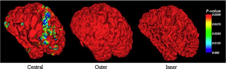
Fig. 10 shows the atrophy detection results for the central, inner, and outer cortical surface representation based methods respectively. For the case of 80% GM shrinkage, all of the three surface representation methods successfully detected most of the regions with simulated shrinkages, as shown in Fig. 10a. For the case of 40% shrinkage, apparently, the central cortical surface-based GM representation successfully detected a large percentage of the areas of simulated atrophy, but the inner and outer cortical surface based representation methods failed to do so, as shown in Fig. 10b. The result in Fig. 10 demonstrates that the central cortical surface representation of GM has superiority over the inner and outer cortical surface representations in detecting brain atrophy.

Fig. 10.

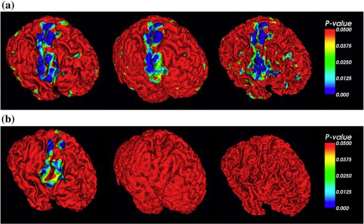
Detected brain atrophy using the measurement of GM density. P-values larger than 0.05 are coded by red (without statistical correction). The color bar is on the right. The left column is the central surface, the middle column is the outer surface, and the right column is the inner surface. (a). 80% shrinkage. (b). 40% shrinkage.

The measurement of GM thickness (MacDonald et al., 2000) is also adopted to detect the simulated brain atrophy. The GM thickness defined on each vertex of the three cortical surfaces in our experiment is the path length along the normal direction of each vertex within the GM. For the vertex on the inner/outer surface, the thickness is defined as the length from the inner/outer surface vertex to the outer/inner surface along the normal direction on the inner/outer surface vertex. For the vertex on central surface, the thickness is defined as the length from the inner surface to the outer surface vertex along the normal direction on the central surface vertex. The detection result of using 40% shrinkage is shown in Fig. 11, which also demonstrates that the central cortical surface has superiority over the inner and outer cortical surface in brain atrophy detection.

Fig. 11.

Detected brain atrophy using the measurement of GM thickness.

Discussion and conclusion

The proposed EDT method has been compared with the GVF method, the GGVF method, and the method implemented in FreeSurfer using synthesized images and real images. However, in this paper, the comparison measures are limited to the surface distance or non-GM percentage. More comparison measures are needed in the future for extensive comparison on larger datasets. Notably, it takes a couple of hours to reconstruct the central surface from segmented image in FreeSurfer. Both GVF and EDT methods take around 10 min, whereas the GGVF method takes around 10−20 min to converge.

It has been shown that the central cortical surface representation performs better than the inner and outer cortical surface representations in the detection of simulated GM shrinkage. Notably, the t statistic results on the surface in this paper are not corrected by the multiple statistics correction. Our future work will investigate the multiple comparison correction method based on statistical flattening (Worsley et al., 1999; Andrade et al., 2001). It is evident in Fig. 10 that there are significant regions (P-value<0.05) outside of the simulated atrophy areas for the case of 80% shrinkage (Fig. 10a) while there are no such unexpected significant regions for the 40% shrinkage. One possible explanation is that larger simulated atrophy and the induced deformation in the whole brain in the case of 80% shrinkage result in more errors in the hybrid volumetric and surface warping procedure than those in the case of 40% shrinkage. Those errors might cause the random noises in the significance detection in Fig. 10a, this issue will be investigated in our future work. In the future, we will also investigate what is the shrinkage limit, e.g., 20% or 10% shrinkage, of these methods to detect the simulated atrophies successfully.

As the reconstructed central surface better captures the geometric information of the entire cortex than the inner or outer cortical surfaces, it might be applied to a variety of surface-based structural and functional analysis of the human brain. For example, the central cortical surface representation can be used for surface-based brain registration (Liu et al., 2004). Measures such as GM density, cortical thickness, asymmetry (Thompson et al., 2004), diffusivity (Liu et al., 2006), and many other functional attributes (Park et al., 2006), can be mapped to the central cortical surface for group analysis. The f MRI activities can also be mapped onto central cortical surfaces for surface-based activation detection (Andrade et al., 2001). It should be noted that the potential advantages of central surface representation is that it has better geometric representation of the cortex. If the measurement index is related to geometry of the cortex, e.g., gray matter density, the central surface representation possibly has advantages. However, the central surface representation would not have advantage over the inner or outer surface representations if the features are not related to geometric information.

In summary, this paper presents a novel method that uses the EDT vector field as an external force in the deformable surface model to reconstruct the central surface from MRI brain images. Both real image data and simulated brain cortex images have been used to demonstrate the performance of the proposed method, as well as its comparisons with the other two methods. In particular, the reconstructed central cortical surface representation was applied to detect simulated GM shrinkages and showed better performance than the inner and outer cortical surface representations.

References

- Andrade A, Kherif F, Mangin JF, Worsley K, Paradis AL, Simon O, Dehaene S, Poline JB. Detection of f MRI activation using cortical surface mapping. Hum. Brain Mapp. 2001;12:79–93. doi: 10.1002/1097-0193(200102)12:2<79::AID-HBM1005>3.0.CO;2-I. [DOI] [PMC free article] [PubMed] [Google Scholar]
- Abrams L, Fishkind DE, Priebe CE. A proof of the spherical homeomorphism conjecture for surfaces. IEEE Trans. Med. Imag. 2002;21(12):1564–1566. doi: 10.1109/TMI.2002.806590. [DOI] [PubMed] [Google Scholar]
- Chung MK, Robbins SM, Dalton KM, Davidson RJ, Alexander AL, Evans AC. Cortical thickness analysis in autism with heat kernel smoothing. NeuroImage. 2005;25(4):1256–1265. doi: 10.1016/j.neuroimage.2004.12.052. [DOI] [PubMed] [Google Scholar]
- Cohen LD. On active contour models and balloons. CVGIP, Image Underst. 1991;53(2):211–218. [Google Scholar]
- Dale AM, Fischl B, Sereno MI. Cortical Surface-Based Analysis I: Segmentation and Surface Reconstruction. NeuroImage. 1999;9(2):179–194. doi: 10.1006/nimg.1998.0395. [DOI] [PubMed] [Google Scholar]
- Drury HA, Van Essen DC, Anderson CH, Lee CW, Coogan TA, Lewis JW. Computerized mappings of the cerebral cortex: a multiresolution flattening method and a surface-based coordinate system. J. Cogn. Neurosci. 1996;8(1):1–28. doi: 10.1162/jocn.1996.8.1.1. [DOI] [PubMed] [Google Scholar]
- Davatzikos C, Bryan RN. Using a deformable surface model to obtain a shape representation of the cortex. IEEE Trans. Med. Imag. 1996;15:785–795. doi: 10.1109/42.544496. [DOI] [PubMed] [Google Scholar]
- Davatzikos C, Prince JL, Bryan RN. Image registration based on boundary mapping. IEEE Trans. Med. Imag. 1996;15(1):112–115. doi: 10.1109/42.481446. [DOI] [PubMed] [Google Scholar]
- Fischl B, Dale AM. Measuring the Thickness of the Human Cerebral Cortex from Magnetic Resonance Images. Proc. Natl. Acad. Sci. 2000;97:11044–11049. doi: 10.1073/pnas.200033797. [DOI] [PMC free article] [PubMed] [Google Scholar]
- Fischl B, Salat DH, Busa E, Albert M, Dieterich M, Haselgrove C, van der Kouwe A, Killiany R, Kennedy D, Klaveness S, Montillo A, Makris N, Rosen B, Dale AM. Whole brain segmentation: automated labeling of neuroanatomical structures in the human brain. Neuron 31. 2002;33(3):341–355. doi: 10.1016/s0896-6273(02)00569-x. [DOI] [PubMed] [Google Scholar]
- Fischl B, Sereno MI, Dale AM. Cortical surface-based analysis II: inflation, flattening and a surface-based coordinate system. Neuro-Image. 1999;9:195–207. doi: 10.1006/nimg.1998.0396. [DOI] [PubMed] [Google Scholar]
- Gurtin ME. An introduction to continum mechanics. Academic Press; Orlando: 1981. [Google Scholar]
- Han X, Xu C, Prince JL. A topology preserving level set method for geometric deformable models. IEEE Trans. Pattern Anal. Mach. Intell. 2003;25(6):755–768. [Google Scholar]
- Jones SE, Buchbinder BR, Aharon I. Three-dimensional. mapping of cortical thickness using Laplace's equation. Hum. Brain Mapp. 2000;11(1):12–32. doi: 10.1002/1097-0193(200009)11:1<12::AID-HBM20>3.0.CO;2-K. [DOI] [PMC free article] [PubMed] [Google Scholar]
- Karacali B, Davatzikos C. Simulation of tissue atrophy using a topology preserving transformation model. IEEE Trans. Med. Imag. 2006;25(5):649–652. doi: 10.1109/TMI.2006.873221. [DOI] [PubMed] [Google Scholar]
- Kass M, Witkin A, Terzopoulos D. Snakes: active contour models. Int. J. Comput. Vis. 1987;1:321–331. [Google Scholar]
- Kim JS, Singh V, Lee JK, Lerch J, Ad-Dab'bagh Y, MacDonald D, Lee JM, Kim SI, Evans AC. Automated 3-D extraction and evaluation of the inner and outer cortical surfaces using a Laplacian map and partial volume effect classification. NeuroImage. 2005;27(1):210–221. doi: 10.1016/j.neuroimage.2005.03.036. [DOI] [PubMed] [Google Scholar]
- Kong TY, Rosenfeld A. Digital topology: introduction and survey. Comput. Vis. Graph. Image Process. 1989;48:357–393. [Google Scholar]
- Kwan RKS, Evans AC, Pike GB. MRI simulation-based evaluation of image-processing and classification methods. IEEE Trans. Med. Imag. 1999;18(11):1085–1097. doi: 10.1109/42.816072. [DOI] [PubMed] [Google Scholar]
- Liu T, Young G, Huang L, Chen N, Wong S. 76-space analysis of grey matter diffusivity: methods and applications. NeuroImage. 2006;15, 31(1):51–65. doi: 10.1016/j.neuroimage.2005.11.041. [DOI] [PubMed] [Google Scholar]
- Liu T, Shen D, Davatzikos C. Deformable registration of cortical structures via hybrid volumetric and surface warping. NeuroImage. 2004;22(Issue 4) doi: 10.1016/j.neuroimage.2004.04.020. [DOI] [PubMed] [Google Scholar]
- Lorensen WE, Cline HE. Marching cubes: A high-resolution 3-D surface construction algorithm. ACM Comput. Graph. 1987;21(4):163–170. [Google Scholar]
- Mangin JF, Frouin V, Bloch I, Regis J, Lopez-Krahe J. From 3-D magnetic resonance images to structural representations of the cortex topography using topology preserving deformations. J. Math. Imaging Vis. 1995;5(5):297–318. [Google Scholar]
- MacDonald D, Kabsni N, Avis D, Evans AC. Automated 3-D extraction of inner and outer surfaces of cerebral cortex from MRI. NeuroImage. 2000;12:340–355. doi: 10.1006/nimg.1999.0534. [DOI] [PubMed] [Google Scholar]
- McInerney T, Terzopoulos D. Deformable models in medical image analysis: a survey. Med. Image Anal. 1996;1(2):91–108. doi: 10.1016/s1361-8415(96)80007-7. [DOI] [PubMed] [Google Scholar]
- Miller MI. Computational anatomy: shape, growth, and atrophy comparison via diffeomorphisms. NeuroImage. 2004;23:S19–S33. doi: 10.1016/j.neuroimage.2004.07.021. [DOI] [PubMed] [Google Scholar]
- Miller MI, Massie AB, Ratnanather JT, Botteron KN, Csernansky JG. Bayesian Construction of Geometrically Based Cortical Thickness Metrics. NeuroImage. 2000;12(6):676–687. doi: 10.1006/nimg.2000.0666. [DOI] [PubMed] [Google Scholar]
- Montani C, Scateni R, Scopigno R. Discretized marching cubes. Proc IEEE. Visualization. 1994;94:281–287. [Google Scholar]
- Park HJ, Lee JD, Chun JW, Seok JH, Yun M, Oh MK, Kim JJ. Cortical surface-based analysis of 18F-FDG PET: measured metabolic abnormalities in schizophrenia are affected by cortical structural abnormalities. Neuroimage. 2006;31(4):1434–1444. doi: 10.1016/j.neuroimage.2006.02.001. [DOI] [PubMed] [Google Scholar]
- Sandor S, Leahy R. Surface-based labeling of cortical anatomy using a deformable atlas. IEEE Trans. Med. Imag. 1997;16:41–54. doi: 10.1109/42.552054. [DOI] [PubMed] [Google Scholar]
- Shattuck DW, Leahy RM. BrainSuite: an automated cortical surface identification tool. Med. Image Anal. 2002;6:129–142. doi: 10.1016/s1361-8415(02)00054-3. [DOI] [PubMed] [Google Scholar]
- Shattuck DW, Leahy RM. Automated graph-based analysis and correction of cortical volume topology. IEEE Trans. Med. Imag. 2001;20(11):1167–1177. doi: 10.1109/42.963819. [DOI] [PubMed] [Google Scholar]
- Thompson PM, Lee AD, Dutton RA, Geaga JA, Hayashi KM, Eckert MA, Bellugi U, Galaburda AM, Korenberg JR, Mills DL, Toga AW, Reiss AL. Abnormal Cortical Complexity and Thickness Profiles Mapped in Williams Syndrome. J. Neurosci. 2005;25(16):4146–4158. doi: 10.1523/JNEUROSCI.0165-05.2005. [DOI] [PMC free article] [PubMed] [Google Scholar]
- Thompson PM, Hayashi KM, Sowell ER, Gogtay N, Giedd JN, Rapoport JL, de Zubicaray GI, Janke AL, Rose SE, Semple J, Doddrell DM, Wang YL, van Erp TGM, Cannon TD, Toga AW. Mapping cortical change in Alzheimer's disease, brain development, and Schizophrenia. Neuroimage. 2004;23:S2–S18. doi: 10.1016/j.neuroimage.2004.07.071. [DOI] [PubMed] [Google Scholar]
- Thompson PM, Hayashi KM, de Zubicaray G, Janke AL, Rose SE, Semple J, Hong MS, Herman D, Gravano D, Dittmer S, Doddrell DM, Toga AW. Dynamics of Gray Matter Loss in Alzheimer's Disease. J. Neurosci. 2003;23(3):994–1005. doi: 10.1523/JNEUROSCI.23-03-00994.2003. [DOI] [PMC free article] [PubMed] [Google Scholar]
- Van Essen DC, Maunsell JHR. Two-dimensional maps of the cerebral cortex. J. Comput. Neurol. 1980;191:255–281. doi: 10.1002/cne.901910208. [DOI] [PubMed] [Google Scholar]
- Van Essen DC, Drury HA, Dickson J, Harwell J, Hanlon D, Anderson CH. An integrated software suite for surface-based analyses of cerebral cortex. J. Am. Med. Inform. Assoc. 2001;8:443–459. doi: 10.1136/jamia.2001.0080443. [DOI] [PMC free article] [PubMed] [Google Scholar]
- Worsley KJ, Andermann M, Koulis T, MacDonald D, Evans AC. Detecting changes in non-isotropic images. Hum. Brain Mapp. 1999;8:98–101. doi: 10.1002/(SICI)1097-0193(1999)8:2/3<98::AID-HBM5>3.0.CO;2-F. [DOI] [PMC free article] [PubMed] [Google Scholar]
- Xu C. PhD dissertation. Johns Hopkins University; 1999. Deformable models with application to human cerebral cortex reconstruction from magnetic resonance images. [Google Scholar]
- Xu C, Prince JL. Snakes, shapes, and gradient vector flow. IEEE Trans. Imag. Process. 1998;7:359–369. doi: 10.1109/83.661186. [DOI] [PubMed] [Google Scholar]
- Xu C, Pham DL, Pettmann ME, Yu DN, Prince JL. Reconstruction of the human cerebral cortex from magnetic resonance images. IEEE Trans. Med. Imag. 1999;18(6):467–480. doi: 10.1109/42.781013. [DOI] [PubMed] [Google Scholar]
- Xu MH, Thompson PM, Toga AW. Adaptive Reproducing Kernel Particle Method for Extraction of the Cortical Surface. IEEE Trans. Med. Imag. 2006;25(6):1–13. doi: 10.1109/tmi.2006.873614. [DOI] [PubMed] [Google Scholar]
- Zeng X, Staib LH, Schultz RT, Duncan JS. Segmentation and measurement of the cortex from 3D MR images. MICCAI. 1998:519–530. [Google Scholar]