Generalized Self-Consistency: Multinomial logit model and Poisson likelihood

Abstract

A generalized self-consistency approach to maximum likelihood estimation (MLE) and model building was developed in (Tsodikov, 2003) and applied to a survival analysis problem. We extend the framework to obtain second-order results such as information matrix and properties of the variance. Multinomial model motivates the paper and is used throughout as an example. Computational challenges with the multinomial likelihood motivated Baker (1994) to develop the Multinomial-Poisson (MP) transformation for a large variety of regression models with multinomial likelihood kernel. Multinomial regression is transformed into a Poisson regression at the cost of augmenting model parameters and restricting the problem to discrete covariates. Imposing normalization restrictions by means of Lagrange multipliers (Lang, 1996) justifies the approach. Using the self-consistency framework we develop an alternative solution to multinomial model fitting that does not require augmenting parameters while allowing for a Poisson likelihood and arbitrary covariate structures. Normalization restrictions are imposed by averaging over artificial “missing data” (fake mixture). Lack of probabilistic interpretation at the “complete-data” level makes the use of the generalized self-consistency machinery essential.

1 Introduction

MP transformation has been a popular technique to simplify maximum like­lihood estimation and the derivation of the information matrix in a variety of models yielding multinomial likelihoods Baker (1994). The approach works by substituting a Poisson likelihood for the multinomial likelihood at the cost of augmenting the model parameters by auxillary ones.

Multimonial probabilities p_i(z), i = 1,…, K are modeled using log-linear predictors θ_i(z) specific to categories i and conditional on a vector of covari-ates z. Multinomial logit model is constructed by normalization

$$p_i\left(z\right)=\frac{{\theta }_i\left(z\right)}{\underset{k=1}{\overset{K}{\Sigma }}{\theta }_k\left(z\right)},$$ (1)

where without loss of generality θ₁ is restricted to 1 for identifiability.

Each θ_i can be parameterized using a vector of regression coefficients β_i so that

$${\theta }_i\left(z\right)=\exp \left\{{\beta }_i^{\mathrm{T}}z\right\}.$$ (2)

Data can be represented as a set {y_ij, z_j}, i = 1,…, K, j = 1,…, N, where y_ij = 1 if observation j with covariates zj falls into category i, and y_ij = 0, otherwise.

The log-likelihood kernel corresponding to the above formulation can be written as

$${\ell }_{\mathrm{M}}=\underset{\mathit{ij}}{\Sigma }{y}_{\mathit{ij}}\left\{\log \left({\theta }_{\mathit{ij}}\right)-\log \left[\underset{k=1}{\overset{K}{\Sigma }}{\theta }_{\mathit{kj}}\right]\right\},$$ (3)

where θ_ij = θ_i(z_j).

With categorical covariates z summarized into groups, y_ij becomes a count of observations in response category i belonging to group j. We may then index the predictors by the group as θ_ij so that expression (3) retains its form with this understanding, and with N in this case being the number of groups rather than subjects.

The parameters in the model form a potentially large matrix B = [β_ij], which may create computational problems. Baker (1994) argued that computations can be simplified by maximizing a Poisson likelihood

$${\ell }_{\mathrm{MP}}=\underset{\mathit{ij}}{\Sigma }\left\{y_{\mathit{ij}}\log \left(e^{{\varphi }_j}{\theta }_{\mathit{ij}}\right)-e^{{\varphi }_j}{\theta }_{\mathit{ij}}\right\},$$ (4)

in the discrete covariate situation, where ϕ_j, j = 1,…, N are auxillary variables augmenting the model parameters. It can be shown that ℓ_M is indeed a profile likelihood for ℓ_MP as ϕs are maximized out.

Many other models lend themselves naturally to the MP approach such as repeated categorical measurements (Conaway, 1992), capture-recapture models (Cormack, 1990), log-linear models (Palmgren, 1981), Rasch models (Tiur, 1982), and Proportional Hazards model (Whitehead, 1980), to name a few. Recently, there has been a surge in Bayesian applications of the methodology (Ghosh et al., 2006).

The MP transformation can be justified through the method of Lagrange multipliers (Lang, 1996). To do so one can consider the model for group j and category i in the form p_ij = θ_0jθ_ij, where the variables θ_0j are meant to be determined to satisfy the normalization restriction

$$\underset{\mathit{i}}{\Sigma }{p}_{\mathit{ij}}=1,j=1,\dots ,N,\text{or}{\phi }_j=1-\underset{\mathit{i}}{\Sigma }{\theta }_{0j}{\theta }_{\mathit{ij}}=0.$$ (5)

It can be shown that the optimal value of the Lagrange multiplier λ_j in the penalized multinomial likelihood

$${\ell }_{\mathrm{LM}}=\underset{\mathit{ij}}{\Sigma }{y}_{\mathit{ij}}\log \left(p_{\mathit{ij}}\right)+\underset{j}{\Sigma }{\lambda }_j{\phi }_j$$

is ${\widehat{\lambda }}_j={\Sigma }_i{y}_{\mathit{ij}}$, and that the kernel of ${\ell }_{\mathrm{LM}}\left(\widehat{\lambda }\right)$ is ℓ_MP with

$${\varphi }_j=\log \left({\theta }_{0j}{\widehat{\lambda }}_j\right).$$

Solving for ϕ_j is equivalent to enforcing the normalization restriction (5). It is now clear that normalization needs to be enforced for each distinct value of z, hence one parameter ϕ is spent per each such value. The MP approach outlined above has two major limitations:

• The approach is limited to categorical covariates;

• The approach inflates the model dimension that can already be high if B = [β_ij] is a large matrix, adding to potential computational difficulties associated with the matrix inverse.

The above two limitations are addressed in this paper as an example of an application of the generalized self-consistency approach Tsodikov (2003). We will present a procedure that solves K − 1 Poisson regressions each with only a subset β_i of parameters in a nested EM-like iterative algorithm.

2 Fake Mixture

Let p(x | z) be a family of probability distributions describing a model for the random response X regressed on covariates z. In the case of multinomial likelihood, x will be a discrete variable pointing at categories.

The idea of the fake mixture is to artificially represent p(x | z) as a mixture model

$$p(x\mid \mathit{z})=\mathrm{E}\left\{p(x\mid \mathit{z},U)\right\},$$ (6)

where U is a mixing variable representing artificial missing data, and p(·|·, U) are some complete-data probabilities conditional on U. In other words, a fake mixture model is considered such that one gets the original target model when missing data are integrated out.

In the multinomial case considered in this paper we are looking for a fake mixture formulation such that p on the left of (6) corresponds to the multinomial distribution, while the p on the right of (6) yields Poisson complete–data likelihood. Once a fake mixture transformation is defined, we can construct an EM algorithm with E-step soving the problem of imputation of U, while M-step dealing with maximizing a log-likelihood obtained from the complete–data model p(x | z, U).

Observe that the Laplace transform of an exponentially distributed random variable U ∝ Exp(1) with expectation of 1 has the form

$$\mathcal{L}\left(s\right)=\mathrm{E}\left\{e^{-Us}\right\}=\frac{1}{1+s}.$$ (7)

Therefore, noting that θ₁ = 1, the multinomial probabilities (1) can be written in the fake mixture form

$$p_i\left(\mathit{z}\right)={\theta }_i\left(\mathit{z}\right)\mathrm{E}\left\{\exp \left[-U\underset{k=2}{\overset{K}{\Sigma }}{\theta }_k\left(\mathit{z}\right)\right]\right\},$$ (8)

with p(·|·, U) obtained by dropping the “E” symbol from the above expression

$$p_i(\mathit{z}\mid U)={\theta }_i\left(\mathit{z}\right)e^{-U\underset{k=2}{\overset{K}{\Sigma }}{\theta }_k\left(\mathit{z}\right)}.$$ (9)

Formally, (9) gives rise to a sum of Poisson complete–data log-likelihoods parameterized in a disjoint fashion

$${\ell }_{\mathrm{CD}}\left(\mathit{B}\right)=\underset{i=1}{\overset{K}{\Sigma }}\underset{j=1}{\overset{N}{\Sigma }}\log \left\{p_i({\mathit{z}}_j\mid U_j)\right\}=\underset{i=2}{\overset{K}{\Sigma }}{\ell }_{\mathrm{CD},i}\left({\beta }_i\right),$$ (10)

where i goes over categories and j goes over subjects, and

$${\ell }_{\mathrm{CD},i}=\underset{j=1}{\overset{N}{\Sigma }}\{y_{\mathit{ij}}\log \left({\theta }_{\mathit{ij}}\right)-y_{\ast j}{U}_j{\theta }_{\mathit{ij}}\}$$ (11)

is a Poisson likelihood specific to the ith category parameterized by β_i, the vector represented by the transposed ith row of the parameter matrix B. Note that we used the identifiability restriction θ₁ = 1 in the derivation of (10) that resulted in the summation over i starting at i = 2. The term y_*j = Σ_i y_ij is equal to one if j has the meaning of subjects. In the discrete formulation where j refers to a group of subjects with a common covariate vector, y_*j is the count of subjects in group j.

With a suitably imputed $U_j\to {\widehat{U}}_j$, maximizing (11) with respect to β_i as a standard Poisson GLM would constitute the M-step of the algorithm.

However, on closer examination of the above formulation we are faced with the following difficulty. The complete–data “probabilities” (9) are not really probabilities and do not correspond to any probabilistic model on the complete–data level (It suffices to note that p_i(·|·, U) have the range of (0,∞)). Imputation in the EM algorithm is defined through a conditional expectation operator applied to the complete–data loglikelihood given observed data. Without the complete–data model making probabilistic sense, it is not immediately clear how the conditional expectation given observed data and imputation can be defined, let alone whether the properties of the EM algorithm will be preserved.

Note that if complete-data model were a legitimate probability model, ℓ_CD would be a conditional log-likelihood given missing data U based on that model. With ℓ_CD kernel being linear in U, the imputation at the E-step would reduce to taking conditional expectation of U given observed data, which can be written as

$$\widehat{U}=\mathrm{E}\{U\mid \text{Observed data}\}=\frac{\mathrm{E}\left\{U{L}_{\mathrm{CD}}\left(U\right)\right\}}{\mathrm{E}\left\{L_{\mathrm{CD}}\left(U\right)\right\}},L=\exp \left(\ell \right).$$ (12)

It can be shown that (12) holds its validity as the E-step of an EM-like algorithm when ℓ_CD does not correspond to a valid probabilistic model, as in the case considered in this paper. Justification of the above statement and a derivation of a ready-to-use form of (12) would repeat the one for a more general Quasi-Expectation operator introduced in (Tsodikov, 2003). Therefore, we will simply refer to the properties of the QE operator reviewed in the next section and get Û and monotonicity result for the corresponding QEM algorithm immediately as a corollary.

3 The Quasi-Expectation Operator

Probabilities that define a marginal mixed model (6) can be viewed as an integral transform of the distribution of missing data. As an example, the mixed form (8) is defined through the Laplace transform (7) of missing data variable U. It is well known that derivatives of a Laplace transform ℒ(s) = E {e^−Us} can be used to find moments of the corresponding random variable as well as expectations of the form E {U^ke^−Us} by taking derivatives of the transform with respect to s Oftentimes, conditional expectation of U given observed data used at the E-step can be expressed through the expectations just mentioned. If this is the case, E-step is easily constructed using a few derivatives of ℒ(s) without invoking integration using the distribution of missing data. This means that a particular EM can be defined using a few conditional moments of U rather than the full distribution (that is defined using all conditional moments of order k = 0, 1,…,∞ by the inversion theorems for the Laplace transform). This observation paves the road to generalizing EMs so that only a finite set of derivatives of the model distribution such as (8) with respect to model parameters are required to behave like a real mixed model would, for the algorithm to work. We call such algorithms Quasi-EM (QEM).

Imputation and the QEM construction is based on the quasi-expectation operator QE defined in (Tsodikov, 2003). Let e_i(u, s) be some basis functions, where u is an argument of the function, and s is a parameter. We shall follow the rule that integral operators like E act on e as a function of u, while differential operators will act on e as a function of s, i.e. derivatives will be with respect to s unless noted otherwise. This convention follows the basic idea of integral transforms that replace the problem in the space of functions of u equipped with an integral operator by the one of s equipped with a differential operator.

For the purposes of this paper it is sufficient to consider a set of three basis functions generating the space of admissible functions as a linear span.

$$e_0(u,s)=e^{-\mathit{us}},e_1(u,s)={\mathit{ue}}^{-\mathit{us}},\text{and}{e}_2(u,s)=u^2{e}^{-\mathit{us}}.$$ (13)

This is the same set that was used to derive efficient numerical algorithms for semiparametric survival models in (Tsodikov, 2003). The basis functions are chosen based on the following properties

• A linear span of the basis functions with appropriately chosen parameter s includes the complete–data model (9), complete–data likelihood and log-likelihood (11) and, as we will see later, arguments of the imputation operator.

• The kernel that depends on s is log-linear in u. As model parameters will enter the formulation through s, this yields a complete–data log-likelihood kernel that is linear in u. This reduces the E-Step to the imputation of u by a conditional QE.

• Next function is a consequence of the derivative of the previous

  $$e_{k+1}={\mathit{ke}}_{k-1}-e_k^{\prime },$$ (14)

  where here and below equalities are functional (uniform with respect to the argument). This ensures that such functions can be cloned based on specifying the first one and generating the others recurrently by differentiation. Also, this ensures that the values of the QE on basis functions can be cloned in a similar fashion.

QE is defined as a linear operator on the linear span of {e_k} such that

$$\mathrm{QE}\left\{e_1\left(s\right)\right\}=\gamma \left(x\right),x=e^{-s}$$ (15)

$$\frac{\partial }{\partial s}\mathrm{QE}\left\{e_k\left(s\right)\right\}=\mathrm{QE}\left\{\frac{\partial }{\partial s}{e}_k\left(s\right)\right\}$$ (16)

The function γ(x) is called a model generating function. There are two reasons behind the name. Firstly, note that if QE is an expectation, then QE(e₁) is a Laplace transform ℒ(s) if considered as a function of s, and a probability generating function of U, γ(x), when considered as a function of x = exp(−s). And secondly, as follows from (15), (16) and (14), values of QE on any basis function are derived recurrently by differentiating γ.

Finally, for any functions f, g, and fg in the {e_k} linear span, conditional QE is defined as

$$\mathrm{QE}\{f\mid g\}=\frac{\mathrm{QE}\left\{\mathit{fg}\right\}}{\mathrm{QE}\left\{g\right\}}.$$ (17)

The QEM algorithm is a procedure designed to maximize a likelihood of the form

$$L\left(\beta \right)=\mathrm{QE}\left\{L_{\mathrm{CD}}(\beta \mid u)\right\},$$ (18)

where L_CD(β|u), as a function of u, is admissible (belongs to the linear span of the basis functions that define the QE). The following recurrent expression defines the procedure.

$${\beta }^{(m+1)}=\underset{\beta }{\arg \max \mathrm{QE}}\left\{\log L_{\mathrm{CD}}(\beta \mid u)\mid L_{\mathrm{CD}}({\beta }^{\left(m\right)}\mid u)\right\},$$ (19)

where all the arguments of the conditional QE are supposed to be admissible.

When log L_CD(β|u) is linear in u, the imputation is reduced to taking a conditional QE (17) with f = u and g = L_CD(u) (compare with (12)). The QEM algorithm was shown to be monotonic when QE is Jensen–compliant, that is

$$\mathrm{QE}\{\log \left(f\right)\mid g\}<\log \left[\mathrm{QE}\{f\mid g\}\right].$$ (20)

It was also shown that in order for (20) to hold, it is sufficient that conditional QEs of the form

$$\Theta (x\mid c)=\mathrm{QE}\{u\mid e_c\left(s\right)\},c=0,1;x=e^{-s}$$ (21)

represent non-increasing functions of s (non-decreasing functions of x). This is the case whenever QE operators in the right side of (17) are expectations (shown in (Tsodikov, 2003)) as in our case (12). In terms of the model-generating function γ the imputation operator Θ(x|c) assumes a ready-to-use general form (Tsodikov, 2003)

$$\Theta (x\mid c)=\mathrm{QE}\{u\mid u^c{x}^u\}=c+x\frac{{\gamma }^{(c+1)}\left(x\right)}{{\gamma }^{\left(c\right)}\left(x\right)},c=0,1,$$ (22)

where γ^(a) is the derivative of order a.

4 The Quasi-EM Algorithm for Multinomial Likelihood

Invoking the results reviewed in the previous section, let us now proceed with the QEM construction for the multinomial likelihood.

Motivated by (7) and (8), we choose the model generating function

$$\gamma \left(x\right)=\frac{1}{1-\log \left(x\right)}.$$ (23)

Note that the above γ represents a generating function also used for a Proportional Odds survival model (Tsodikov, 2003). We may write the multinomial model as

$$p_i\left(\mathit{z}\right)={\theta }_i\left(\mathit{z}\right)\gamma \left(x\right)=\mathrm{QE}\left\{{\theta }_i\left(\mathit{z}\right)e_0(u,s)\right\},x=e^{-s},s=\underset{k=2}{\overset{K}{\Sigma }}{\theta }_k\left(\mathit{z}\right).$$ (24)

Likelihood expressions (10) and (11) are without change. However, they are now consequences of (24) with U = u considered as the argument of a function as in (13), rather than a random variable.

Using (22) and the fact that complete-data likelihood only involves e₀ (24), the imputation operator is easily seen to be

$$\widehat{U}=\Theta (e^{-s}\mid 0)=\frac{1}{1+s},$$ (25)

where $s={\Sigma }_{k=2}^K{\theta }_k\left(z\right)$. The QEM algorithm is now formulated as follows.

1. Set initial values of regression coefficients ${\beta }_i^{\left(0\right)}$, i = 2,…,K. They can be zero-vectors to start with. This is iteration m = 0.

2. For each subject j compute

   $${\widehat{U}}_j^{\left(m\right)}=\frac{1}{1+s_j},$$ (26)

   where

   $$s_j=\underset{k=2}{\overset{K}{\Sigma }}{\theta }_{\mathit{kj}}^{\left(m\right)}\text{and}{\theta }_{\mathit{kj}}^{\left(m\right)}=\exp \left\{{\beta }_k^{\left(m\right)\mathrm{T}}{\mathit{z}}_j\right\}.$$ (27)
3. Solve K − 1 separate Poisson MLE problems

   $${\beta }_i^{(m+1)}=\arg \underset{{\beta }_i}{\max }\underset{j=1}{\overset{N}{\Sigma }}\left\{y_{\mathit{ij}}\log \left({\theta }_{\mathit{ij}}\right)-y_{\ast j}{\widehat{U}}_j^{\left(m\right)}{\theta }_{\mathit{ij}}\right\},$$ (28)

   i = 2,…,K, where ${\theta }_{\mathit{ij}}=\exp \left\{{\beta }_i^T{z}_j\right\}$.

4. Test convergence. Stop if convergence is reached. Otherwise, increment m and return to step 2.

As a QEM algorithm, the above procedure improves the likelihood at each step, works with only a subset β_j of parameters at a time, and does not use any matrix inverses. These properties guarantee convergence in likelihood (even when the model is overparameterized and non-identifiable) and impart the algorithm with great stability.

5 Variance Estimation

5.1 General results

Variance estimation with the EM algorithm is based on the so-called missing information principle representing the observed information

$$I=-\frac{{\partial }^2\ell \left(\beta \right)}{\partial \beta \partial {\beta }^{\mathrm{T}}}$$ (29)

as difference between complete-data information and missing information. A number of procedures have been proposed, (Louis, 1982) and (Oakes, 1999), to name a few. Previous derivations explicitly relied on expressions involving the conditional probability density of complete data given observed data. The tone of this paper so far has been to avoid this since our complete data MLE problem is fake and does not have a probability interpretation. Moreover, for some models with non-smooth derivatives of the model generating function of some order (ex. defined by splines), the mixture formulation (6) does not exist, let alone imputation by means of conditional expectation. We are therefore looking to derive a similar general result for models formulated using QE as in (18). Derived in Appendix 1 is the following generalized missing information principle. For any likelihood L(β) = QE{L_CD(β|u)},

$$I=\mathrm{QE}\left\{\phantom{\mid }{I}_{\mathrm{CD}}-\frac{\partial {\ell }_{\mathrm{CD}}}{\partial \beta }\frac{\partial {\ell }_{\mathrm{CD}}}{\partial {\beta }^{\mathrm{T}}}\mid L_{\mathrm{CD}}\right\},$$ (30)

where expressions are evaluated at the MLE $\beta =\widehat{\beta }$,

$$I_{\mathrm{CD}}=-\frac{{\partial }^2{\ell }_{\mathrm{CD}}(\beta \mid u)}{\partial \beta \partial {\beta }^{\mathrm{T}}}.$$

Here I = ℐ_CD − ℐ_MD, where ℐ_CD = QE{I_CD | L_CD} is the expected complete-data information, while ${\mathcal{I}}_{\mathrm{MD}}=\mathrm{QE}\left\{\phantom{\mid }\frac{\partial {\ell }_{\mathrm{CD}}}{\partial \beta }\frac{\partial {\ell }_{\mathrm{CD}}}{\partial {\beta }^{\mathrm{T}}}\mid L_{\mathrm{CD}}\right\}$ is the expected missing information.

The above statement like similar results in the EM literature is not helpful as far as computation of the information matrix is concerned unless it can be further specified for a particular class of models. The QE construction of Section 3 allows us to streamline the specification of the algorithm for a model (Section 4), as the imputation operator is readily expressed through derivatives of the model generating function resulting in a closed-form QE-step. Similar results will now be derived for the information matrix.

The form of the complete-data likelihood (11) motivates us to consider a class of models with L_CD of the form

$$L_{\mathrm{CD}}=\exp \{-A\left(\beta \right)u+B\left(\beta \right)\}.$$ (31)

Derived in Appendix 3 are the following expressions for the components of the observed information matrix based on (31)

$${\mathcal{I}}_{\mathrm{CD}}=\frac{{\partial }^{2}A}{\partial \beta \partial {\beta }^{\mathrm{T}}}\Theta (e^{-A}\mid 0)-\frac{{\partial }^{2}B}{\partial \beta \partial {\beta }^{\mathrm{T}}}$$ (32)

$${\mathcal{I}}_{\mathrm{MD}}=\frac{\partial A}{\partial \beta }\frac{\partial A}{\partial {\beta }^{\mathrm{T}}}\mathcal{V}\left(e^{-A}\right),$$ (33)

$$\mathcal{V}\left(x\right)=\Theta (x\mid 0)[\Theta (x\mid 1)-\Theta (x\mid 0)],$$ (34)

where Θ is given by (22).

The function Θ(e^−A|0) is a surrogate of conditional expectation of missing data U given observed data. To see this observe that the basis function e₀ = x^u that is used as a condition in

$$\Theta (x\mid 0)=\mathrm{QE}\{u\mid x^u\}=\mathrm{QE}\{u\mid {\mathit{ax}}^u\}$$ (35)

for any constant a, represents the complete-data likelihood (31) with x = e^−A, and a = e^B. To see the validity of the above interpretation we need to recall the definition of conditional QE (17), the fact that QE=E if U is a random variable, and the form of the conditional expectation of U given observed data given by (12). Finally, the interpretation would turn into reality if, additionally, L_CD(U) were a complete-data likelihood based on a probabilistically valid model. The latter is not the case with our treatment of the multinomial model as mentioned earlier.

Similarly, V can be interpreted as a surrogate of the conditional variance of U given observed data. Using the quasi-expectation operator, conditional quasi-variance QVar can be defined as

$$\mathrm{QVar}(f\mid g)=\mathrm{QE}(f^2\mid g)-{\mathrm{QE}}^2(f\mid g).$$

for admissible functions f(u) and g(u). Then, as shown in Appendix 2,

$$\mathcal{V}\left(x\right)=\mathrm{QVar}\{u\mid x^u\},$$ (36)

and the interpretation proceeds similar to that of Θ. Note that “missing information” I_MD is proportional to the conditional “variance of missing data” given observed data V.

Also, shown in the Appendix 2 is that

$$\frac{\partial \Theta (e^{-s}\mid 0)}{\partial s}=-\mathcal{V}\left(e^{-s}\right).$$ (37)

According to (37), non-descreasing character of the functions Θ (22) guarantees that QVar is non-negative, QE is Jensen-compliant (Tsodikov, 2003), Θ(· | 1) ≥ Θ(· | 0) (from (34)), the missing data information matrix (33) is non-negative definite, and that QEM iterations are performed by a contracting operator with matrix speed of convergence expressed by the missing information fraction ${\mathcal{I}}_{\mathrm{MD}}{\mathcal{I}}_{\mathrm{CD}}^{-1}$. This chain of facts triggered by the non-descreasing Θ assumption involving second order conditional “moments” of U determines the EM-like behavior of the QEM procedure.

5.2 Information matrix for the multinomial likelihood

The general results of the previous subsection allow us to derive the observed information matrix for the multinomial likelihood. Observe that the subject j contribution to the complete-data likelihood (10), (11) follows the general form (31). Explicitly,

$${\ell }_{\mathrm{CD}}=\log L_{\mathrm{CD}}=\underset{i=2}{\overset{K}{\Sigma }}\underset{j=1}{\overset{N}{\Sigma }}-A_{\mathit{ij}}{u}_j+B_{\mathit{ij}},$$ (38)

with A_ij = y_*jθ_ij, and B_ij = y_ij log θ_ij. Exponential parameterization of θ in terms of regression coefficients β yields linear B, hence ∂²B /∂β∂β^T = 0. Using this observation and the results (32), (33) of the previous section we get the observed information matrix for the multinomial model

$$I=\underset{j=1}{\overset{N}{\Sigma }}\frac{{\partial }^2{A}_{\ast j}}{\partial \beta \partial {\beta }^{\mathrm{T}}}\Theta (e^{-A_{\ast j}}\mid 0)-\frac{\partial A_{\ast j}}{\partial \beta }\frac{\partial A_{\ast j}}{\partial {\beta }^{\mathrm{T}}}\mathcal{V}\left(e^{-A_{\ast j}}\right),$$ (39)

where A_*j = Σ_iA_ij. In the above expression β is thought of as being a block-vector of regression coefficients with blocks corresponding to vectors β_i specific to categories i = 2,…, K. Using (22) with c = 1, we have

$$\Theta (e^{-s}\mid 1)=\frac{2}{1+s},$$ (40)

which together with (25) and (34) gives

$$\Theta (e^{-A_{\ast j}}\mid 0)=\frac{1}{1+A_{\ast j}};\mathcal{V}\left(e^{-A_{\ast j}}\right)=\frac{1}{{(1+A_{\ast j})}^2}.$$ (41)

Finally, specification of the information matrix is completed by taking the derivatives of A with respect to β

$$\frac{{\partial }^2{A}_{\ast j}}{\partial \beta \partial {\beta }^{\mathrm{T}}}=\text{block-diag}\left({\theta }_{\mathit{ij}}{z}_j{z}_j^{\mathrm{T}}\right),$$

where the diagonal (K – 1) × (K – 1) block-matrix is built using dim(z) × dim(z) blocks indexed by i = 2,…, K, and where the (K – 1) × (K – 1) block-matrix T_j is composed of dim(z) × dim(z) blocks ${\mathit{T}}_{\mathit{jab}}=z_j{z}_j^{\mathrm{T}}{\theta }_{\mathit{aj}}{\theta }_{\mathit{bj}}$, a = 2,…, K, b = 2,…,K.

7 Simulation Study

In this section, we study the QEM algorithm by simulations. The results will be compared with the Newton-Raphson algorithm traditionally used to fit the model.

We consider a multinomial response with four categories regressed on three covariates. The covariates are generated from standard normal distribution with one of the covariates dichotomized using a cutpoint at zero. Parameter values used to simulate the data are shown in Table 1.

Table 1.

Empirical means of parameter estimates obtained by the QEM algorithm based on 10,000 simulated replicates

	True parameter values			Empirical mean
	Contrasts			Contrasts
Variables	2 vs. 1	3 vs. 1	4 vs. 1	2 vs. 1	3 vs. 1	4 vs. 1
Intercept	−0.60	−0.30	−1.00	−0.61	−0.30	−1.01
z1	−0.80	0.70	2.10	−0.81	0.71	2.12
z2	−1.00	−0.10	−0.10	−1.01	−0.10	−0.10
z3	−2.00	0.10	1.00	−2.03	0.10	1.01

We generated 10,000 datasets each of size 1000 and fitted the model to each dataset. Empirical estimates of the mean of point estimates agree well with the true parameter values as presented in Tables 1.

Shown in Table 2 are the corresponding standard errors. Note a good agreement of empirical estimates of standard errors (“S²”) from 10,000 replicates of point estimates of regression coefficients and the empirical mean of standard errors based on the observed information matrix I⁻¹ (30). To illustrate the missing information principle we also computed standard errors based on the complete data information matrix (32) as if U were observed. It is evident that complete-data standard errors that ignore uncertainty associated with “missing data” are consistently smaller than the ones based on observed data just as one would expect it to be in a real missing data problem.

Table 2.

Standard errors (STE) of parameter estimates obtained by the QEM algorithm based on 10,000 simulated replicates. “S²” corresponds to an empirical sum of squares estimate of variance based on a sample of point estimates of respective regression coefficients. Other types of STE estimators are based on inverted information matrices I⁻¹ and ${\mathcal{I}}_{\mathrm{CD}}^{-1}$.

	Contrasts
Variables	2 vs. 1			3 vs. 1			4 vs. 1
	S2	I−1	${\mathcal{I}}_{\mathrm{CD}}^{-1}$	S2	I−1	${\mathcal{I}}_{\mathrm{CD}}^{-1}$	S2	I−1	${\mathcal{I}}_{\mathrm{CD}}^{-1}$
Intercept	0.16	0.15	0.12	0.14	0.13	0.10	0.17	0.17	0.12
z1	0.14	0.14	0.10	0.12	0.12	0.09	0.15	0.15	0.07
z2	0.13	0.13	0.08	0.10	0.10	0.07	0.10	0.10	0.06
z3	0.27	0.26	0.21	0.19	0.19	0.14	0.21	0.21	0.12

One of the advantages of the QEM algorithm's performance is its stability. There are a number of reasons for the stable behavior of the algorithm.

1. The original problem involving a matrix of parameters representing both caterories of response and covariates for each category is broken down into a set of separate Poisson regression problems each of the dimension of the covariate vector only. That is, we have a factorization by categories at the M-step.

2. No matrix inverses are involved in maximization of the likelihood.

3. The algorithm would not even be deranged by a non-identifiable problem and would return one solution out of a set of possible solutions with the same maximal likelihood value.

To illustrate the above points we applied the QEM algorithm to a sparse problem. Sparse data are created with n = 100 observations in each dataset. The model has four response categories and one binary covariate. Parameter values for the intercept term and for the binary covariate used to simulate data are shown in Table 4 and are deliberately chosen to make category 3 sparse as shown in Table 3. We generated 10,000 datasets and fitted the multinomial logit model to the sparse data using QEM and Newton Raphson algorithms. Descriptive statistics of parameter estimates are shown in Table 4. Newton-Raphson algorithm failed to converge 27% of the time due to singularity of the Hessian matrix (reciprocal condition number = 2×10⁻¹⁶). The QEM algorithm converged 100% of the time.

Table 4.

Descriptive statistics on parameter estimates obtained from 10,000 simulated datasets based on the QEM algorithm applied to a sparse problem

	Simulated			Empirical Mean (STE)
	Contrasts			Contrasts
Variables	2 vs. 1	3 vs. 1	4 vs. 1	2 vs. 1	3 vs. 1	4 vs. 1
Intercept	−0.10	−0.80	−0.80	−0.10 (0.38)	−0.84 (0.56)	−0.86 (0.70)
Binary	0.10	−2.10	0.30	0.11 (0.50)	−7.15 (8.13)	0.34 (0.80)

Table 3.

Probabilities of falling into specific categories as used in the simulation model of a sparse problem.

Binary covariate	Category 1	Category 2	Category 3	Category 4
z = 0	0.36	0.32	0.16	0.16
z = 1	0.38	0.38	0.0002	0.23

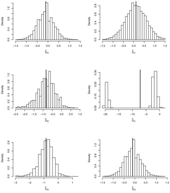
Shown in Figure 1 are distributions of parameter estimates obtained from 10,000 simulated datasets based on the QEM algorithm applied to the sparse problem. The bold vertical lines represent empirical means. It is clear that asymptotics does not kick in for the parameter related to sparse category that shows a distribution of point estimate β̂₃₁ markedly deviating from normal. When indexing regression coefficients we use first index to point to a specific contrast while the second index points at the value for the binary covariate. Its characteristic feature is a mixture component around −20. The other component of the mixed distribution scatters around the true value of the coefficient (−2.1). While the first component is negligible asymptotically, it represents the main source of instability in finite samples.

Figure 1.

Distribution of parameter estimates obtained from data simulated from a sparse model. First index of regression coefficient points at the category that is contrasted to the baseline category 1. Second index points at the value of the binary covariate.

Table 4 shows the empirical mean of β̂₃₁ deviating substantially from the true value used to simulate the data. The problem with category 3 is signalled by the large standard error of 8.13 for β̂₃₁ as compared to all other standard errors being an order of magnitude smaller.

The QEM algorithm, the Newton-Raphson algorithm and all simulation and data analysis of this paper were implemented in R. In this implementation we found the QEM to be somewhat slower than Newton Raphson in well-behaved problems as a consequence of nested iteration structure.

8 Analysis of Prostate Cancer Data

Prostate cancer screening in the US male population using the Prostate-Specific Antigen Test (PSA) induced a spike of the prostate cancer insidence and a change in the presentation of disease at diagnosis. Much of this dynamics is associated with so-called over-diagnosis Etzioni et al. (2002), a phenomenon that describes incidence of cancer that would not be detected without screening. Seeking to characterize the associated favorable shift in distribution of prostate cancer characteristics at diagnosis, we formulate a multinomial model of stage and grade of the disease regressed on covariates such as age, calendar time and race.

We use the QEM algorithm to analyze prostate cancer data from the Surveillance, Epidemiology and End Results (SEER) database (http://seer.cancer.gov/). A total of n = 251, 562 cancer cases from 1973 – 2001 are included in the analysis.

The multinomial outcomes are constructed from stage and histologic grade of the tumor. Staging is the assessment of the spread of prostate cancer. Due to difficulties distinguishing between regional and localized disease, SEER combines the stage into a binary variable with levels: (1) Localized (L), or Regional (R), and (2) Distant (D). The grade of tumor measured by the so-called Gleason score is the assessment of the degree of cell differentiation. Higher differentiated cells have lower grade and are less aggressive. SEER grade has 4 levels: (1) Well differentiated (W), (2) Moderately differentiated (M), (3) Poorly differentiated, and (4) Undifferentiated (U).

In this study, the multinomial outcome categories are formed by combining the levels of stage and grade. Four levels are formed based on the combined categories: (1) LRWM (2) LRPU (3) DWM and (4) DPU. In the analysis, LRWM is considered as the baseline category, which represents subjects diagnosed with a localized or regional stage tumor consisting of predominantly well or moderately differentiated cells.

Covariates in the study are Race [white (0), black (1)], Age (continuous), and Year modeling availability of PSA test [Before 1987 or No PSA (0), After 1987 or PSA (1)]. PSA test was approved by the FDA in 1986 and its use as a screening test for prostate cancer started after 1987.

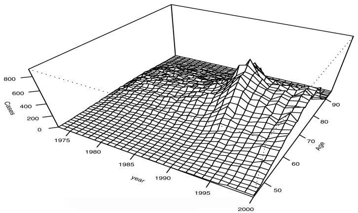
Shown in Figure 2 is a bivariate histogram of prostate cancer case count by age and calendar year. Increased incidence is evident around the introduction of PSA with the main impact occurring in the 60-80 age interval.

Figure 2.

Plot of Cases by Age and Year

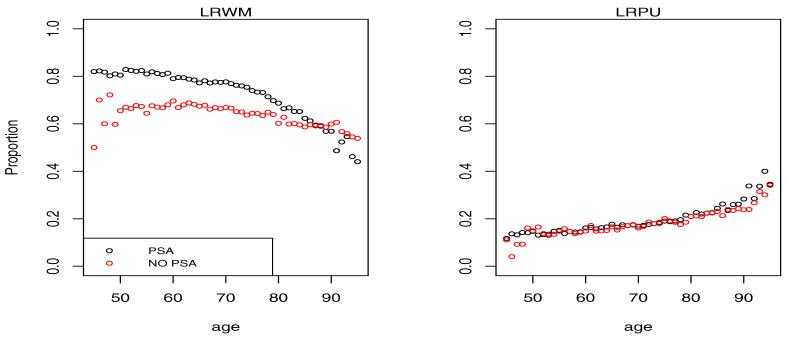
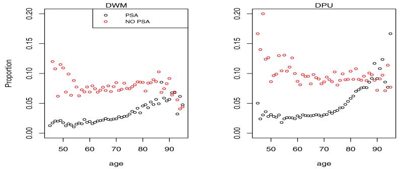
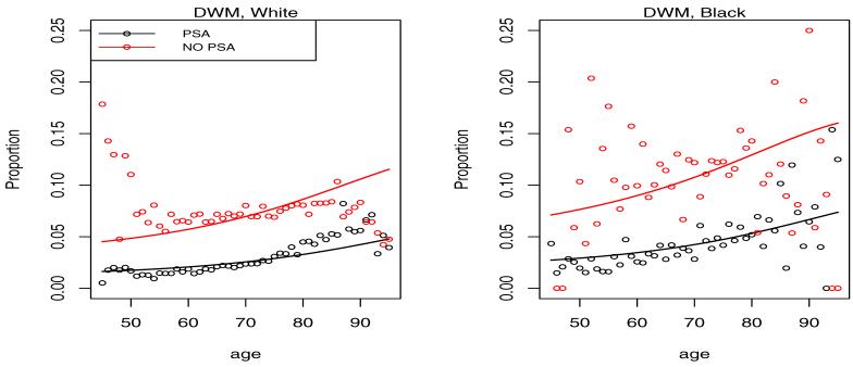
Shown in Figures 3 and 4 is the empirical multinomial distribution of the response representing fractions of cases in each of the 4 categories by calendar time (PSA vs. NO PSA) and age.

Figure 3.

Proportion of cases diagnosed in localized disease categories LRWM and LRPU by age and calendar time. The NO PSA plots refer to the calendar period before introduction of PSA in 1987, while the PSA plots refer to the period after 1987.

Figure 4.

Proportion of cases diagnosed in distant disease categories DWM and DPU by age and calendar time. The NO PSA plots refer to the calendar period before introduction of PSA in 1987, while the PSA plots refer to the period after 1987.

It is clear from the left plots in Figure 3 that the PSA has led to a shift of the presentation of the disease at diagnosis towards low grade localized disease. This is consistent with the intuition that overdiagnosed cancers when detected should present with the best prognosis. On the opposite end of the spectrum we see a reduction of the fraction of cases diagnosed in distant stage of the disease in Figure 4. With the probability mass shifting from worst to best categories with the introduction of PSA, the intermediate LRPU category has seen little change experiencing an in-flow associated with the reduced distant stage fraction and an outflow associated with increased LRWM fraction.

In order to confirm the above descriptive observations by statistical modeling a multinomial logit model was constructed as follows. With LRWM(1) as the reference category and c ∈ {LRPU(2), DWM(3), DPU(4)}, we have

$$\log \left\{\frac{\mathit{Pr}(Y=c)}{\mathit{Pr}(Y=1)}\right\}={\beta }_{c0}+{\beta }_{c1}\mathit{Year}+{\beta }_{c2}\mathit{Race}+{\beta }_{c3}\mathit{Age}+{\beta }_{c4}{\mathit{Age}}^2.$$

The quadratic age term was introduced to model the curvature of the effect of age seen on the descriptive plots.

Maximum likelihood estimates of the regression parameters and the associated standard errors are given in Table 5.

Table 5.

Model parameter estimates and standard errors (STE) resulting from an application of the QEM algorithm to fit a multinomial logit model to Prostate Cancer Data.

	contrasts
Variables	LRPU vs. LRWM	DWM vs LRWM	DPU vs LRWM
Intercept	−0.508 (0.228)	−2.579 (0.458)	0.848 (0.360)
Year	−0.113 (0.012)	−1.122 (0.020)	−1.013 (0.018)
Race	0.150 (0.017)	0.576 (0.028)	0.620 (0.025)
Age	−0.048 (0.007)	−0.020 (0.013)	−0.109 (0.010)
Age2	0.001 (0.0001)	0.0004 (0.0001)	0.001 (0.0001)

Parameter estimates indicate a favorable stage and grade shift with PSA reflected in negative Year coefficients modeling contrasts with the baseline best LRWM category. In addition, Blacks generally have worse disease than Whites (positive Race contrasts).

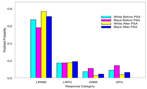
Figure 5 shows predicted probabilities by race and calendar period (PSA) at the median age (Age = 70yrs). It is evident that, irrespective of race, the predicted probability for subjects with localized/regional stage and well or moderately differentiated grade is higher with PSA. However, predicted probabilities for distant stage is smaller with PSA and Blacks have relatively worse tumor than Whites.

Figure 5.

Predicted Probabilities by Race and calendar period at median Age=70

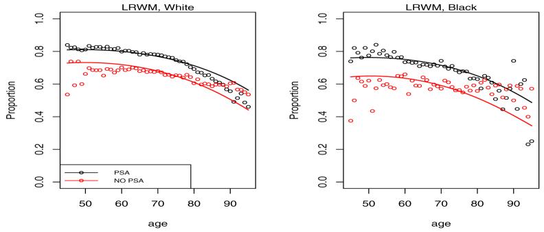
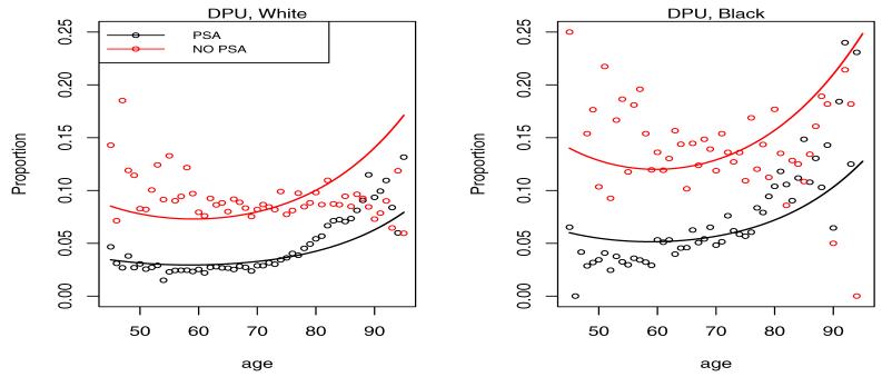
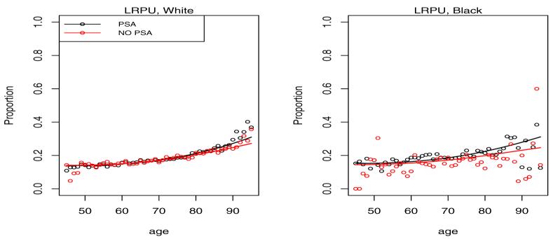
Figures 6-9 give plots of observed and predicted probabilities by age, period and race for each outcome category. The plots indicate a good agreement between observed and predicted probabilities except perhaps for men over 80 and under 50 because of their small fraction in the data.

Figure 6.

Predicted probability of LRWM diagnosis by age, race and period. PSA indicates a period after 1987, while NO PSA indicates a period before 1987.

Figure 9.

Predicted probability of DPU diagnosis by age, race and period. PSA indicates a period after 1987, while NO PSA indicates a period before 1987.

9 Discussion

EM algorithm can be viewed as a way to replace maximization of the original marginal likelihood by a different one corresponding to the complete-data model. The approach may offer advantages and increased stability if the problem at the complete-data level factors into a set of smaller problems. With this idea in mind, mixture models can be constructed artificially to replace a complex problem by a set of simpler and more convenient maximum likelihood problems at the cost of inducing a nested EM-like iteration structure.

For the multinomial model Poisson likelihood transformations have been attempted and justified by the method of Lagrange multipliers. However this solution is restricted to discrete covariates. The artificial mixture approach used in this paper also uses Poisson likelihood by manipulating the way normalizing restrictions on multinomial probabilities are enforced. However this is done by means of a mixture device rather than Lagrange penalties. This allowed us to lift the restrictions on covariates while at the same time reducing the dimension of maximization at the cost of introducing nested EM-like iterations.

Having informally constructed the desired algorithm we noticed that there is no probabilistic complete data model that corresponds to the Poisson likelihood being maximized at the M-step. In order to obtain justification of the algorithm we invoked a generalization of self consistency and expectation developped earlier. We used this opportunity to derive second order properties such as the information matrix in the generalized setting and applied it to the multinomial problem as an example.

Using simulations and real data analysis involving a large cancer registry dataset we found that the proposed QEM algorithm shows great stability and converged 100% of the time even when challenged by a sparse problem.

We have invoked the QEM construction using basis functions of the form u^ke^−su of an order up to k = 2 as was needed for the multinomial example. This corresponds to quasi-mixed models based on a QE operator that behave like ususal mixed models based on E up to the second moments of the mixing variable, i.e. conditional variances. It is possible to extend the construction for any order k, which remained beyond the scope of the present paper. This would be instrumental for repeated measurement models or models for clustered data such as shared frailty models in survival analysis. For example, extension to k = 3 would be needed for paired samples to model pairwise correlation. If an infinite number of subjects can potentially belong to one cluster (share same random intercept, for example), then the construction with k = 1,…,∞ would be needed. It can be shown that in this case QE=E, and the generality of the QE operator will be gone. In other words, QE behaving like E in terms of any conditional moment is an E. This follows from the fact that existence of all the derivatives of a Laplace transform makes it an analytic function and allows one to invert it and get the distribution of the random variable behind the transform, a constructive proof of its existence. However, the E-based formulation may still correspond to an artificial mixture model where the model at the complete-data level does not make sense in terms of probabilities, such as the multinomial model considered in this paper. In such cases, generalized self-consistency machinery would still be needed to justify the algorithms.

The fact that the likelihood transformation is accomplished by means of expectation (a key tool of Bayesian inference) rather than maximization would make this methodology potentially useful in the Bayesian context.

The example of this paper indicates that an EM-like device can be used as a method of obtaining maximum likelihood estimates under restrictions as an attractive alternative to Lagrange multipliers when dimension reduction is preferrable.

Figure 7.

Predicted probability of LRPU diagnosis by age, race and period. PSA indicates a period after 1987, while NO PSA indicates a period before 1987.

Figure 8.

Predicted probability of DWM diagnosis by age, race and period. PSA indicates a period after 1987, while NO PSA indicates a period before 1987.

1 Appendix. The generalized missing information principle

Let

$$L_0(\beta \mid U),{\ell }_0(\beta \mid U)=\log L_0(\beta \mid U)$$

be a complete-data likelihood where first argument is a parameter vector, and second argument is a surrogate of random missing data U, an argument to be used by the QE-transform. Suppose, the likelihood for a model of interest is defined as a transform

$$L\left(\beta \right)=\mathrm{QE}\left\{L_0(\beta \mid U)\right\},\ell \left(\beta \right)=\log L\left(\beta \right)$$

where QE is a functional operator that acts on L₀ considered as an admissible function of U belonging to a functional space where QE is defined. Then the score function is represented as a conditional QE given complete-data likelihood L₀ as

$$\frac{\partial \ell \left(\beta \right)}{\beta }=\frac{\frac{\partial }{\partial \beta }\mathrm{QE}\left\{L_0(\beta \mid U)\right\}}{\mathrm{QE}\left\{L_0(\beta \mid U)\right\}}=\frac{\mathrm{QE}\left\{\frac{\partial {\ell }_0\left(\beta \right)}{\partial \beta }{L}_0(\beta \mid U)\right\}}{\mathrm{QE}\left\{L_0(\beta \mid U)\right\}}=\mathrm{QE}\left\{\phantom{\mid }\frac{\partial {\ell }_0\left(\beta \right)}{\partial \beta }\mid L_0(\beta \mid U)\right\},$$

using the definition of conditional QE (17), and interchangeability of QE and differentiation (16). The latter expression is a foundation for the EM and QEM iterative procedure (19). Taking a second derivative with respect to vector of parameters β, we have along similar lines

$$\begin{array}{c}\hfill I=-\frac{\partial }{\partial \beta }\mathrm{QE}\left\{\phantom{\mid }\frac{\partial {\ell }_0(\beta \mid U)}{\partial {\beta }^{\mathrm{T}}}\mid L_0(\beta \mid U)\right\}=-\frac{\mathrm{QE}\left\{\frac{{\partial }^2{\ell }_0(\beta \mid U)}{\partial \beta \partial {\beta }^{\mathrm{T}}}{L}_0(\beta \mid U)\right\}}{\mathrm{QE}\left\{L_0(\beta \mid U)\right\}}-\hfill \\ \hfill \frac{\mathrm{QE}\left\{\frac{\partial {\ell }_0(\beta \mid U)}{\partial \beta }\frac{\partial {\ell }_0(\beta \mid U)}{\partial {\beta }^{\mathrm{T}}}{L}_0(\beta \mid U)\right\}}{\mathrm{QE}\left\{L_0(\beta \mid U)\right\}}+\frac{\partial \ell \left(\beta \right)}{\partial \beta }\frac{\partial \ell \left(\beta \right)}{\partial {\beta }^{\mathrm{T}}}=\hfill \\ \hfill -\mathrm{QE}\left\{\phantom{\mid }\frac{{\partial }^2{\ell }_0(\beta \mid U)}{\partial \beta \partial {\beta }^{\mathrm{T}}}\mid L_0(\beta \mid U)\right\}-\mathrm{QE}\left\{\phantom{\mid }\frac{\partial {\ell }_0(\beta \mid U)}{\partial \beta }\frac{\partial {\ell }_0(\beta \mid U)}{\partial {\beta }^{\mathrm{T}}}\mid L_0(\beta \mid U)\right\}+\frac{\partial \ell \left(\beta \right)}{\partial \beta }\frac{\partial \ell \left(\beta \right)}{\partial {\beta }^{\mathrm{T}}}.\hfill \end{array}$$

We now get the partitioning of observed information (30) on noting that in the latter expression, at the point of MLE,

$$\frac{\partial \ell \left(\beta \right)}{\partial \beta }=0.$$

End of proof.

2 Appendix. Quasi-Variance

In this Appendix we will prove the relationship between V(x) as given in terms of Θ by (34) and also in terms of the derivative of Θ(x|0) as given by (37). Consider an analog of Laplace transform defined using the QE-operator

$$\mathcal{L}\left(s\right)=\gamma \left(e^{-s}\right)=\mathrm{QE}\left\{x^U\right\},x=e^{-s}.$$

Then by interchangeability of QE and differentiation

$$\begin{array}{cc}\hfill \mathrm{QE}\left\{x^U\right\}& =\gamma \left(x\right)=\mathcal{L}\left(s\right)\hfill \\ \hfill \mathrm{QE}\left\{U{x}^U\right\}& =x\gamma \left(x\right)=-{\mathcal{L}}^{\prime }\left(s\right)\hfill \\ \hfill \mathrm{QE}\left\{U^2{x}^U\right\}& =x{\gamma }^{\prime }\left(x\right)+x^2{\gamma }^{″}\left(x\right)={\mathcal{L}}^{″}\left(s\right)\hfill \end{array}$$ (42)

Using the above relationships, we have

$$\begin{array}{cc}\hfill \mathrm{QE}\{U\mid x^U\}=\frac{\mathrm{QE}\left\{U{x}^U\right\}}{\mathrm{QE}\left\{x^U\right\}}& =-\frac{{\mathcal{L}}^{\prime }\left(s\right)}{{\mathcal{L}}^{\prime }\left(s\right)}\hfill \\ \hfill \mathrm{QE}\{U^2\mid x^U\}=\frac{\mathrm{QE}\left\{U^2{x}^U\right\}}{\mathrm{QE}\left\{x^U\right\}}& =\frac{{\mathcal{L}}^{″}\left(s\right)}{\mathcal{L}\left(s\right)},\hfill \end{array}$$ (43)

which in turn yields

$$\begin{array}{cc}\hfill \Theta (x\mid 0)=\frac{\mathrm{QE}\left\{U{x}^U\right\}}{\mathrm{QE}\left\{x^U\right\}}& =-\frac{{\mathcal{L}}^{\prime }\left(s\right)}{{\mathcal{L}}^{\prime }\left(s\right)}\hfill \\ \hfill \Theta (x\mid 1)=\frac{\mathrm{QE}\left\{U^2{x}^U\right\}}{\mathrm{QE}\left\{U{x}^U\right\}}& =\frac{{\mathcal{L}}^{″}\left(s\right)}{{\mathcal{L}}^{\prime }\left(s\right)}.\hfill \end{array}$$ (44)

Now, using (43) and (44)

$$\begin{array}{c}\hfill \mathrm{QVar}\{U\mid x^U\}=\mathrm{QE}(U^2\mid x^U)-{\mathrm{QE}}^2(U\mid x^U)=\frac{{\mathcal{L}}^{″}\left(s\right)}{\mathcal{L}\left(s\right)}-{\left[\frac{{\mathcal{L}}^{\prime }\left(s\right)}{\mathcal{L}\left(s\right)}\right]}^2=\hfill \\ \hfill -\frac{{\mathcal{L}}^{\prime }\left(s\right)}{\mathcal{L}\left(s\right)}\left[\frac{{\mathcal{L}}^{″}\left(s\right)}{{\mathcal{L}}^{\prime }\left(s\right)}-\left(-\frac{{\mathcal{L}}^{\prime }\left(s\right)}{\mathcal{L}\left(s\right)}\right)\right]=\Theta (x\mid 0)[\Theta (x\mid 1)-\Theta (x\mid 0)]=\mathcal{V}\left(x\right).\hfill \end{array}$$

Thus the (34) connection is now established. Now, in terms of the derivative of Θ(x|0), x = e^−s, we have

$$\begin{array}{c}\hfill \frac{\partial }{{\partial }_s}\Theta (e^{-s}\mid 0)=\Theta (x\mid 0)\frac{\partial }{{\partial }_s}\log \Theta (x\left(s\right)\mid 0)=\hfill \\ \hfill \Theta (x\mid 0)\{{\left(\log [-{\mathcal{L}}^{\prime }\left(s\right)]\right)}^{\prime }-{\left(\log [-\mathcal{L}\left(s\right)]\right)}^{\prime }\}=\Theta (x\mid 0)\left[\frac{{\mathcal{L}}^{″}\left(s\right)}{{\mathcal{L}}^{\prime }\left(s\right)}-\frac{{\mathcal{L}}^{\prime }\left(s\right)}{\mathcal{L}\left(s\right)}\right]=\hfill \\ \hfill -\Theta (x\mid 0)[\Theta (x\mid 1)-\Theta (x\mid 0)]=-\mathcal{V}\left(x\right)\hfill \end{array}$$

as in (37). End of proof.

3 Appendix. Missing information for a log-linear “complete-data” likelihood

In this Appendix we show that a form of the “complete-data” likelihood kernel (31) that is log-linear in “missing data” implies (32) and (33). We have

$${\ell }_{\mathrm{CD}}=-A\left(\beta \right)u+B\left(\beta \right).$$

Therefore,

$${\mathcal{I}}_{\mathrm{CD}}=\frac{{\partial }^{2}A\left(\beta \right)}{\partial \beta \partial {\beta }^{\mathrm{T}}}u-\frac{{\partial }^{2}B\left(\beta \right)}{\partial \beta \partial {\beta }^{\mathrm{T}}}.$$

Applying QE {·|L_CD} to the above expression and noting that

$$\Theta (e^A\mid 0)=\mathrm{QE}\{U\mid e^{-\mathit{AU}+B}\}$$

for any A and B that do not depend on u, we get (32). Now,

$$\begin{array}{c}\hfill {\mathcal{I}}_{\mathrm{MD}}=\frac{\partial {\ell }_{\mathrm{CD}}(U,\beta )}{\partial \beta }\frac{\partial {\ell }_{\mathrm{CD}}(U,\beta )}{\partial {\beta }^{\mathrm{T}}}=\frac{\partial A\left(\beta \right)}{\partial \beta }\frac{\partial A\left(\beta \right)}{\partial {\beta }^{\mathrm{T}}}{U}^2-\hfill \\ \hfill \left[\frac{\partial A\left(\beta \right)}{\partial \beta }\frac{\partial B\left(\beta \right)}{\partial {\beta }^{\mathrm{T}}}+\frac{\partial B\left(\beta \right)}{\partial \beta }\frac{\partial A\left(\beta \right)}{\partial {\beta }^{\mathrm{T}}}\right]U+\frac{\partial B\left(\beta \right)}{\partial \beta }\frac{\partial B\left(\beta \right)}{\partial {\beta }^{\mathrm{T}}}\hfill \end{array}$$

Applying QE {·|L_CD} to the above expression and noting that

$$\mathrm{QVar}\{U\mid L_{\mathrm{CD}}\left(U\right)\}=\mathrm{QE}\{U^2\mid L_{\mathrm{CD}}\left(U\right)\}-{\mathrm{QE}}^2\{U\mid L_{\mathrm{CD}}\left(U\right)\},$$

and that

$$\begin{array}{cc}\hfill \mathrm{QE}& \left\{\frac{\partial {\ell }_{\mathrm{CD}}(U,\beta )}{\partial \beta }\right\}\mathrm{QE}\left\{\frac{\partial {\ell }_{\mathrm{CD}}(U,\beta )}{\partial {\beta }^{\mathrm{T}}}\right\}=\frac{\partial A\left(\beta \right)}{\partial \beta }\frac{\partial A\left(\beta \right)}{\partial {\beta }^{\mathrm{T}}}{\mathrm{QE}}^2\{U\mid L_{\mathrm{CD}}\left(U\right)\}-\hfill \\ \hfill & \left[\frac{\partial A\left(\beta \right)}{\partial \beta }\frac{\partial B\left(\beta \right)}{\partial {\beta }^{\mathrm{T}}}+\frac{\partial B\left(\beta \right)}{\partial \beta }\frac{\partial A\left(\beta \right)}{\partial {\beta }^{\mathrm{T}}}\right]\mathrm{QE}\{U\mid L_{\mathrm{CD}}\left(U\right)\}+\frac{\partial B\left(\beta \right)}{\partial \beta }\frac{\partial B\left(\beta \right)}{\partial {\beta }^{\mathrm{T}}}\hfill \end{array}$$

we have

$${\mathcal{I}}_{\mathrm{MD}}=\mathrm{QE}\left\{\frac{\partial {\ell }_{\mathrm{CD}}(U,\beta )}{\partial \beta }\right\}\mathrm{QE}\left\{\frac{\partial {\ell }_{\mathrm{CD}}(U,\beta )}{\partial {\beta }^{\mathrm{T}}}\right\}+\frac{\partial A\left(\beta \right)}{\partial \beta }\frac{\partial A\left(\beta \right)}{\partial {\beta }^{\mathrm{T}}}\mathrm{QVar}\{U\mid L_{\mathrm{CD}}\left(U\right)\}$$

At the point of MLE the first term in the last expression is zero while the last term is equal to the right part of (33). End of proof.

References

- Baker S. Thes Multinomial-Poisson transformation. The Statistician. 1994;43:495–504. [Google Scholar]
- Conaway M. The analysis of repeated categorical measurements subject to nonignorable nonresponse. Journal of the american Statistical Association. 1992;87:817–824. [Google Scholar]
- Cormack RM. Discussion on a simple EM algorithm for capture-recapture data with categorical covariates (by S. G. Baker) Biometrics. 1990;46:1193–1200. [PubMed] [Google Scholar]
- Etzioni R, Penson D, Legler J, Tommaso D. d., Boer R, Gann P, Feuer E. Prostate-specific antigen screening: Lessons from U.S. prostate cancer incidence trends. Journal of the National Cancer Institute. 2002;13:981–990. doi: 10.1093/jnci/94.13.981. [DOI] [PubMed] [Google Scholar]
- Ghosh M, Zhang L, Mukherjee B. Equivalence of posteriors in the Bayesian analysis of the Multinomial-Poisson transformation. Metron. 2006:19–28. [Google Scholar]
- Lang J. On the comparison of multinomial and Poisson log-linear models. Journal of the Royal Statistical Society, Series B: Statistical Methodology. 1996;58:253–266. [Google Scholar]
- Louis TA. Finding the observed information matrix when using the EM algorithm. Journal of the Royal Statistical Society, Series B: Statistical Methodology. 1982;4(2):226–233. [Google Scholar]
- Oakes D. Direct calculation of the information matrix via the EM algorithm. Journal of the Royal Statistical Society, Series B: Statistical Methodology. 1999;67(3):479–482. [Google Scholar]
- Palmgren J. The Fisher information matrix for log linear models arguing conditionally on observed explanatory variables. Biometrika. 1981;68:563–566. [Google Scholar]
- Tiur T. A connection between Rasch's item analysis model and a multiplicative poisson model. Scandinavian Journal of Statistics. 1982;9:23–30. [Google Scholar]
- Tsodikov A. Semiparametric models: A generalized self-consistency approach. Journal of the Royal Statistical Society, Series B: Statistical Methodology. 2003;65(3):759–774. doi: 10.1111/1467-9868.00414. [DOI] [PMC free article] [PubMed] [Google Scholar]
- Whitehead J. Fitting Cox's regression model to survival data using GLIM. Applied Statistics. 1980;29:268–275. [Google Scholar]