Unmasking Imaging Forces on Soft Biological Samples in Liquids When Using Dynamic Atomic Force Microscopy: A Case Study on Viral Capsids

Abstract

Dynamic atomic force microscopy is widely used for the imaging of soft biological materials in liquid environments; yet very little is known about the peak forces exerted by the oscillating probe tapping on the sample in liquid environments. In this article, we combine theory and experiments in liquid on virus capsids to propose scaling laws for peak interaction forces exerted on soft samples in liquid environments. We demonstrate how these laws can be used to choose probes and operating conditions to minimize imaging forces and thereby robustly image fragile biological samples.

INTRODUCTION

A major goal in the imaging of biological samples is to reconstruct with nanometer resolution the quasinative state of biological membranes, proteins, DNA, and macromolecular complexes in their physiological buffer solutions. Dynamic atomic force microscopy (dAFM) is arguably the leading tool to address this goal. In dAFM, an oscillating cantilever with a sharp nanoscale tip interacts intermittently with the sample, introducing short- and long-range tip-sample interaction forces while it is scanning over the sample surface. Our focus in this article is on the more commonly used amplitude modulated mode, which is also known as the tapping mode (TM). Historically, average forces have been considered the most relevant parameter to obtain reproducible AFM images of soft samples in liquids (1). Average forces are relatively easy to measure with optical beam deflection methods; however, recent results (2) indicate that the peak forces can play a far more significant role, especially when scanning fragile biological samples in dynamic modes. Peak forces of the order of even a few nanonewtons can irreversibly deform the macromolecule being imaged. Thus the peak interaction forces are, in fact, the imaging forces exerted on the sample during the scan. The peak forces also provide direct insight into the physics of nanoscale adhesion, elasticity, viscoelasticity, or specific molecular interactions (3–7) on the biological samples.

Unfortunately, measuring peak forces in liquids is not as simple as measuring average forces. This is probably one of the reasons, despite the great importance of imaging forces, that very little is quantitatively understood about the influence of probe and sample properties and other experimental conditions on the peak interaction forces exerted on soft samples in liquid environments. For example, let us consider experiments performed on the Bacillus subtilis phage Φ29 in physiological solution (specifically in TMS buffer (50 mM Tris, 10 mM MgCl₂, 100 mM NaCl) with pH 7.8) using two different cantilevers that we name conventional lever (CL) and small lever (SL) (Table 1 summarizes the relevant parameters of both cantilevers as specified by the manufacturer, and Table 2 gives the typical values measured or calibrated in the laboratory).

TABLE 1.

Typical properties of SL and CL specified by the manufacturer

	(SL) BioLever*	(CL) OMCL-RC800PSA†
L(μm) × b(μm) × h(μm)	60 × 30 × 0.18	200 × 20 × 0.8
Tip height (μm)	7	2.9
Tip radius (nm)	30	20
Nominal stiffness (N/m)	0.03	0.05
Resonance frequency in air (kHz)	37	18

^*Available at http://probe.olympus-global.com, BL-RC150VB.

^†Available at http://probe.olympus-global.com, OMCL-RC800PSA.

TABLE 2.

Typical measured properties (in laboratory) of SL and CL corresponding to Fig. 5

	(SL) BioLever	(CL) OMCL-RC800PSA
Resonance frequency in air (kHz)	43.6	20.1
Q-factor in air	41	53
Resonance frequency in liquid: far from surface (kHz)	9.3	6.0
Resonance frequency in liquid: close to surface (kHz)	8.3	5.4
Q-factor in liquid: far from surface	1.84	1.85
Q-factor in liquid: close to surface	1.02	0.47
Cantilever stiffness* (N/m)	0.063	0.072
Effective mass in liquid: close to surface (kg)	1.9 × 10−11	5.2 × 10−11
Effective mass in liquid: close to surface (kg)	2.4 × 10−11	6.4 × 10−11

^*Calibrated by Sader's method (9).

Images are taken using TM-AFM by acoustically exciting the cantilevers with a dither piezo at a frequency equaling that of the thermal resonance. Fig. 1 shows micrographs of the two cantilevers (note the tip of the SL is significantly larger than that of the CL) and the phage Φ29 imaged with both types of cantilevers under the best possible operating conditions for each of them (free amplitude vibration used is 20 nm, and the amplitude setpoint ratio is ∼82% and 65% for CL and SL, respectively). Using the SL, images as in Fig. 1 c are obtained routinely and the structure of the virus is intact, showing the nominal height of 50 nm (8); however, when the CL is used, images such as those in Fig. 1 d are always obtained showing a damaged virus. We obtained similar results with the parvovirus minute virus of mice (MVM). These results clearly suggest that the CL typically applies far greater imaging forces on the viral capsids compared to the SL leading to their irreversible rupture. Additional experiments performed on microtubules in buffer solutions confirm the larger imaging forces applied to soft biological samples by the CL compared to the SL.

FIGURE 1.

Scanning electron micrographs of the (a) SL and (b) CL (see Table 1 for properties) used for this study and phage Φ29 capsids imaged with the SL and the CL using acoustic dAFM under nominally similar operating conditions. Note the scale bar in (a) and (b) are the same, indicating the tip length of the SL is much larger than that of the CL. (c) A TM image of the viral capsid taken with the SL with the inset profile showing the correct height of the capsid. (d) A TM image of the same kind of capsid scanned with the CL with the inset profile showing a collapsed virus capsid. The virus is repeatably damaged under similar imaging conditions as the SL. Similar results are obtained with the MVM virus.

A natural question that arises is: what factors cause such a significant difference in the imaging forces exerted by the two cantilevers? The nominal stiffness of the SL is only 40% less than that of the CL, and their resonance Q-factors far from the surface are comparable (Table 1 and 2). The number of possible influential factors is large; the cantilever stiffness, Q-factor, resonance frequency, effective mass ( where k_eff = 1.0302k_c (k_c is the cantilever stiffness calibrated by the Sader's method (9)) is the effective cantilever stiffness for the first flexural mode (10), ω₀ is the angular resonance frequency of the first eigenmode), and the dimensions of the cantilever may all be important. Unfortunately, very few theoretical tools are available to the experimentalist to answer this critical question.

In this article, we systematically identify by means of nonlinear dynamics theory and experiments the power law dependence of the imaging forces in liquids on the important factors and provide a rational explanation to the results in Fig. 1. We perform detailed experiments using the recently developed scanning probe acceleration microscopy (SPAM) (2) to measure imaging forces on the Bacillus subtilis phage Φ29 and the parvovirus MVM since their mechanical response is known (11,12). The analytical expressions for the peak forces presented in the form of power laws provide a reasonable estimate of the experimental imaging forces on these soft samples and provide clear insight into the most important criteria that lead to reduced imaging forces on soft biological samples in liquid environments. Moreover, our experimental results confirm prior works on the mechanical forces required for capsid collapse and may provide insights into the viscoelastic properties of viral shells.

THEORY

In developing a simple mathematical model for TM-AFM that can be used to predict the peak interaction forces, two key simplifying assumptions are made:

1. When the cantilever is driven in a specific eigenmode in liquids far from the sample, it can be appropriately modeled as a driven, damped harmonic oscillator with effective modal properties. In what follows, we assume that this point mass model continues to hold when the oscillating cantilever is brought closer to the sample. Recent work (13) has shown that the second mode also needs to be included to accurately predict tip motion when the cantilever taps on a sample in liquid environments. However, in the pursuit of explicit analytical expressions for imaging forces, we assume that the contributions to imaging forces from the second mode are negligible. Indeed the work of Basak (14) suggests that neglect of the second mode can lead to a 10%–15% error in the prediction of peak forces.

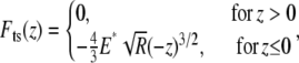
2. For dAFM applications in liquids, there are two common modes of exciting the cantilever, the so-called magnetic mode (15) and the acoustic mode (16). Recent work (17,18) has demonstrated that there are important differences between these two modes, especially while using soft cantilevers in liquid environments. Specifically, the observable quantity in acoustic mode excitation is the difference between the tip motion and the dither piezo motion, whereas in the magnetic mode the absolute tip motion is observed (Fig. 2). Additionally in acoustic mode the cantilever is, for the most part, excited by the unsteady fluid forces arising from the vibration of the dither piezo in the liquid cell. However, as we will see in the acoustic mode experiments described later, the dither piezo motion is much smaller than the tip motion for large amplitude setpoint; so the difference between actual tip motion and the observed motion can be assumed to be negligible for our experiments.

FIGURE 2.

Schematic of a cantilever tapping a virus capsid by (a) acoustic mode and (b) magnetic mode. In magnetic mode, the measured tip motion is the absolute tip motion, whereas in the acoustic mode the measured motion (transverse cantilever deflection) is the tip motion relative to the chip motion. (c) A schematic of the model employed in this work.

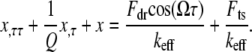
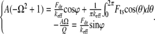
Thus, the simple, single degree-of-freedom model that describes the tip motion in TM in liquids becomes (2,13)

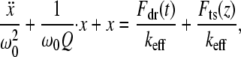(1)

where is the effective cantilever stiffness for the first flexural mode (10), is the drive force from fluid-borne excitation, is the tip-sample interaction force, and is absolute tip motion. If is the instantaneous gap between the tip and the sample, then 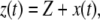where is the average gap between the tip and the sample (Fig. 2 c). is the quality factor and is the angular resonance frequency of the eigenmode in liquid. Note that and are strongly influenced by the hydrodynamics, which in turn are dependent on the proximity of the cantilever to the sample. In principle and can be computed a priori using hydrodynamic functions close to the sample (14,19), or they can be experimentally determined when the cantilever is close enough to the sample to begin imaging using the thermal noise method. The latter strategy is adopted in this work.

To model the tip-sample interaction force in liquids, we note that in the vicinity of the sample the tip experiences mainly the van der Waals forces and the electric double layer forces. This interaction is usually described by the Derjaguin-Landau-Verwey-Overbeek theory (20). However, at high salt concentration, such as in the imaging buffer used in our experiments, the Debye length is short enough (<0.8 nm for both our experiments) that the electric double layer forces can be neglected. In the experiments to be described later, sharp AFM tips with a radius of ∼10 nm are tapping on a hard substrate surface (glass or mica) or on soft (MVM is the hardest virus we have ever found, but it is soft compared with glass or mica) virus capsids in buffer solutions. In such cases, the van der Waals force and any other force have little effect compared to the large repulsive elastic contact force when the tip is in contact with the sample. So we consider only the elastic contact force in our tip-sample interaction model.

When the tip is tapping the hard glass or mica surface, we model the tip-sample interaction force using the Hertz contact model (21):

(2)

where is the tip radius, is the instantaneous tip-sample separation, and is the effective elastic modulus of tip and sample and is given by

(3)

where and are the Poisson's ratio and Young's modulus of the tip and sample, respectively. When the tip is tapping on the virus capsids, linear elastic response for the indentation is expected from thin shell mechanics (22) and was observed in experiments (11). Thus, the tip-sample interactions for small capsid indentations can be modeled as a linear spring:

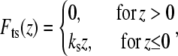(4)

where is the effective spring constant of the samples measured from experimental force-distance curves in liquids.

To derive closed form approximate analytical solutions to peak forces using Eqs. 1–4, we employ the one-term Harmonic balance method commonly used in the nonlinear dynamics community (23). Introducing 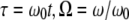into Eq. 1, we get

(5)

In the one-term harmonic balance method, it is assumed that the tip oscillates periodically This is substituted into the expression for interaction force (Eq. 2 or 4), and the first Fourier component of can be calculated as follows:

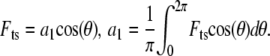(6)

Substituting Eq. 6 into Eq. 5, we get the following integral relations for TMAFM:

(7)

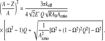
By assuming that the indentation is small, and for we are able to analytically approximate the integral term above (see Appendix 1 for details); and eliminating the phase from the above equations, we find that the peak repulsive interaction force for the Hertz contact model 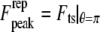is given by

(8)

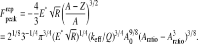
where is the initial (free) amplitude and is the amplitude setpoint ratio. Similarly, for the linear contact indentation model for thin shell virus capsids, the formula for peak repulsive force is (See Appendix 1 for details)

(9)

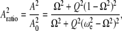
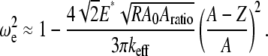
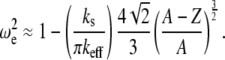
The peak force expressions Eq. 8 (for Hertz contact model) and Eq. 9 (for linear contact indentation) are exactly the same as the peak force formulas for the high-Q factor AFM situations given in Hu and Raman (24) and Hu (25), which are derived by the averaging method (26). Because the averaging method cannot be extended to low-Q situations, we adopted the harmonic balance method, which is valid for very low Q-factor situations and also, in fact, for overdamped oscillators. These compact analytical expressions (Eqs. 8 and 9), of course, come with certain assumptions which must be met for them to provide valid predictions. First, these formulas apply only to small indentations of the sample. Second, they are derived for the case when the drive frequency equals the frequency of the thermal peak. Third, here we use only the first harmonic term, and as we discussed earlier the higher harmonics will contribute substantially to the peak interaction force at lower amplitude setpoint ratios () in liquid environments. Thus these formulas give us a good sense of the scaling laws for peak interaction forces exerted on soft samples in liquids for small indentations (or equivalently, at high amplitude setpoint ratios).

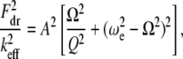
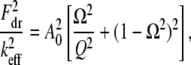
From Eqs. 8 and 9, we can see that for the same sample and similar operating conditions (equal and ), the imaging forces scale by or for viral shells and flat elastic substrates, respectively. In what follows, we compare the predictions of the peak force formulas and mathematical simulations of Eq. 1 with experimental results.

EXPERIMENTAL PROCEDURES, MATERIALS, AND METHODS

AFM of viral samples

Stocks of empty capsid of Φ29 and empty capsid of MVM were used in TMS buffer (50 mM Tris, 10 mM MgCl₂, 100 mM NaCl, pH 7.8) and PBS buffer (137 mM NaCl, 2.7 mM KCl, 1.5 mM NaH₂PO₄, 8.1 mM KH₂PO₄, pH 7.2), respectively. For both cases, a single drop of 20 μl stock solution capsid was deposited on a silanized glass surface (11), which was left for 30 min on the surface and washed with buffer. The tip was prewetted with 20 μl of buffer.

The AFM (Nanotec Electrónica S.L., Madrid, Spain) was operated in acoustic dynamic mode (TM-AFM) in liquid, and the images were processed using the WSxM software (Nanotec Electrónica S.L., Madrid, Spain) (27). Once a virus particle was successfully imaged, the oscillating probe was made to approach the center of the virus particle while the cantilever's time deflection history was recorded. The time series data were acquired repeatedly using the SL for different and values on both the MVM and Φ29 procapsids. To ensure good signal reconstruction, the deflection data were captured at a sampling frequency of 5–20 MHz. Fig. 3 shows typical oscillation waveforms upon approach to the sample. Tip-sample intermittent contacts can be seen as local harmonic distortions in the waveform. Even when the cantilever comes in full, continuous contact with the sample, a “residual” oscillation waveform is still recorded. This is because the dither piezo continues to vibrate even when the cantilever is in full contact. The amplitude of the residual oscillation clearly equals the dither piezo amplitude. As can be seen from Fig. 3, the dither piezo motion is much smaller compared to the free amplitude measured; so certainly for larger amplitude setpoint ratios, it is reasonable to assume that the observed tip motion is sufficiently close to the actual tip motion. This observation justifies the second assumption in the theoretical model.

FIGURE 3.

Waveforms acquired from experimental approach curves using the SL probe made on top of (a) Φ29 (b) MVM virus capsids. The characteristic distortion of the deflection signal caused by intermittent contact with the sample can be clearly seen from the inset figure. Moreover, the dither piezo motion A_residual is much smaller compared to the free amplitude of the tip, at least for large amplitude setpoints that are typically used for imaging.

Acceleration spectroscopy to extract peak interaction forces

To extract the tip-sample interaction forces from the experimental approach curves (Fig. 3), we used the SPAM (2) method. Rearranging Eq. 1, we have

(10)

Since the contribution to the acceleration of the pulse-like tip-sample interaction force can be easily distinguished from other slowly varying and small magnitude forces, this gives us a simple way to reconstruct the imaging force. For this method to be applied to real noisy experimental data (Fig. 4 a, points), the measured deflection signals need “comb-filtering” (2), in which only the intensities at integer harmonic frequencies are retained in the Fourier spectrum to reconstruct the deflection signal (Fig. 4 a, solid curve). Similar curves are acquired with different but nominally similar cantilevers with different initial amplitudes, and the results are quite reproducible.

FIGURE 4.

SPAM of the SL probe on MVM. (a) Original (point) and comb-filtered (solid) deflection signals on MVM and the acceleration of the comb-filtered deflection signal (dash). The pulse in the acceleration signal corresponds to the tip-sample interaction. (b) Peak forces extracted from the experimental approach curve.

By multiplying the acceleration of the reconstructed deflection signal (Fig. 4 a, dashed curve) with the effective mass, we are able to reconstruct the peak forces from each approach curve and extract the peak force from the experimental data as shown in Fig. 4 b (details provided in Appendix 2). The 10-point moving averages of the experimental peak force data are also plotted in Fig. 4 b.

The method described above uses the SPAM method to extract peak forces while the cantilever continuously approaches the sample, which means that the deflection signal is nonstationary. We systematically studied this effect by collecting and analyzing data at different, slower approach speeds and even with the cantilever oscillating at fixed distances from the sample and found the errors in peak force prediction to be minimal, at least for the approach speeds we used in our experiments.

RESULTS

Before proceeding to compare peak interaction forces upon approach to the sample, it is important to understand how the proximity of the surface affects the cantilever motion. In Fig. 5, we plot the experimental thermal vibration spectra (Brownian motion excited response) of both the levers in a) air, b) buffer solution far from the sample, and c) buffer solution within imaging distance from the sample. We notice the Q-factors of the SL and CL decrease significantly due to a hydrodynamic squeeze film effect between the oscillating lever and the sample surface. More importantly, although the two levers possess comparable Q-factors far from the sample, the Q-factor near the sample of the SL (Q ∼ 1) is two times larger than that of the CL (Q ∼ 0.5). In fact, the CL becomes overdamped when within imaging distance from the sample, implying that no resonance peak can be found in its thermal vibration spectrum. This has a major influence on the imaging force exerted by the CL, as we will see in the following discussion.

FIGURE 5.

Thermal spectrum (Brownian motion excited) of SL and CL in air and liquid far and close to the surface. The values of the Q factor are indicated in the graphs. (a) Thermal spectrum for SL is represented showing the decrease of the Q factor in liquid when it is close to the sample. (b) Thermal spectrum for CL is represented showing the overdamped behavior when it is close to the surface.

Approach curves on both virus capsids with different initial amplitudes (12 nm ∼ 49 nm) have been recorded. Because small initial amplitudes lead to a low signal/noise ratio, we present here the extracted peak forces using approach curves with a sufficiently large initial amplitude. Fig. 6 shows typical experimental peak force extracted by the SPAM method (dashed curve) compared with the numerical simulation results (point/solid curve) using Eq. 5 and the analytical prediction (dotted curve) using Eq. 9 on both Φ29 and MVM capsids. The simulations are performed with SIMULINK and MATLAB (The MathWorks, Natick, MA), and the analytical prediction are presented using Eq. 9, both using the nominal parameter values listed in Table 3 that have been extracted from experimental data.

FIGURE 6.

Peak interaction forces on (a) Φ29 and (b) MVM with inset of AFM images. The dashed curves are experimental data extracted by the acceleration method (smoothed using 10-point moving average), the point/solid curves are predictions from mathematical simulations using Eqs. 1 and 4 along with the error bars (standard deviation), and the dotted curves are the analytical prediction using Eq. 9 using parameters in Table 3.

TABLE 3.

Experimental conditions corresponding to Figs. 4 and 6

	Φ29	MVM
Cantilever stiffness* (N/m)	0.050	0.062
Q-factor in liquid: close to surface	1.0	1.0
Resonance frequency in liquid: close to surface (Hz)	8346	8381
DAQ Sampling rate	2 × 107	5 × 106
Free peak-peak amplitude (nm)	46	49
Sample stiffness (N/m)	0.3	0.6

^*Calibrated by Sader's method (9).

The analytical peak force predictions are generally found to come within 20% of the numerically simulated data for amplitude setpoint ratios >80%. As the amplitude setpoint ratio decreases, the small indentation assumption is no longer valid and the analytical formula diverges from the numerically simulated data. However, it still gives a reasonable prediction at moderate indentation. For example, as seen in Fig. 6, the analytical peak force predictions are within 30% of the numerical simulation for amplitude setpoint ratios as low as 50%. Moreover with increased Q-factors (say, 5–10), the difference between analytical prediction and numerical simulation for the 50% amplitude setpoint ratio reduces to <20%. This occurs because larger Q-factors lead to smaller interaction forces and indentations, making the analytical approximation more accurate.

The simulations slightly underpredict the experimentally measured peak forces. However, considering the measurement error of cantilever and sample properties, we now reasonably vary the three most important parameters in the simulations, the cantilever stiffness, Q-factor, and sample stiffness, by ±20%. The corresponding error bars in Fig. 6 show the upper and lower bounds for the combination of the change of the three parameters. The experimental peak force is close to (and partially within) the simulated peak force range. They match to a reasonable degree, considering the different measurement errors and disturbances in the experimental data. Three sets of approach curves on each virus capsid have been checked, and the results are similar.

Based on the theoretical scaling laws and experimental results, we can now attempt to answer the question raised in the introduction: why the SL applies reduced imaging forces compared to the CL for imaging virus particles in buffer solutions. Surprisingly, the SL has a much higher Q-factor (Q = 0.8 ∼ 1.2) than does the CL (Q = 0.4 ∼ 0.6, overdamped) in the vicinity of the sample surface although they have a similar Q-factor when far away from the surface. Besides this, the stiffness of the CL (nominal value 0.05 N/m) is generally larger than the SL (nominal value 0.03 N/m). So according to Eq. 9, under the same operating conditions (free amplitude, setpoint ratio) the imaging forces applied scale as so the CL is expected to exert nearly two to four times the imaging force as the SL. For large amplitude setpoints (e.g., 80%), the forces exerted on the capsids using the SL are ∼0.9–1.1 nN, whereas using the CL, these forces are expected to be 2.4–3.1 nN. This difference is extremely significant for virus particles since the threshold forces for irreversible buckling of such capsids (11) has been measured to be ∼2–4 nN.

The elastic response and toughness of viral capsids is of great interest for understanding the mechanoprotection of viral shells (11). In previous works (11,12), the spring constants of Φ29 and MVM capsids and the buckling force for both capsids were determined by performing static force-distance curves. In contrast during TM imaging, the tip applies a dynamic load, impulsively, during each cycle of oscillation. This work suggests that the imaging forces required to irreversibly damage viral capsids are comparable to the buckling forces measured in previous work using static force-distance curves.

We have thus far compared the two levers SL and CL for the same initial amplitude and amplitude setpoint ratio; however, because the imaging forces depend linearly on initial amplitude (Eqs. 8 and 9), it is also worth asking which cantilever can be driven at smaller initial amplitude. In our experiments, we observed that the BioLever can be oscillated stably at much smaller amplitudes than the conventional cantilever can, which is typically oscillated at amplitudes larger than 20 nm. This is most likely because the SL is much shorter than the CL; thus the laser shot noise is greatly reduced, thus allowing the lock-in amplifier to easily detect smaller cantilever vibration amplitudes. This means the peak force exerted by the conventional cantilever almost always exceeds the buckling force for these kinds of virus capsids.

In summary, based on the scaling laws and experimental results, we suggest that the major reasons the SL applies reduced imaging forces are a) its stiffness is ∼40% (nominal) smaller, and b) its Q-factor close to the sample is much larger than that of the CL, which actually becomes overdamped when brought into the vicinity of the sample. The dependence of cantilever damping on its vicinity to the sample is well known (19,28,29). The fact that the SL has a much longer tip length than the CL assures us that its distance from the sample is larger, thus minimizing the hydrodynamic damping of the viscous squeeze film between the cantilever and the sample.

CONCLUSIONS

In conclusion, we have developed analytical scaling laws for the peak interaction forces (imaging forces) applied by an oscillating tip on soft samples in buffer solutions. The scaling laws describe the quantitative dependence of imaging forces on the relevant cantilever properties and operating conditions via compact power laws. This dependence is confirmed by comparison with the peak interaction forces extracted from experimental acceleration spectroscopy on two different viral procapsids in buffer solutions a) the Bacillus subtilis phage Φ29, and b) parvovirus MVM. Using these scaling laws, we are able to clearly resolve the most desirable properties of an AFM cantilever in liquids, among the many possibilities, that are critical for reducing the imaging forces on soft biological samples in liquid environments.

APPENDIX 1: DERIVATION OF THE PEAK INTERACTION FORCE EXPRESSION

In this appendix, we provide details of how the integral relations (Eq. 7) can be used to derive approximate expressions for the peak interaction forces in liquids using TM-AFM. Eliminating the phase from Eq. 7, we get

(A1)

where is the nonlinear resonance frequency of the cantilever at a separation of and oscillating with amplitude (so the instantaneous tip-sample separation ),

(A2)

If then equaling the nondimensional linear resonance frequency. Recalling the amplitude response of the driven cantilever far from the sample,

(A3)

and comparing Eqs. A1 and A3, we get,

(A4)

where is the initial (free) amplitude and is the amplitude setpoint ratio.

To use the integral relations A2 and A4 to approximate peak interaction forces, a series of approximations must be made. Following the same procedure as in Hu and Raman (24) and Hu (25), the integrand in Eq. A2 and the limits of integration are approximated by a Taylor series expansion for small indentation using the Hertz contact model (i.e., when the tip-sample interaction is modeled by Eq. 2). From this, the nonlinear resonance frequency can be approximately reduced to

(A5)

Substituting Eq. A5 into Eq. A4, we have

(A6)

When i.e., when the cantilever is driven exactly at the resonance frequency of the thermal peak, Eq. A6 can be further simplified. In this case, the peak repulsive interaction force is given by

(A7)

Similarly, for the linear contact stiffness model (i.e., the tip-sample interactions is modeled by Eq. 4), such as that used to model viral capsid elasticity, the nonlinear resonance frequency can be approximated by

(A8)

Combining Eqs. A4 and A8, and setting we have the following formula for peak repulsive force for the linear sample stiffness model

(A9)

APPENDIX 2: EXTRACTION OF PEAK INTERACTION FORCES FROM EXPERIMENTAL APPROACH CURVES

Since the tip-sample interaction forces change continuously during approach, we cannot apply the SPAM method to the entire approach curve. However as long as the approach process is slow enough (<0.5 nm approaching distance per oscillation cycle in our experiments), each cycle of deflection can be considered as semistationary. Thus, we apply the SPAM method on one cycle of tip oscillation at a time. For each cycle, we make sure that the characteristic distortion is at the middle of the cycle. Then we Fourier transform the one-cycle data with zero-padding and apply the comb filter, and the inversed Fourier transform gives the reconstructed tip deflection signal. Finally, we calculate the force by multiplying the acceleration of the reconstructed deflection signal with the effective mass. Fig. 4 a is an example of such a process. Note we subtract a “background noise” from the force pulse, which is mostly due to the drive and damping forces. The value of the background noise is determined by calculating the envelope of the slowly varying forces. Because most of the taps occur at the bottom of the deflection waveform (especially at larger amplitude setpoints), the “slow” force envelope has the same direction as the repulsive tip-sample force. Repeating this process for every tip-oscillation cycle in the approach curve, we obtain the peak force along the amplitude setpoint. Due to the presence of disturbances, the data are noisy but show a clear trend (Fig. 4 b).

References

- 1.Putman, C. A. J., K. O. Van der Werf, B. G. De Grooth, N. F. Van Hulst, and J. Greve. 1994. Tapping mode atomic force microscopy in liquid. Appl. Phys. Lett. 64:2454–2456. [DOI] [PMC free article] [PubMed] [Google Scholar]
- 2.Legleiter, J., M. Park, B. Cusick, and T. Kowalewski. 2006. Scanning probe acceleration microscopy (SPAM) in fluids: mapping mechanical properties of surfaces at the nanoscale. Proc. Natl. Acad. Sci. USA. 103:4813–4818. [DOI] [PMC free article] [PubMed] [Google Scholar]
- 3.Tamayo, J., and R. Garcia. 1997. Effects of elastic and inelastic interactions on phase contrast images in tapping-mode scanning force microscopy. Appl. Phys. Lett. 71:2394–2396. [Google Scholar]
- 4.Magonov, S. N., V. Elings, and M. H. Whangbo. 1997. Phase imaging and stiffness in tapping-mode atomic force microscopy. Surf. Sci. 375:L385–L394. [Google Scholar]
- 5.Cleveland, J. P., B. Anczykowski, A. E. Schmid, and V. B. Elings. 1998. Energy dissipation in tapping-mode atomic force microscopy. Appl. Phys. Lett. 72:2613–2615. [Google Scholar]
- 6.Qin, Y., and R. Reifenberger. 2006. Measuring the interaction force between a tip and a substrate using a quartz tuning fork under ambient conditions. J. Nanosci. Nanotechnol. 6:3455–3459. [PubMed] [Google Scholar]
- 7.Giessibl, F. J. 2003. Advances in atomic force microscopy. Rev. Mod. Phys. 75:949–983. [Google Scholar]
- 8.Tao, Y. Z., N. H. Olson, W. Xu, D. L. Anderson, M. G. Rossmann, and T. S. Baker. 1998. Assembly of a tailed bacterial virus and its genome release studied in three dimensions. Cell. 95:431–437. [DOI] [PMC free article] [PubMed] [Google Scholar]
- 9.Sader, J. E., J. W. M. Chon, and P. Mulvaney. 1999. Calibration of rectangular atomic force microscope cantilevers. Rev. Sci. Instrum. 70:3967–3969. [Google Scholar]
- 10.Melcher, J., S. Hu, and A. Raman. 2007. Equivalent point-mass models of continuous atomic force microscope probes. Appl. Phys. Lett. 91:053101. [Google Scholar]
- 11.Ivanovska, I. L., P. J. de Pablo, B. Ibarra, G. Sgalari, F. C. MacKintosh, J. L. Carrascosa, C. F. Schmidt, and G. J. L. Wuite. 2004. Bacteriophage capsids: tough nanoshells with complex elastic properties. Proc. Natl. Acad. Sci. USA. 101:7600–7605. [DOI] [PMC free article] [PubMed] [Google Scholar]
- 12.Carrasco, C., A. Carreira, I. A. T. Schaap, P. A. Serena, J. Gomez-Herrero, M. G. Mateu, and P. J. de Pablo. 2006. DNA-mediated anisotropic mechanical reinforcement of a virus. Proc. Natl. Acad. Sci. USA. 103:13706–13711. [DOI] [PMC free article] [PubMed] [Google Scholar]
- 13.Basak, S., and A. Raman. 2007. Dynamics of tapping mode atomic force microscopy in liquids: theory and experiments. Appl. Phys. Lett. 91:064107. [Google Scholar]
- 14.Basak, S. 2007. Dynamics of oscillating microcantilevers in viscous fluids. PhD thesis. Purdue University, West Lafayette, IN.
- 15.Han, W., S. M. Lindsay, and T. Jing. 1996. A magnetically driven oscillating probe microscope for operation in liquids. Appl. Phys. Lett. 69:4111–4113. [Google Scholar]
- 16.Martin, Y., C. C. Williams, and H. K. Wickramasinghe. 1987. Atomic force microscope force mapping and profiling on a sub 100-A scale. J. Appl. Phys. 61:4723–4729. [Google Scholar]
- 17.Xu, X., and A. Raman. 2007. Comparative dynamics of magnetically, acoustically, and Brownian motion driven microcantilevers in liquids. J. Appl. Phys. 102:034303. [Google Scholar]
- 18.Herruzo, E. T., and R. Garcia. 2007. Frequency response of an atomic force microscope in liquids and air: magnetic versus acoustic excitation. Appl. Phys. Lett. 91:143113. [Google Scholar]
- 19.Basak, S., A. Raman, and S. V. Garimella. 2006. Hydrodynamic loading of microcantilevers vibrating in viscous fluids. J. Appl. Phys. 99:114906. [Google Scholar]
- 20.Israelachvili, J. N. 1991. Intermolecular and Surface Forces, 2nd ed. Academic Press, San Diego, CA.
- 21.Hertz, H. 1882. On the contact of elastic solids. Journal fur die reine und angewandte Mathematik. 92: 156–171. [Google Scholar]
- 22.Landau, L. D., and E. M. Lifshitz. 1986. Theory of Elasticity, 3rd ed. Butterworth-Heinemann, Boston.
- 23.Nayfeh, A. H., and D. T. Mook. 1979. Nonlinear Oscillations. Wiley, New York.
- 24.Hu, S., and A. Raman. 2007. Analytical formulas and scaling laws for peak interaction forces in dynamic atomic force microscopy. Appl. Phys. Lett. 91:123106. [Google Scholar]
- 25.Hu, S. 2007. Nonlinear dynamics and force spectroscopy in dynamic atomic force microscopy. PhD thesis. Purdue University, West Lafayette, IN.
- 26.Sanders, J. A., and F. Verhulst. 1985. Averaging Methods in Nonlinear Dynamical Systems. Springer-Verlag, New York.
- 27.Horcas, I., R. Fernandez, J. M. Gomez-Rodriguez, J. Colchero, J. Gomez-Herrero, and A. M. Baro. 2007. WSXM: a software for scanning probe microscopy and a tool for nanotechnology. Rev. Sci. Instrum. 78:013705. [DOI] [PubMed] [Google Scholar]
- 28.Basak, S., A. Beyder, C. Spagnoli, A. Raman, and F. Sachs. 2007. Hydrodynamics of torsional probes for atomic force microscopy in liquids. J. Appl. Phys. 102:024914. [Google Scholar]
- 29.Green, C. P., and J. E. Sader. 2005. Small amplitude oscillations of a thin beam immersed in a viscous fluid near a solid surface. Phys. Fluids. 17:73102. [Google Scholar]