Kriging and Semivariogram Deconvolution in the Presence of Irregular Geographical Units

Abstract

This paper presents a methodology to conduct geostatistical variography and interpolation on areal data measured over geographical units (or blocks) with different sizes and shapes, while accounting for heterogeneous weight or kernel functions within those units. The deconvolution method is iterative and seeks the pointsupport model that minimizes the difference between the theoretically regularized semivariogram model and the model fitted to areal data. This model is then used in area-to-point (ATP) kriging to map the spatial distribution of the attribute of interest within each geographical unit. The coherence constraint ensures that the weighted average of kriged estimates equals the areal datum.

This approach is illustrated using health data (cancer rates aggregated at the county level) and population density surface as a kernel function. Simulations are conducted over two regions with contrasting county geographies: the state of Indiana and four states in the Western United States. In both regions, the deconvolution approach yields a point support semivariogram model that is reasonably close to the semivariogram of simulated point values. The use of this model in ATP kriging yields a more accurate prediction than a naïve point kriging of areal data that simply collapses each county into its geographic centroid. ATP kriging reduces the smoothing effect and is robust with respect to small differences in the point support semivariogram model. Important features of the point-support semivariogram, such as the nugget effect, can never be fully validated from areal data. The user may want to narrow down the set of solutions based on his knowledge of the phenomenon (e.g., set the nugget effect to zero). The approach presented avoids the visual bias associated with the interpretation of choropleth maps and should facilitate the analysis of relationships between variables measured over different spatial supports.

1 Introduction

Since its development for the assessment of mineral deposits in the 1960s, geostatistics has been used in a growing number of disciplines dealing with the analysis of data distributed in space and/or time (Goovaerts 1997; Chiles and Delfiner 1999). Its application to the fields of social science and medical geography is more recent and still faces methodological challenges related mainly to the nature and spatial support of the data. Although individual humans represent the basic unit of spatial analysis in health research, publicly available data is often aggregated to a sufficient extent to prevent the disclosure or reconstruction of a patient's identity. The information available for human health studies takes the form of disease rates. This is the number of deceased or infected patients per 100,000 habitants, aggregated within areas (classically termed “blocks” in the geostatistical literature) that can span a wide range of scales, such as census units, counties or states. This data consists of a numerator (the number of patients) and a denominator (the population size) being measured over areas of irregular shape and size. This is a drastic departure from the traditional analysis of punctual measurements of physical attributes, like ore grade or soil heavy metals, for which geostatistical tools were originally developed.

Ideally, the aggregation of individual-level data should not be too coarse to allow a detailed view of geographical patterns in disease incidence. However, the trade-off cost is a larger uncertainty or noise in disease data, which is caused by unreliable extreme relative risks estimated over small and/or sparsely populated areas. This effect, known as the ‘small number problem’, has been recognized in the geostatistical literature and various solutions to correct for the non-stationary of the variance were proposed (Goovaerts 2005). In contrast to the attention devoted to solving the small number problem, the impact of the measurement support (size and shape of geographical units) on the analysis has been seldom considered. In all major geostatistical studies published in the health literature, units were referenced geographically by their centroids (Cressie 1993; Oliver et al. 1998; Christakos and Lai 1997; Christakos and Serre 2000; Berke 2004; Goovaerts et al. 2005). However, by collapsing the areal data into their respective polygon centroids, one implicitly assumes that all units (both the ones where the measurements are made and where the prediction is conducted) have the same size and shape.

The general formulation of kriging (Journel and Huijbregts 1978, p. 306) can accommodate different spatial supports for both the data and the predicted unit. Since its origin, geostatistics has been routinely used to predict block averages from punctual data. More recently, several authors (Gotway and Young 2002, 2005; Kyriakidis 2004) proposed to use kriging to predict punctual values from areal data, an approach referred to as ‘area-to-point’ (ATP) kriging following the terminology in Kyriakidis. This approach allows mapping the variability within geographical units while ensuring the coherence of the prediction so that the sum or average of disaggregated estimates is equal to the original areal datum. Similarly, the noise filtering of aggregated rates should be conducted using ‘area-to-area’ (ATA) kriging in order to account for the shape and size of both the areal data and the entity undergoing the filtering (Goovaerts 2006).

The implementation of both ATA and ATP kriging is fairly straightforward, although this type of kriging requires knowledge of the point support covariance of the regionalized variable, or equivalently the semivariogram. This function cannot be estimated directly from the observations, since only areal data is available. Derivation of a point support semivariogram from the experimental semivariogram of areal data is called ‘deconvolution’, an operation that is frequent in mining and has been the topic of extensive research (Journel and Huijbregts 1978). In typical mining applications all blocks have the same size and shape, which makes the deconvolution reasonably simple using analytical procedures. The same comment applies to the regularization and deconvolution procedures used in remote sensing, although the sensor point-spread function is more complex than the arithmetical averaging considered in mining (Collins and Woodcock 1999; Curran and Atkinson 1999). By analogy with the change of support in remote sensing, the aggregation of rate data is also spatially weighted. The main challenge is that the weight or kernel function is not regular like the sensor point-spread function, but rather it is based on the spatial distribution of a population that can be extremely heterogeneous.

Mockus (1998) posed the problem of estimating the point support covariance function from the averages of a stationary isotropic stochastic process over a set of irregularly shaped regions as the solution of a set of integral equations. Yet, the numerical optimization required to obtain reliable estimates was nontrivial and the approach was restricted to isotropic processes and simple covariance functions. The deconvolution of semivariograms in the presence of unequal data supports was briefly discussed in Kyriakidis (2004) but only in theoretical terms and without any example or simulation studies to explore its practical implementation. Similarly, Gotway and Young (2002) gave a very brief account of the issue of inferring point support covariance. An application to low birth weight counts using iteratively re-weighted generalized least-squares can be found in a technical report by Gotway and Young (2004). One should also mention one of the rare Bayesian models that accounts properly for the spatial support of the data in the analysis of aggregated rates (Kelsall and Wakefield 2002). Using cubic semivariograms to model the point support spatial autocorrelation and Markov Chain Monte Carlo (MCMC) techniques for parameter estimation, Kelsall and Wakefield estimated the continuous underlying relative risk function for colorectal cancer mortality in 39 wards of the UK district of Birmingham.

Unlike the majority of previous studies, this paper explores the impact of aggregation on the shape of the point support semivariogram, accounting for aggregation units of different shape and size, as well as heterogeneous spatial weight functions. The approach is essentially empirical and based on simulated grids of values aggregated using actual geographies (counties). An innovative procedure is proposed for the deconvolution of the semivariogram of areal data and its performance is investigated using two simulated datasets. The focus of this paper is methodological and, although cancer rate data is used to illustrate the approach, the deconvolution and kriging can be applied to any type of regionalized variable. For example, the characterization of the spatial distribution of contaminants in river sediments often faces the problem of analyzing sediment cores of vastly different lengths (Barabás et al. 2001). On the other hand, the kriging approach introduced in this paper would allow direct estimation of grades for realistic, practical mining and geological shapes and eliminates many of the approximations and deficiencies of conventional block representation of irregular volumes (Houlding 1999).

For the sake of simplicity and since the focus of this paper is on the change of support and not the analysis of rate data, the ‘small number problem’ associated with the analysis of rate data will be ignored in the present paper. Cancer rates referred to as ‘mortality data’ will be treated as any continuous attribute, disregarding the fact that the data is actually composed of a numerator and a denominator. Interested readers are referred to Goovaerts (2006) and Monestiez et al. (2006) for a presentation of semivariogram estimator and Poisson kriging systems that accommodate the heteroscedasticity of disease rates, i.e. the fact that their variance in each place varies as a function of the population size.

2 Setting the Problem

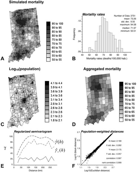
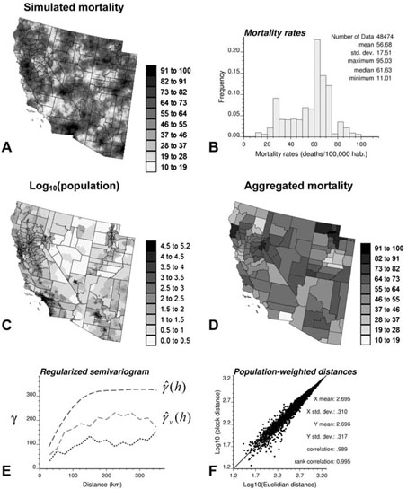
Figures 1A and 2A show one realization of the mortality variable for two contrasted county geographies: 1) state of Indiana that consists of 92 counties of fairly similar size and shape (Region 1), and 2) four states in the Western US (Arizona, California, Nevada and Utah) that form a set of 118 counties that are vastly different geographical units (Region 2). The two maps were generated by sequential Gaussian simulation using an isotropic spherical semivariogram model with no nugget effect and a range of 100 km for Region 1 and 150 km for Region 2. The histograms of simulated values reproduce the histograms of lung cancer mortality rates that were observed for white males over these same regions during the period 1970–1994 (Pickle et al. 1999). In Region 2, the distribution of data is strongly asymmetric and multimodal. This illustrates the applicability of the proposed methodology under non-normal situations. Simulated values are here used since it allows investigating the impact of spatial aggregation of the underlying punctual process, which is unknown in practice.

Fig. 1.

(A) Simulated mortality map (5 km resolution) in Indiana (Region 1). (B)Mortality rates in Indiana (Region 1). Accounting for the population density (C), mortality values are aggregated within each of the 92 counties (D). Bottom graph shows the omnidirectional semivariograms of mortality before ŷ(h)) and after (ŷ_ν(h)) aggregation, and their difference (E). The scattergram plots Euclidean distances between county centroids versus a “block distance” that accounts for the shape of counties and the distribution of the population (F).

Fig. 2.

(A) Simulated mortality map (5 km resolution) in four states of the Western US (Region 2). (B) Mortality rates in western US. Accounting for the population density (C), mortality values are aggregated within each of the 118 counties (D). Bottom graph shows the omnidirectional semivariograms of mortality before (ŷ(h)) and after (ŷ_ν(h)) aggregation, and their difference (E). The scattergram plots Euclidean distances between county centroids versus a ‘block distance’ that accounts for the shape of counties and the distribution of the population (F).

The spatial weight function for the aggregation of mortality values is the population maps displayed in Figs. 1C and 2C. The population in each 25 km² cell was retrieved by proportional allocation of the 2000 census block level data. These maps highlight the non-uniform distribution of population sizes within counties, a factor that will be incorporated in the analysis. Aggregated (i.e. county-level) mortality data were computed as the population-weighted average of mortality data for all cells falling within that county (Figs. 1D and 2D).

The spatial variability of the mortality variable before and after aggregation to the county level is quantified using the semivariogram. For the fine grid, the estimator of the ‘point support’ semivariogram is the traditional half mean squared difference of values separated by a given vector h

$$\widehat{\gamma }(\mathbf{\text{h}})=\frac{1}{2N(\mathbf{\text{h}})}{\displaystyle \underset{j=1}{\overset{N(\mathbf{\text{h}})}{\Sigma }}[z({\mathbf{\text{u}}}_j)}-z({\mathbf{\text{u}}}_j+{\mathbf{\text{h)]}}}^2\text{,}$$ 1

where z(u _j) is the mortality simulated at the grid node u _j referenced by the vector of spatial coordinates (x _j, y _j). The aggregation process leads to a smaller set of countylevel mortality data z(v_α). The semivariogram for the aggregated values (regularized or areal semivariogram) is estimated as

$${\widehat{\gamma }}_{\nu }(\mathbf{\text{h}})=\frac{1}{2N(\mathbf{\text{h}})}{\displaystyle \underset{\alpha =1}{\overset{N(\mathbf{\text{h}})}{\Sigma }}[z({\nu }_{\alpha })}-z({\nu }_{\alpha }+{\mathbf{\text{h)]}}}^2\text{.}$$ 2

The proximity between two polygons is typically measured by the Euclidean distance between their geographical centroids (Cressie 1993; Oliver et al. 1998; Christakos and Lai 1997; Christakos and Serre 2000; Berke 2004). To account for the shape of geographical units and their heterogeneous population density, the distance between any two counties is estimated as a population-weighted average of Euclidean distances between points discretizing the pair of counties

$$\text{Dist(}{\nu }_{\alpha }\text{, }{\nu }_{\beta }\text{) =}\frac{1}{{\displaystyle {\Sigma }_{s=1}^{P_{\alpha }}{\displaystyle {\Sigma }_{s^{\prime }=1}^{P_{\beta }}n({\mathbf{\text{u}}}_s)n({\mathbf{\text{u}}}_{s^{\prime }})}}}{\displaystyle \underset{s=1}{\overset{P_{\alpha }}{\Sigma }}{\displaystyle \underset{s^{\prime }=1}{\overset{P_{\beta }}{\Sigma }}n({\mathbf{\text{u}}}_s)n({\mathbf{\text{u}}}_{s^{\prime }})\parallel {\mathbf{\text{u}}}_s-{\mathbf{\text{u}}}_{s^{\prime }}\parallel }}\text{,}$$ 3

where P_α and P_β are the number of points u_s and u_s′ used to discretize the two units ν_α and ν_β, respectively. The quantity n(u_s) represents the population size within the 25 km² cell centred on the discretizing point u_s. For Figs. 1 and 2, the discretizing points are identified with the nodes of the 5 km simulation grid, yielding a total of 9 to 69 points per county in Indiana, and 11 to 2,082 discretizing points for the West Coast counties. The set of block-to-block distances (3) are plotted against the Euclidean distances between polygon centroids in Figs. 1F and 2F. Discrepancies between the two sets of distances are the largest for neighboring counties (i.e. for small distances). The correlation, albeit very high, is slightly smaller for Region 2, which is caused by the much larger heterogeneity of county shapes and sizes.

Figures 1E and 2E display the semivariograms of mortality data before and after aggregation, as well as their difference (dotted curve). As expected, the aggregation reduces the variability of the data, leading to semivariograms with smaller sills. However, unlike the assumption classically used in the geostatistical literature for distances larger than the size of geographical units (Journel and Huijbregts 1978; Armstrong 1998), the two semivariograms do not systematically differ by a constant. This is particularly obvious for Region 2 where the size of the counties, measured by the number of discretizing points, varies by two orders of magnitude. The smaller difference between semivariograms for short distances reflects the fact that smaller counties (blocks characterized by smaller within-block variability) tend to be paired at shorter distances. A new procedure that incorporates the shape, size and orientation of geographical units in the deconvolution procedure is needed. The ultimate objective is the mapping of the distribution of mortality within each county using solely the aggregated mortality data and their semivariogram. In other words, how do we estimate the maps of Figs. 1A and 2A if the only information available is the county-level maps (Figs. 1D, 2D) and the semivariogram of areal data?

3 Accounting for Spatial Support in Kriging

This section starts with a brief recall of the common centroid-based implementation of ordinary kriging for prediction of areal values. The approach is then modified to account for spatial supports and a spatial weight function (i.e. population density) in area-to-area and area-to-point predictions.

3.1 Point Kriging of Areal Data

Assume temporarily that all geographical units ν_α have similar shapes and sizes, with a uniform population density. These units can be referenced geographically by their centroids u_α = (x_α, y_α). The attribute z over a given unit ν_β is estimated as a linear combination of the z-data observed in K neighboring units

$${\widehat{z}}_{\text{OK}}({\mathbf{\text{u}}}_{\beta })={\displaystyle \underset{i=1}{\overset{K}{\Sigma }}{\text{λ}}_i({\mathbf{\text{u}}}_{\beta })z({\mathbf{\text{u}}}_i)}\text{,}$$ 4

where λ_i (u _β) is the weight assigned to z(u_i) for the prediction at u_β. The K weights are the solution of the following system of linear equations

$$\begin{array}{l}{\displaystyle \underset{j=1}{\overset{K}{\Sigma }}{\text{λ}}_j({\mathbf{\text{u}}}_{\beta })C({\mathbf{\text{u}}}_i-{\mathbf{\text{u}}}_j)+\mu ({\mathbf{\text{u}}}_{\beta })}=C({\mathbf{\text{u}}}_i-{\mathbf{\text{u}}}_{\beta }),i=1,\mathrm{...},K,\\ {\displaystyle \underset{j=1}{\overset{K}{\Sigma }}{\text{λ}}_j({\mathbf{\text{u}}}_{\beta })}=1.\end{array}$$ 5

Because of the exactitude property of kriging, the estimate ${\widehat{z}}_{\text{OK}}({\mathbf{\text{u}}}_{\beta })$ will be equal to the z-data z(u_i) whenever β = i. The prediction variance associated with the estimate (4) is computed using the traditional formula for the ordinary kriging variance

$${\sigma }_{\text{OK}}^2({\mathbf{\text{u}}}_{\beta })=C(0)-{\displaystyle \underset{i=1}{\overset{K}{\Sigma }}{\text{λ}}_i}({\mathbf{\text{u}}}_{\beta })C({\mathbf{\text{u}}}_i-{\mathbf{\text{u}}}_{\beta })-\mu ({\mathbf{\text{u}}}_{\beta })\text{.}$$ 6

To compute the kriging weights λ_i (u_β), the Lagrange multiplier μ(u_β), and kriging variance ${\sigma }_{OK}^2\left({\mathbf{u}}_{\beta }\right)$ one needs to know the point support covariance C(h), or equivalently the semivariogram γ(h) = C(0) − C(h) which can be estimated using an expression of type (1).

3.2 Area-to-Area (ATA) Kriging

In the situation where the geographical units have very different shapes and sizes, areal data cannot be simply collapsed into their respective polygon centroids. In Kyriakidis (2004), ATA kriging refers to the case where both the prediction and measurement supports are blocks instead of points. The OK estimate (4) for the areal value z(ν_β) becomes

$${\widehat{z}}_{OK}({\nu }_{\beta })={\displaystyle \sum _{i=1}^K{\lambda }_i({\nu }_{\beta })}z(v_i).$$ 7

The ordinary kriging system (5) is now written as

$$\begin{array}{l}{\displaystyle \underset{j=1}{\overset{K}{\Sigma }}{\text{λ}}_j({\nu }_{\beta })\overline{C}}({\nu }_i,{\nu }_j)+\mu ({\nu }_{\beta })=\overline{C}({\nu }_i,{\nu }_{\beta }),i=1,\mathrm{...},K,\\ {\displaystyle \underset{j=1}{\overset{K}{\Sigma }}{\text{λ}}_j({\nu }_{\beta })}=1\text{.}\end{array}$$ 8

The main change is that the K² point-to-point covariance terms C(u_i – u_j) are replaced by the block-to-block covariance term $\overline{C}({\nu }_i,{\nu }_j)=\text{Cov}\left\{Z({\nu }_i),Z({\nu }_j)\right\}\text{.}$ Similar to traditional block kriging, these covariances are approximated by the average of the point support covariance C(h), computed between any two points discretizing the blocks v_i and v _j

$$\overline{C}\left({\nu }_i,{\nu }_j\right)=\frac{1}{{\displaystyle {\sum }_{s=1}^{P_i}{\displaystyle {\sum }_{s^{\prime }=1}^{P_j}{w}_{s{s}^{\prime }}}}}{\displaystyle \sum _{s=1}^{P_i}{\displaystyle \sum _{s^{\prime }=1}^{P_j}{w}_{s{s}^{\prime }}C\left({\mathbf{\text{u}}}_s,{\mathbf{\text{\hspace{0.25em}u}}}_{s^{\prime }}\right),}}$$ 9

where P_i and P_j are the number of points used to discretize the two blocks ν_i and ν_j, respectively. The weights w_ss′ are computed as the product of individual weights (population sizes) assigned to the discretizing point u_s and u_s′

$$w_{s{s}^{\prime }}=n({\mathbf{u}}_s)\times n({\mathbf{u}}_{s^{\prime }})\text{\hspace{0.25em}with\hspace{0.25em}}{\displaystyle \sum _{s=1}^{P_i}n({\mathbf{u}}_s)}=n({\nu }_i)\text{\hspace{0.25em}and\hspace{0.25em}}{\displaystyle \sum _{s^{\prime }=1}^{P_j}n({\mathbf{u}}_{s^{\prime }})}=n({\nu }_j).$$ 10

The kriging variance for the areal estimator is computed as

$${\sigma }_{OK}^2(v_{\beta })=\overline{C}({\nu }_{\beta },{\nu }_{\beta })-{\displaystyle \sum _{i=1}^K{\lambda }_i(v_{\beta })\overline{C}}({\nu }_i,{\nu }_{\beta })-\mu ({\nu }_{\beta }),$$ 11

where $\overline{C}({\nu }_{\beta },{\nu }_{\beta })$ is the within-block covariance that is approximated using expression (9) with i = j = β.

3.3 Area-to-Point (ATP) Kriging

A major limitation of the choropleth maps is the common biased visual perception that larger areas are of greater importance. One solution is to create continuous maps of the attribute of interest, which amounts to performing a disaggregation or area-to-point interpolation. At each discretizing point u_s within an entity ν_β, the attribute value z(u_s) can be estimated as the following linear combination of areal data

$${\widehat{z}}_{OK}({\mathbf{u}}_s)={\displaystyle \underset{i=1}{\overset{K}{\Sigma }}{\lambda }_i({\mathbf{u}}_s)}z({\nu }_i).$$ 12

The kriging system is similar to system (8), except for the right-hand-side term where the block-to-block covariance $\overline{C}({\nu }_i,{\nu }_{\beta })$ is replaced by the block-to-point covariance $\overline{C}({\nu }_i,{\mathbf{\text{u}}}_s)\text{.}$ The latter is approximated by a procedure similar to the one described in (9) with P_j = 1. A critical property of the ATP kriging estimator is its coherence. The aggregation of the P_β point estimates within any given entity ν_β must yield the areal data z(ν_β)

$$z({\nu }_{\beta })=\frac{1}{n\left({\nu }_{\beta }\right)}{\displaystyle \underset{s=1}{\overset{P_{\beta }}{\Sigma }}n}({\mathbf{\text{u}}}_s){\widehat{z}}_{\text{OK}}({\mathbf{\text{u}}}_s)\text{.}$$ 13

Constraint (13) is satisfied if the same K areal data are used for the estimation of each of the P_β discretizing point u_s. In this case, the weighted average of the right-hand-side covariance terms of the K ATP kriging systems is equal to the right-hand-side covariance of the single ATA kriging system

$$\begin{array}{l}\frac{1}{n({\nu }_{\beta })}{\displaystyle \underset{s=1}{\overset{P_{\beta }}{\Sigma }}n({\mathbf{u}}_s)}\overline{C}({\nu }_i,{\mathbf{u}}_s)=\frac{1}{n({\nu }_{\beta })}{\displaystyle \underset{s=1}{\overset{P_{\beta }}{\Sigma }}n({\mathbf{u}}_s)}\left[\frac{1}{n({\nu }_i)}{\displaystyle \sum _{s^{\prime }=1}^{P_i}n({\mathbf{u}}_{s^{\prime }})C({\mathbf{u}}_{s^{\prime }},{\mathbf{u}}_s)}\right]\\ =\overline{C}({\nu }_i,{\nu }_{\beta }),\end{array}$$ 14

per relations (9) and (10). Therefore, the following relationship exists between the two sets of ATA and ATP kriging weights

$${\text{λ}}_i({\nu }_{\beta })=\frac{1}{n\left({\nu }_{\beta }\right)}{\displaystyle \underset{s=1}{\overset{P_{\beta }}{\Sigma }}n({\mathbf{\text{u}}}_s){\text{λ}}_i}({\mathbf{\text{u}}}_s),\mathrm{\hspace{0.25em}i}=1,\mathrm{...},K\text{.}$$ 15

The kriging variance for the ATP estimator is computed as

$${\sigma }_{\text{OK}}^2({\mathbf{\text{u}}}_s)=C(0)-{\displaystyle \underset{i=1}{\overset{K}{\Sigma }}{\text{λ}}_i}({\mathbf{\text{u}}}_s)\overline{C}({\nu }_i,{\mathbf{\text{u}}}_s)-\mu ({\mathbf{\text{u}}}_s)\text{.}$$ 16

4 Accounting for Spatial Support in Semivariogram Deconvolution

To implement both ATA and ATP kriging, one needs to know the point support covariance C(h), or equivalently the point support semivariogram γ(h). This section first introduces the analytical expression for the regularization of point support semivariograms in presence of regular blocks, and then it is generalized to the case of irregular geographical units. The new deconvolution procedure is then presented.

4.1 Regularization of the Point Support Semivariogram: Regular Geographical Units

Following Journel and Huijbregts (1978, p. 77), the point support and regularized semivariograms are related by the general formula

$$2{\gamma }_{\nu }(\mathbf{\text{h}})=2\overline{\gamma }\left(\nu (\mathbf{\text{u}}),\nu (\mathbf{\text{u+h)}}\right)-\overline{\gamma }\left(\nu (\mathbf{\text{u}}),\nu (\mathbf{\text{u}})\right)-\overline{\gamma }\left(\nu (\mathbf{\text{u+h}}),\nu (\mathbf{\text{u+h}})\right)$$ 17

which, under the assumption of stationarity, becomes

$${\gamma }_{\nu }(\mathbf{\text{h}})=\overline{\gamma }(\nu ,{\nu }_{\mathbf{\text{h}}})-\overline{\gamma }(\nu ,\nu )\text{.}$$ 18

The block-to-block semivariogram value $\overline{\gamma }(\nu ,{\nu }_{\mathbf{\text{h}}})$ represents the mean value of the point support semivariogram between an arbitrary point in the support ν and another in the translated support ν_h. The second term, $\overline{\gamma }(\nu ,\nu )$ is the within-block semivariogram value. For distances h = |h| that are very large in comparison with the dimension of the support ν, the following approximation is used in practice

$${\gamma }_{\nu }(\mathbf{\text{h}})=\gamma (\mathbf{\text{h}})-\overline{\gamma }(\nu ,\nu )\text{.}$$ 19

Equation (19) avoids the cumbersome estimation of the quantity $\overline{\gamma }(\nu ,{\nu }_{\mathbf{\text{h}}})$and was validated in case studies (Armstrong 1998, p. 80). The within-block semivariogram value is commonly estimated using the following arithmetical average

$$\overline{\gamma }(\nu ,\nu )=\frac{1}{P^2}{\displaystyle \underset{s=1}{\overset{P}{\Sigma }}{\displaystyle \underset{s^{\prime }=1}{\overset{P}{\Sigma }}\gamma ({\mathbf{\text{u}}}_s,{\mathbf{\text{u}}}_{s^{\prime }})\text{,}}}$$ 20

where P is the number of points used to discretize the block ν.

4.2 Regularization of the Point Support Semivariogram: Irregular Geographical Units

In addition to the assumption of stationarity, (18) is derived under the assumption that all the blocks in the study area have the same size and shape. Therefore, the within-block semivariogram value $\overline{\gamma }(\nu ,\nu )$ is constant. The following, more general, expression for the regularization is proposed

$${\gamma }_{\nu }(\mathbf{\text{h}})=\overline{\gamma }(\nu ,{\nu }_{\mathbf{\text{h}}})-{\overline{\gamma }}_{\mathbf{\text{h}}}(\nu ,\nu )\text{.}$$ 21

The within-block semivariogram value now varies as a function of the separation vector h, since the size of the blocks varies as a function of the distance between them. Smaller blocks tend to be paired at shorter distances, while larger blocks can only be paired for distances that exceed half their minimum dimension. This quantity is estimated as the arithmetical average of within-block semivariogram values for blocks separated by a given vector h

$${\overline{\gamma }}_{\mathbf{h}}\left(\nu ,\nu \right)=\frac{1}{2N(\mathbf{h})}{\displaystyle \underset{\alpha =1}{\overset{N(\mathbf{h})}{\Sigma }}\left[\overline{\gamma }\left({\nu }_{\alpha },{\nu }_{\alpha }\right)+\overline{\gamma }\left({\nu }_{\alpha +h},{\nu }_{\alpha +\mathbf{h}}\right)\right]},$$ 22

where $\overline{\gamma }({\nu }_{\alpha },{\nu }_{\alpha })$ and $\overline{\gamma }({\nu }_{\alpha +\mathbf{\text{h}}},{\nu }_{\alpha +\mathbf{\text{h}}})$are estimated according to (20), and h is computed according to (3). If all the blocks are the same, then $\overline{\gamma }({\nu }_{\alpha },{\nu }_{\alpha })=\overline{\gamma }({\nu }_{\alpha +\mathbf{\text{h}}},{\nu }_{\alpha +\mathbf{\text{h}}})\forall \mathbf{\text{h}}$and (22) is equal to the constant $\overline{\gamma }(\nu ,\nu )$Similarly, the first term $\overline{\gamma }(\nu ,{\nu }_{\mathbf{\text{h}}})$in (21) is estimated as

$$\overline{\gamma }\left(\nu ,{\nu }_{\mathbf{h}}\right)=\frac{1}{N(\mathbf{h})}{\displaystyle \underset{\alpha =1}{\overset{N(\mathbf{h})}{\Sigma }}\overline{\gamma }\left({\nu }_{\alpha },{\nu }_{\alpha +\mathbf{h}}\right)}.$$ 23

The semivariogram value between any two blocks, ν_α and ν_α+h, separated by h is computed as

$$\overline{\gamma }\left({\nu }_{\alpha },{\nu }_{\alpha +\mathbf{h}}\right)=\frac{1}{P_{\alpha }{P}_{\alpha +\mathbf{h}}}{\displaystyle \underset{s=1}{\overset{P_{\alpha }}{\Sigma }}{\displaystyle \underset{s^{\prime }=1}{\overset{P_{\alpha +\mathbf{h}}}{\Sigma }}\gamma \left({\mathbf{u}}_s,{\mathbf{u}}_{s^{\prime }}\right)},}$$ 24

where P_α and P_α+h are the number of points used to discretize the two blocks ν_α and ν_α+h, respectively.

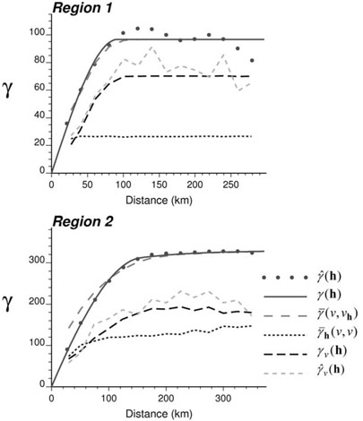
Expressions (21) through (24) were applied to the regularization of the semivariogram model fitted for the two simulated maps in Figs. 1A and 2A. The results displayed in Fig. 3 lead to the following comments:

Fig. 3.

Application of the regularization equation (21) to the point support semivariogram model γ(h) fitted to experimental values (black dots) for Regions 1 and 2. The theoretically regularized semivariogram model γ_ν(h), computed as the difference ${\gamma }_{\nu }(\mathbf{\text{h}})=\overline{\gamma }(\nu ,{\nu }_{\mathbf{\text{h}}})-{\overline{\gamma }}_{\mathbf{\text{h}}}(\nu ,\nu )$, is compared to the experimental semivariogram ${\widehat{\gamma }}_{\nu }(\mathbf{\text{h}})$ computed directly from areal data.

• The approximation $\overline{\gamma }(\nu ,{\nu }_{\mathbf{\text{h}}})\approx \gamma (\mathbf{\text{h}})$ is valid only for large distances, which confirms Journel and Huijbregts' statement that it should be used only for distances much larger than the dimension of the blocks. Assuming that all counties are square, the average block dimension is 32.4 km for Region 1 and 81.2 km for Region 2. In particular for Region 2, the use of the point support semivariogram causes an underestimation of the block-to-block semivariogram value at short distances.

• The within-block semivariogram value ${\overline{\gamma }}_{\mathbf{\text{h}}}(\nu ,\nu )$ is nearly constant $\forall h$ in Region 1 where all counties have fairly similar size and shape. For Region 2, the preferential pairing of small counties, with small within-block variance, for shorter distances causes an increase in ${\overline{\gamma }}_{\mathbf{\text{h}}}(\nu ,\nu )$ value as a function of the separation distance h.

• The regularized semivariogram model γ_ν (h) derived using expression (21) is reasonably close to the experimental semivariogram ${\widehat{\gamma }}_{\nu }(\mathbf{\text{h}})$ computed directly from areal data (2).

4.3 Deconvolution of the Regularized Semivariogram

The inference of a point support semivariogram from the semivariogram of areal data is not as straightforward as the regularization procedures described earlier. In mining applications, the data support is often very small with respect to the distance involved in the estimation, as well as the size of the blocks to be estimated (prediction support). In these cases, the support ν can be approximated to a quasi-point support (|ν| ≈ 0), and the experimental semivariogram of areal data ${\widehat{\gamma }}_{\nu }(\mathbf{\text{h}})$ can be treated as an estimator of the point support model γ(h) (Journel and Huijbregts 1978, p. 231). These assumptions are clearly unrealistic for applications in health and social sciences, where the blocks can be very large.

Like most inverse problems, the deconvolution is best tackled using an iterative procedure. Journel and Huijbregts (1978, p. 90) proposed the following general approach:

1. Define a point support model from inspection of the semivariogram of areal data ${\widehat{\gamma }}_{\nu }(\mathbf{\text{h}})$, and estimate the parameters (sill, range) using basic deconvolution rules (Journel and Huijbregts 1978, p. 270; Kupfersberger et al. 1998).

2. Compute the theoretically regularized model γ_ν(h) using approximation (19) and compare it with the experimental curve ${\widehat{\gamma }}_{\nu }(\mathbf{\text{h}})\text{.}$

3. Adjust the parameters of the point support model so as to bring the regularized model in line with ${\widehat{\gamma }}_{\nu }(\mathbf{\text{h}})\text{.}$

No recommendation was formulated regarding the way the parameters of the point support model should be adjusted or how to assess the closeness between the experimental and theoretically regularized semivariogram models. A similar approach was proposed in the remote sensing literature for deconvolution in the presence of regular pixels, yet the estimation of semivariogram parameters was not clearly discussed (Collins and Woodcock 1996, 1999). In this paper, the same paradigm is used to develop a deconvolution procedure that is fully automated and can accommodate geographical units of different sizes and shapes. The iterative approach proceeds as follows:

1. Compute the experimental semivariogram of areal data ${\widehat{\gamma }}_{\nu }(\mathbf{\text{h}})$ (2) and fit a model ${\gamma }_{\nu }^{\exp }(\mathbf{\text{h}})$ using weighted least-square regression (Pardo-Iguzquiza 1999). Three types of semivariogram model (spherical, exponential, and cubic) are tried and the one that yields the smallest deviation between the experimental and modeled curves is selected. Each lag is weighted by $\sqrt{N(\mathbf{\text{h}})}/{\gamma }_{\nu }^{\exp }(\mathbf{\text{h}})$to assign more importance to the fitting of semivariogram values at short distances.

2. As an initial point support model γ⁽⁰⁾(h), use the model (type of semivariogram function and parameters) fitted to areal data, ${\gamma }_{\nu }^{\exp }(\mathbf{\text{h}})$.

3. Regularize the model γ⁽⁰⁾(h) according to expression (21)

   $${\gamma }_{\nu }^{(0)}(\mathbf{\text{h}})={\overline{\gamma }}^{(0)}(\nu ,{\nu }_{\mathbf{\text{h}}})-{\overline{\gamma }}_{\mathbf{\text{h}}}^{(0)}(\nu ,\nu )\text{.}$$
4. Quantify the deviation between the ‘data-based’ $({\gamma }_{\nu }^{\exp }(\mathbf{\text{h}}))$ and the theoretically regularized $({\gamma }_{\nu }^{(0)}(\mathbf{\text{h}}))$ semivariogram models using the average relative difference between these two curves over L lags h_l

   $$D^{(0)}=\frac{1}{L}{\displaystyle \underset{l=1}{\overset{L}{\Sigma }}\frac{\left|{\gamma }_{\nu }^{(0)}({\mathbf{\text{h}}}_l)-{\gamma }_{\nu }^{\exp }({\mathbf{\text{h}}}_l)\right|}{{\gamma }_{\nu }^{\exp }({\mathbf{\text{h}}}_l).}}$$ 25
5. Consider the initial point support model γ⁽⁰⁾(h), the regularized model ${\gamma }_{\nu }^{(0)}(\mathbf{\text{h}})$, and the associated difference statistic D⁽⁰⁾ as ‘optimal’ at this stage

   $${\gamma }^{\text{opt}}(\mathbf{\text{h}})={\gamma }^{(0)}(\mathbf{\text{h}}),{\gamma }_{\nu }^{\text{opt}}(\mathbf{\text{h}})={\gamma }_{\nu }^{(0)}(\mathbf{\text{h}}),\text{and }{D}^{\text{opt}}=D^{(0)}\text{.}$$
6. For each lag h_l, compute experimental values for the new point support semivariogram through a rescaling of the optimal point support model γ^opt(h)

   $${\widehat{\gamma }}^{(1)}({\mathbf{\text{h}}}_l)={\gamma }^{\text{opt}}({\mathbf{\text{h}}}_l)\times w^{(1)}({\mathbf{\text{h}}}_l)\text{\hspace{0.25em}with }{w}^{(1)}{\mathbf{\text{(h}}}_l\text{) =1+}\frac{({\gamma }_{\nu }^{\exp }({\mathbf{\text{h}}}_l)-{\gamma }_{\nu }^{\text{opt}}({\mathbf{\text{h}}}_l))}{s_{\exp }^2\sqrt{\text{iter}}}\text{,}$$

   where $s_{\exp }^2$ is the sill of the model ${\gamma }_{\nu }^{\exp }(\mathbf{\text{h}})$ fitted to areal data, and the parameter ‘iter’ indicates the iteration number (iter = 1 at this stage). The rescaling coefficient w⁽¹⁾ (h_l) exceeds one, causing an increase in the value of the point support model, for lags where the regularization of the optimal model underestimates the model fitted to areal data, ${\gamma }_{\nu }^{\text{opt}}(\mathbf{\text{h}})<{\gamma }_{\nu }^{\exp }(\mathbf{\text{h}})$. Conversely, the value of the point support model is decreased (w⁽¹⁾ (h_l) < 1) for lags where its regularization overestimates the model fitted to areal data, ${\gamma }_{\nu }^{\text{exp}}(\mathbf{\text{h}})>{\gamma }_{\nu }^{\text{opt}}(\mathbf{\text{h}})$. The use of lagspecific rescaling coefficients provides enough flexibility to modify the initial shape of the point support semivariogram and makes the deconvolution insensitive to the initial solution adopted. The denominator $\sqrt{\text{iter}}$ causes a gradual attenuation of the magnitude of changes as the deconvolution proceeds.

7. Fit a model γ⁽¹⁾(h) to the rescaled values using weighted least-square regression (same procedure as in step 1).

8. Regularize the model γ⁽¹⁾(h) according to expression (21)

   $${\gamma }_{\nu }^{(1)}(\mathbf{\text{h}})={\overline{\gamma }}^{(1)}(\nu ,{\nu }_{\mathbf{\text{h}}})-{\overline{\gamma }}_{\mathbf{\text{h}}}^{(1)}(\nu ,\nu )\text{.}$$
9. Compute the difference statistic (25) for the new regularized model ${\gamma }_{\nu }^{(1)}(\mathbf{\text{h}})\text{.}$

   • If D⁽¹⁾ < D^opt, use the point support model γ⁽¹⁾(h) and the associated statistic D⁽¹⁾ as new optimum. Repeat steps 6 through 8.
   • If D⁽¹⁾ ≥ D^opt, repeat steps 6 through 8 using the same optimal model but the new rescaling coefficients computed as

     $$w^{(2)}({\mathbf{\text{h}}}_l)=1+\frac{(w^{(1)}({\mathbf{\text{h}}}_l)-1)}{2}\text{.}$$
     Each new coefficient w⁽²⁾(h_l) is the mid-point between the old coefficient w⁽¹⁾(h_l) and one, creating a new candidate point support model that is closer to the optimal model found so far.

10. Stop the iterative procedure after the i-th iteration whenever one of the following three criteria is met: (1) the difference statistic reaches a sufficiently small value; for example, D⁽ⁱ⁾ / D⁽⁰⁾ ≤ 0.05, or (2) the maximum number of allowed iterations has been tried; for example, iter > 25, or (3) a small decrease in the difference statistic D was recorded a given number of times; for example, |D⁽ⁱ⁾ − D^opt|/D^opt ≤ 0.01 was recorded three times.

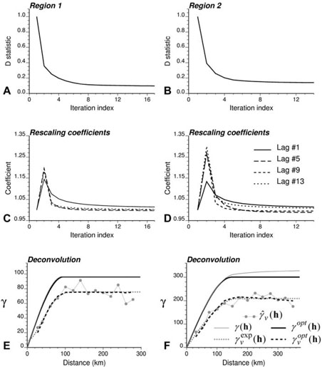
This iterative procedure was applied to the deconvolution of the regularized models in Figs. 1 and 2. Figures 4A and 4B shows that a few iterations substantially lowered the initial value of the difference statistic (25). For both regions, the procedure stopped once a small decrease (<1%) in the D statistic occurred three times, after 17 iterations for Region 1 and 14 iterations for Region 2. Figures 4C and 4D shows the corresponding evolution of the rescaling coefficients for a few lags. At the first iteration their value is one, since the initial optimum is the model fitted to areal data, ${\gamma }_{\nu }^{\text{opt}}(\mathbf{\text{h}})={\gamma }_{\nu }^{\exp }(\mathbf{\text{h}})$. As expected, the rescaling coefficients increase at the next iteration, since the values of the point support model are typically larger than the regularized semivariogram values. This increase is more pronounced for Region 2 and likely reflects the more complex impact of the heterogeneous county geography on the regularization process. From there, the values of all rescaling coefficients gently converge to one. For both regions, the decline is the slowest for the first lag which is also the part of the experimental regularized semivariogram that is not perfectly reproduced; see deviations between ${\gamma }_{\nu }^{\text{opt}}(\mathbf{\text{h}})\text{and }{\gamma }_{\nu }^{\exp }(\mathbf{\text{h}})$ in Figs. 4E and 4F. For Region 1, the deconvoluted model γ^opt(h) (black solid curve) almost perfectly matches the underlying point support model. The prediction of the point support model is also very good for Region 2, with only a slight underestimation of the semivariogram sill.

Fig. 4.

Application of the deconvolution procedure to the regularized semivariograms of Regions 1 and 2. As the iteration progresses, the lag-specific rescaling coefficients (C, D) converge to one while the D statistic (A, B), which measures the difference between the theoretically regularized model ${\gamma }_{\nu }^{\text{opt}}(\mathbf{\text{h}})$ and the experimental curve ${\gamma }_{\nu }^{\text{exp}}(\mathbf{\text{h}})$, declines. In both regions (E, F) the deconvoluted model γ^opt(h) is reasonably close to the “true” point support model γ (h).

5 Performance Assessment of Deconvolution and ATP Kriging

The performance of the deconvolution procedure and the area-to-point kriging was investigated using a set of simulated mortality maps over Regions 1 and 2. The impact of the following factors is explored: the range of autocorrelation of the underlying process, the spatial resolution of the discretizing grid, and the prediction errors of ATP kriging versus a simplistic kriging of centroids-based areal data.

5.1 Simulation of Mortality Values

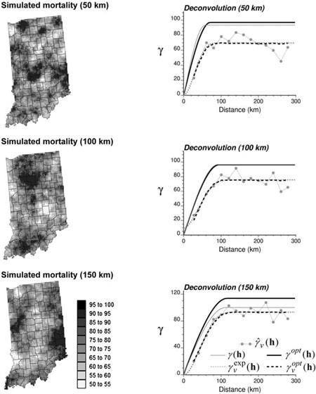
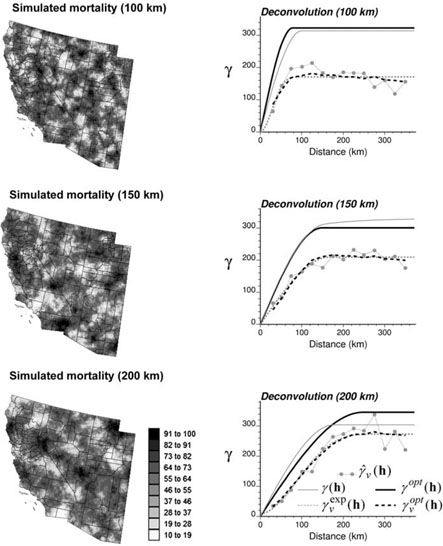
Simulated mortality maps were generated using sequential Gaussian simulation. The simulation grid, which has a 5 km spacing, consists of N = 3,751 and N = 48,474 nodes for Regions 1 and 2, respectively. The simulation was conditioned to the histogram of lung cancer mortality rates observed for white males over these same regions during the period 1970–1994. Three spherical semivariogram models with no nugget effect and increasing ranges of autocorrelation were selected for each study area: 50 km, 100 km, and 150 km for Region 1; 100 km, 150 km, and 200 km for Region 2. One realization was generated for each type of spherical model. The set of three simulated maps for each region are displayed in Figs. 5 and 6 (left column). Different seeds for the random number generator (Deutsch and Journel 1998, p. 173) were used, so that high and low values do not appear at the same locations on the three simulated maps. The corresponding point support semivariograms were computed and a model γ (h) was automatically fitted using weighted least-square regression; see the top gray solid line in Figs. 5 and 6 (right column). This model is used as the target point support model in order to account for ergodic fluctuations that might cause the imperfect reproduction of the semivariogram model used in the simulation (Goovaerts 1997, p. 426).

Fig. 5.

Mortality simulated in Region 1 using three spherical models with no nugget effect and increasing ranges. Right column shows the results of the deconvolution. In all cases, the deconvoluted model γ^opt(h) is reasonably close to the “true” point support model γ (h). The similarity of the theoretically regularized model ${\gamma }_{\nu }^{\text{opt}}(\mathbf{\text{h}})$ and the experimental curve ${\gamma }_{\nu }^{\text{exp}}(\mathbf{\text{h}})$ illustrates the ability of the iterative procedure to achieve a solution.

Fig. 6.

Mortality simulated in Region 2 using three spherical models with no nugget effect and increasing ranges. Right column shows the results of the deconvolution. In all cases, the deconvoluted model γ^opt(h) is reasonably close to the “true” point support model γ (h). The similarity of the theoretically regularized model ${\gamma }_{\nu }^{\text{opt}}(\mathbf{\text{h}})$ and the experimental curve ${\gamma }_{\nu }^{\text{exp}}(\mathbf{\text{h}})$ illustrates the ability of the iterative procedure to achieve a solution.

5.2 Semivariogram Deconvolution

Each simulated map was aggregated to the county level using the spatial weight function (population maps) of Figs. 1C and 2C. Figures 1D and 2D show the results obtained for the middle range case: 100 km for Region 1 and 150 km for Region 2. The semivariogram of aggregated data was computed using expression (2) and a model ${\gamma }_{\nu }^{\text{exp}}(\mathbf{\text{h}})$was automatically fitted using weighted least-square regression; see the bottom gray dashed line in Figs. 5 and 6 (right column). In both regions, the difference between the sills of the point support (γ (h)) and areal ${\gamma }_{\nu }^{\text{exp}}(\mathbf{\text{h}})$) semivariogram models decreases as the range of autocorrelation increases. This trend is expected, since the impact of aggregation (reduction in the sample variance and symmetrization of the histogram) decreases as the spatial pattern becomes more continuous (Isaaks and Srivastava 1989, p. 465).

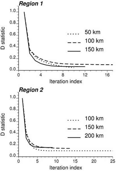
The deconvolution procedure was applied to each of the 6 regularized semivariograms. The evolution of the D statistic for each case is plotted in Fig. 7. The D statistic was standardized by its initial value D⁽⁰⁾ so that all curves start at one. For Region 1 the procedure always stopped once a small decrease (<1%) in the D statistic occurred three times, which happened after 10 to 17 iterations. For Region 2, the deconvolution required 9 and 14 iterations for two maps, and the limit of 25 iterations was reached for the simulated map with a range of 100 km. The final value of the D statistic is systematically lower for Region 1 due to the more homogeneous size and shape of the counties. The theoretically regularized semivariogram model γ_ν(h) (black dashed line in Figs. 5 and 6) shows a fairly good agreement with the ‘data-based’ model ${\gamma }_{\nu }^{\text{exp}}(\mathbf{\text{h}})$ for all situations.

Fig. 7.

Evolution of the D statistic during the iterative procedure of deconvolution for three different spatial patterns (spherical semivariogram models with increasing range) in Regions 1 and 2.

The final check is to compare the deconvoluted semivariogram model with the model fitted directly to the original simulated maps. Comparison of the top gray and black solid curves in Figs. 5 and 6 (right column) indicates that the deconvolution yields point support models that are reasonably close to the underlying ones. Because of the good agreement between theoretically regularized and ‘data-based’ semivariogram models, discrepancies at the point support level are essentially caused by the use of the regularization formula (21). An important factor that influences the deconvolution results is the behavior at the origin of the regularized and point support semivariogram models; for example, the fitting of a nugget effect or the use of a spherical (linear behavior) versus the cubic (parabolic behavior) model. In the absence of point data, this part of the semivariogram model can not be validated. No nugget effect was systematically fitted to the point support model to account for the characteristics of the model used in the simulation.

5.3 Impact of the Spatial Resolution of the Discretizing Grid

The deconvolution procedure can become very CPU intensive depending on the discretizing level adopted for the blocks. For the examples of Fig. 4, the CPU time on a Pentium 3.12 GHz (2048 MB RAM) was 22.3 seconds for Region 1 and 1,200 seconds for Region 2. The CPU time could be reduced by using less stringent stopping criteria. Using one instead of three small declines in the value of the D statistic for stopping the iterative procedure, this yields CPU times of 20.1 seconds for Region 1 and 953 seconds for Region 2. This faster procedure has minimal impact on the inference of the deconvoluted model.

In the presence of regular blocks, the computation is greatly facilitated by the fact that the within-block semivariogram term $\overline{\gamma }(\nu ,\nu )$ is the same for all blocks, while the block-to-block semivariogram term $\overline{\gamma }(\nu ,{\nu }_{\mathbf{\text{h}}})$ depends only on the separation vector h. For the geographies considered in this paper, these different terms must be computed for each block or possible pair of blocks since the counties are all different (expressions (22) and (23)). Whenever the shortest distance between discretizing points belonging to two different blocks exceeds the range of the point support semivariogram model, the block-to-block semivariogram term equals the sill for bounded models (spherical or cubic). Therefore, the computation of the $\overline{\gamma }(\nu ,{\nu }_{\mathbf{\text{h}}})$ term can be somewhat alleviated.

When the block sizes differ by several orders of magnitude as in Region 2, it is not computationally efficient to use the same discretizing level for each block. One solution is to use flexible discretizing grids that ensure a constant number of discretizing points within each block; this option is available in the deconvolution module of TerraSeer's STIS software (Avruskin et al. 2004). This paper explored the more straightforward alternative of using regular discretizing grids of coarser resolution. For Region 2, the deconvolution was conducted using 10 and 20 km discretizing grids including 12,129 and 3,037 nodes, respectively. At 10 km resolution, the number of discretizing points per county varies from 5 to 522, while the range is 1 to 129 for the coarsest grid. In the later case, if no grid node falls within a county, the population-weighted centroid of that county was used as single discretizing point for the computation of the block-to-block semivariogram term $\overline{\gamma }(\nu ,{\nu }_{\mathbf{\text{h}}})$. To calculate the within-block semivariogram term $\overline{\gamma }(\nu ,\nu )$, these small counties were assimilated to 400 km² squares (the smallest grid cell size) which were discretized using a 5 × 5 regular grid. Using coarser grids substantially reduces the initial CPU time of 1,200 seconds: 92.9 seconds for the 10 km grid and 9.4 seconds for the 20 km grid.

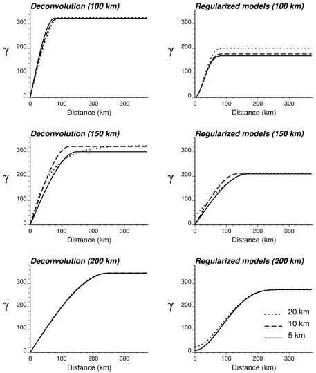
The impact of the discretizing level on the derivation of the optimal point support model is illustrated in Fig. 8 (left column). Differences between deconvoluted models essentially reflect differences between models fitted to regularized semivariograms (Fig. 8, right column) whose reproduction guides the iterative procedure. The largest differences were observed for the 150 km semivariogram model: the fitting of different types of regularized model (with or without the nugget effect) and changes in the range values translate into deconvoluted models that differ both in terms of sill and range. The deconvolution process appears less sensitive to differences in the sill of the regularized model (1st case of 100 km range). In all cases, discrepancies are of a small magnitude though.

Fig. 8.

Impact of the spatial resolution of the discretizing grid (i.e., 5, 10, or 20 km spacing grid) on the model fitted to the semivariogram of areal data (right column) and the results of the deconvolution (left column). The analysis was conducted for the three simulated maps of Region 2, using ranges of autocorrelation equal to 100, 150, and 200 km.

5.4 Prediction Performances of Area-to-Point Kriging

Deconvolution of the areal semivariogram is not a goal per se, but rather an intermediate step towards the mapping of the distribution of attribute values within each block. The prediction performance of ATP kriging was investigated for the sets of simulated maps of Regions 1 and 2. Performance criteria include the smoothing effect of kriging, the prediction bias, and the mean absolute error (MAE) of prediction between the 5 km simulated grid of reference values, and the grid of ATP kriging estimates. To assess the impact of the deconvoluted semivariogram model on the prediction, the same criteria were also computed for ATP kriging using the ‘true’ point support semivariogram model that was inferred directly from the simulated mortality maps (top gray solid curve in Figs. 5 and 6, right column). Finally, the naïve approach whereby centroid-based areal data are interpolated to the nodes of the regular grid using point kriging and the regularized semivariogram was also implemented.

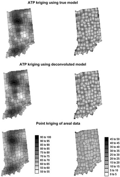
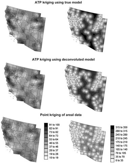
Figures 9 and 10 show the maps of kriging estimates and variances computed using the three alternative interpolation methods and the aggregated mortality maps of Figs. 1D and 2D. Unlike the point kriging of aggregated values, the two forms of ATP kriging ensure that within each county the population-weighted average of mortality estimates equals the areal data for that county. Visual inspection of the maps suggests that this coherence constraint attenuates the smoothness of kriging, leading to more details in the maps. Table 1 confirms that the variance of ATP kriging estimates, although smaller than the variance of reference simulated values, systematically exceeds the variance of point kriging estimates.

Fig. 9.

Maps of kriging estimates (left) and variances (right) computed for the 100 km range spatial pattern in Region 1 using three alternative interpolation methods: ATP kriging using true point support model γ(h), ATP kriging using deconvoluted model, and point kriging of areal data.

Fig. 10.

Maps of kriging estimates (left) and variances (right) computed for the 150 km range spatial pattern in Region 2 using three alternative interpolation methods: ATP kriging using true point support model γ(h), ATP kriging using deconvoluted model, and point kriging of areal data.

Table 1.

Variance of mortality estimates for three types of spatial pattern in Regions 1 and 2 and three alternative kriging approaches: ATP kriging with true (γ(h)) or deconvoluted (γ^opt(h)) semivariogram model, and point kriging of areal data

	ATP kriging using γ(h)	ATP kriging using γopt(h)	Point kriging of areal data	Variance of simulated values
Region 1
50 km	65.04	64.83	57.11	90.81
100 km	73.89	73.85	55.67	91.20
150 km	78.01	77.96	72.96	91.23
Region 2
100 km	73.67	61.69	33.63	311.0
150 km	133.3	128.1	87.53	306.4
200 km	161.0	174.6	146.3	298.7

Not only does ATP kriging increase the level of detail in the maps, but it also leads to more accurate predictions, as measured by the mean absolute error (MAE) of prediction in Table 2. The benefit of ATP kriging over point kriging is even more apparent when the statistic is population-weighted, assigning larger weight to mortality estimated in more densely populated areas. The largest MAE difference between methods is observed for the two cases (100 km range for both Regions 1 and 2) where the smoothing effect of point kriging is the most pronounced. Table 3 confirms that the coherence constraint is correctly implemented, since the population-weighted mean error of prediction is zero for ATP kriging. A small bias is observed when the same weight is assigned to all predictions. For all the statistics, the two forms of ATP kriging yield very similar results, which confirm the robustness of kriging with respect to small differences in the point support semivariogram model.

Table 2.

Population-weighted mean absolute error of prediction $\left|\widehat{z}(\mathbf{\text{u}})-z(\mathbf{\text{u}})\right|$ for three types of spatial pattern in Regions 1 and 2 and three alternative kriging approaches: ATP kriging with true (γ (h)) or deconvoluted (γ^opt(h)) semivariogram model, and point kriging of areal data. Numbers in parenthesis are the equally-weighted statistics

	ATP kriging using γ (h)	ATP kriging using γopt (h)	Point kriging of areal date
Region 1
50 km	3.909 (4.457)	3.951 (4.513)	4.069 (4.635)
100 km	3.005 (3.591)	3.005 (3.591)	3.947 (4.045)
150 km	2.551 (2.934)	2.548 (2.933)	2.696 (2.982)
Region 2
100 km	6.799 (12.394)	6.993 (12.510)	9.038 (13.192)
150 km	5.940 (10.998)	5.994 (10.999)	7.556 (11.602)
200 km	6.535 (9.526)	6.384 (9.749)	7.903 (11.020)

Table 3.

Population-weighted mean error of prediction $(\widehat{z}(\mathbf{\text{u}})-z(\mathbf{\text{u}}))$ for three types of spatial pattern in Regions 1 and 2 and three alternative kriging approaches: ATP kriging with true (γ(h)) or deconvoluted (γ^opt(h)) semivariogram model, and point kriging of areal data. Numbers in parenthesis are the equallyweighted statistics

	ATP kriging using γ (h)	ATP kriging using γopt (h)	Point kriging of areal data
Region 1
50 km	0.0 (0.106)	0.0 (0.098)	0.279 (0.133)
100 km	0.0 (0.110)	0.0 (0.107)	0.415 (−0.091)
150 km	0.0 (0.136)	0.0 (0.138)	−0.078 (0.058)
Region 2
100 km	0.001 (–0.746)	0.001 (–0.930)	–1.115 (0.107)
150 km	0.003 (–0.707)	0.003 (–0.957)	0.717 (–1.497)
200 km	0.002 (–0.090)	0.002 (–0.405)	–1.721 (0.193)

Differences between ATP and point kriging are much more pronounced in terms of prediction variance than estimated value. While the point kriging variance is mainly influenced by the location of county centroids (data geometry), the ATP kriging variance accounted for the spatial distribution of the population. The ATP variance increases in sparsely populated areas. This effect is particularly apparent in Region 2; compare the top right map in Fig. 10 with the population map of Fig. 2. The map of point kriging variance tends to be smoother than the map of ATP kriging variance, particularly when the counties have similar shape and size (similar data configuration) like in Indiana; compare the middle and bottom right-hand maps in Fig. 9. The smoothing effect is further enhanced by the nugget effect displayed by the areal semivariogram model for Region 1.

6 Conclusions

The analysis of health data and putative covariates, such as environmental, socioeconomic, behavioral, or demographic factors, is a promising application for geostatistics. It presents, however, several methodological challenges, since data are typically aggregated over irregular spatial supports and, in the case of health data, they often consist of a numerator and a denominator (i.e. population size). Whereas the first analytical developments of kriging clearly demonstrated its ability to accommodate different measurement and prediction supports, geostatistical prediction of irregular blocks has rarely been implemented, mainly because of its lack of application in mining. Thanks to the joint advances of GIS software and computational resources, one can move beyond the simplified regularization formula adopted in the early days of geostatistics, and generalize kriging and deconvolution methods to the complex geographies encountered in social and health sciences.

Capitalizing on recent work in the arena of change of support, this paper reformulated the area-to-point kriging system to incorporate not only the shape and size of geographical units, but also the spatial repartition of population within these units. The coherence constraint thus becomes that the population-weighted average of kriged estimates within each geographical unit equals the areal data for that unit. All developments in this paper were given for ordinary kriging, yet similar expressions can be developed for simple kriging that is the core of most stochastic simulation algorithms. Simulation studies showed that ATP kriging yields more accurate and detailed (less smoothness) prediction than a naïve point kriging of areal data where all counties are simply collapsed into their respective polygon centroids. Although point estimates might not seem reasonable in this context and the comparison is somewhat unfair, it is worth using as yardstick a straightforward method that is used very often by non-expert users to conduct disaggregation of areal data (Croner and De Cola 2001; Berke 2004).

Adoption of ATP kriging by the GIS community still faces the hurdle of inferring the point support semivariogram from the semivariogram of areal data. This paper introduced an iterative procedure that allows such an inference in the absence of any multi-Gaussian assumption (Kyriakidis 2004). This empirical approach is based on a generalization of the regularization formula to account for irregular blocks and a heterogeneous population density. It also automates the heuristic approach proposed by Journel and Huijbregts (1978), whereby the user was advised to manually modify the parameters of the point support model until its regularization is close to the model fitted to areal data. The method was demonstrated for isotropic singlestructure semivariogram models, yet it is very flexible and has been implemented for nested anisotropic models in the deconvolution module of TerraSeer's STIS software (Avruskin et al. 2004). This module also allows the specification of any semivariogram model as an initial solution in the iterative procedure. Although the sill of the semivariogram fitted to areal data is certainly smaller than the sill of the pointsupport model, this initial solution was found to be the best suited for an automatic implementation of the deconvolution algorithm. The use of classic dispersion variance calculations (Journel and Huijbregts 1978, p. 270; Kupfersberger et al. 1998) was very sensitive to the behavior at the origin of the semivariogram and, in particular for cubic structures, could lead to initial models with unrealistically high sills. The proposed correction of the range parameter was not suited for blocks of various sizes and irregular shapes.

Simulation studies conducted so far demonstrated that the iterative approach achieves a reasonable solution: theoretically regularized semivariogram models are usually very close to the ‘data-based’ model. Comparison of the deconvoluted model with the true point support model also demonstrated the merits of the new procedure. The main factor that affects deconvolution results is the behavior at the origin of the regularized and point support semivariogram models; behavior that cannot be inferred from the data available in practice. An exact identification of the point support model is illusory, as already stated by Journel and Huijbregts (1978, p. 231): “These techniques should not be used to deduce a point model which is illusively detailed … To be rigorous, it is not possible to reach a greater degree of precision than that of the smallest support v of the data without introducing supplementary and unverifiable hypothesis.” Deconvolution is an inverse problem and as such there are multiple point-support models that, once regularized, will yield the model fitted to areal data. The choice of a particular model can be left to the deconvolution algorithm or the geostatistician can narrow down the set of solutions based on his knowledge of the phenomenon under study. It is the approach I adopted in this paper by setting the nugget effect to zero. Fortunately, simulation studies confirmed the robustness of kriging with respect to small misspecifications of the semivariogram model. This result further supports the use of ATP kriging with a point support model that can never be fully validated over a naïve point kriging based on a semivariogram inferred under the very simplistic assumption of quasi-point support of areal data.

A major limitation of choropleth maps is the common biased visual perception that larger rural and sparsely populated areas are of greater importance. The approach presented in this paper allows the continuous mapping of attribute values, while accounting locally for population density and areal data through the coherence constraint. This form of kriging also facilitates the analysis of relationships between health data and putative covariates that are typically measured over different spatial supports. The extension of the proposed methodology to much larger datasets (thousands of census blocks) will be hampered by the large computational time resulting from the current use of uniform discretizing grids across the study area. Sensitivity analysis, however, indicated that the minor changes in the deconvoluted model caused by the use of coarser discretizing grids bear little consequences on the kriging predictions. Further research should investigate the implementation of flexible discretizing grids, as well as spectral methods for the fast inference of block-to-block and block-to-point semivariogram values.

References

- Armstrong M. Basic linear geostatistics. Springer, Berlin: 1998. p. 172. [Google Scholar]
- Avruskin GA, Jacquez GM, Meliker JR, Slotnick MJ, Kaufmann AM, Nriagu JO. Visualization and exploratory analysis of epidemiologic data using a novel space time information system. Int J Health Geogr. 2004;3(26) doi: 10.1186/1476-072X-3-26. doi:10.1186/1476-072X-3-26. [DOI] [PMC free article] [PubMed] [Google Scholar]
- Barabás N, Goovaerts P, Adriaens P. Geostatistical assessment and validation of uncertainty for three-dimensional dioxin data from sediments in an estuarine river. Environ Sci Technol. 2001;35(16):3294–3301. doi: 10.1021/es010568n. [DOI] [PubMed] [Google Scholar]
- Berke O. Exploratory disease mapping: kriging the spatial risk function from regional count data. Int J Health Geogr. 2004;3(18) doi: 10.1186/1476-072X-3-18. doi:10.1186/1476-072X-3-18. [DOI] [PMC free article] [PubMed] [Google Scholar]
- Chiles JP, Delfiner P. Geostatistics: modeling spatial uncertainty. Wiley, New York: 1999. p. 720. [Google Scholar]
- Christakos G, Lai J. A study of the breast cancer dynamics in North Carolina. Soc Sci Med. 1997;45(10):1503–1517. doi: 10.1016/s0277-9536(97)00080-4. [DOI] [PubMed] [Google Scholar]
- Christakos G, Serre ML. Spatiotemporal analysis of environmental exposure-health effect associations. J Expo Anal Environ Epidemiol. 2000;10(2):168–187. doi: 10.1038/sj.jea.7500077. [DOI] [PubMed] [Google Scholar]
- Collins JB, Woodcock CE. Explicit consideration of multiple landscape scales while selecting spatial resolutions. In: Mowrer HT, Czaplewski RL, Hamre RH, editors. Spatial accuracy assessment in natural resources and environmental sciences: second international symposium. Technical report RMGTR-277, United States department of Agriculture; Fort Collins, Colorado: 1996. pp. 121–128. [Google Scholar]
- Collins JB, Woodcock CE. Geostatistical estimation of resolution-dependent variance in remotely sensed images. Photogramm Eng Remote Sensing. 1999;65(1):41–50. [Google Scholar]
- Cressie N. Statistics for spatial data. Wiley, New York: 1993. p. 900. [Google Scholar]
- Croner CM, De Cola L. 2001 Visualization of disease surveillance data with geostatistics. Presented at UNECE (United Nations Economic Commission for Europe) work session on methodological issues involving integration of statistics and geography, Sept 2001, Tallinn. http://www.unece.org/ stats/documents/2001/09/gis/25.e.pdf.
- Curran PJ, Atkinson PM. Issues of scale and optimal pixel size. In: Stein A, van der Meer F, Gorte B, editors. Spatial statistics for remote sensing. Kluwer Academic, Dordrecht: 1999. pp. 115–133. [Google Scholar]
- Deutsch CV, Journel AG. GSLIB: Geostatistical software library and user's guide. 2nd. Oxford University Press; New York: 1998. p. 369. [Google Scholar]
- Goovaerts P. Geostatistics for natural resources evaluation. Oxford University Press; New York: 1997. p. 483. [Google Scholar]
- Goovaerts P. Geostatistical analysis of disease data: estimation of cancer mortality risk from empirical frequencies using Poisson kriging. Int J Health Geogr. 2005;4(31) doi: 10.1186/1476-072X-4-31. doi:10.1186/1476-072X-4-31. [DOI] [PMC free article] [PubMed] [Google Scholar]
- Goovaerts P. Geostatistical analysis of disease data: accounting for spatial support and population density in the isopleth mapping of cancer mortality risk using area-to-point Poisson kriging. Int J Health Geogr. 2006;5(52) doi: 10.1186/1476-072X-5-52. doi:10.1186/1476-072X-5-52. [DOI] [PMC free article] [PubMed] [Google Scholar]
- Goovaerts P, Jacquez GM, Greiling D. Exploring scale-dependent correlations between cancer mortality rates using factorial kriging and population-weighted semivariograms: a simulation study. Geogr Anal. 2005;37(2):152–182. doi: 10.1111/j.1538-4632.2005.00634.x. [DOI] [PMC free article] [PubMed] [Google Scholar]
- Gotway CA, Young LJ. Combining incompatible spatial data. J Am Stat Assoc. 2002;97(459):632–648. [Google Scholar]
- Gotway CA, Young LJ. A geostatistical approach to linking geographically-aggregated data from different sources. Technical report # 2004-012, Department of Statistics, University of Florida; 2004. [Google Scholar]
- Change of support: an inter-disciplinary challenge. In: Gotway CA, Young LJ, editors; Renard Ph, Demougeot-Renard H, Froidevaux R., editors. geoENV V—Geostatistics for Environmental Applications. Springer, Berlin: 2005. pp. 1–13. [Google Scholar]
- Houlding S. Direct volume estimation—a geostatistical technique for mine planning and grade control. Comput Geosci. 1999;25(10):1113–1123. [Google Scholar]
- Isaaks EH, Srivastava RM. An introduction to applied geostatistics. Oxford University Press; New York: 1989. p. 561. [Google Scholar]
- Journel AG, Huijbregts CJ. Mining geostatistics. Academic Press; London: 1978. p. 600. [Google Scholar]
- Kelsall J, Wakefield J. Modeling spatial variation in disease risk: a geostatistical approach. J Am Stat Assoc. 2002;97(459):692–701. [Google Scholar]
- Kupfersberger H, Deutsch CV, Journel AG. Deriving constraints on small-scale variograms due to variograms of large-scale data. Math Geol. 1998;30(7):837–852. [Google Scholar]
- Kyriakidis P. A geostatistical framework for area-to-point spatial interpolation. Geogr Anal. 2004;36(2):259–289. [Google Scholar]
- Mockus A. Estimating dependencies from spatial averages. J Comput Graph Stat. 1998;7(4):501–513. [Google Scholar]
- Monestiez P, Dubroca L, Bonnin E, Durbec JP, Guinet C. Geostatistical modelling of spatial distribution of Balenoptera physalus in the Northwestern Mediterranean Sea from sparse count data and heterogeneous observation efforts. Ecol Model. 2006;193(3–4):615–628. [Google Scholar]
- Oliver MA, Webster R, Lajaunie C, Muir KR, Parkes SE, Cameron AH, Stevens MCG, Mann JR. Binomial cokriging for estimating and mapping the risk of childhood cancer. IMA J Math Appl Med Biol. 1998;15(3):279–297. [PubMed] [Google Scholar]
- Pardo-Iguzquiza E. VARFIT: a Fortran-77 program for fitting variogram models by weighted least squares. Comput Geosci. 1999;25(3):251–261. [Google Scholar]
- Pickle LW, Mungiole M, Jones GK, White AA. Exploring spatial patterns of mortality: the new Atlas of United States mortality. Stat Med. 1999;18(23):3211–3220. doi: 10.1002/(sici)1097-0258(19991215)18:23<3211::aid-sim311>3.0.co;2-q. [DOI] [PubMed] [Google Scholar]