An Augmented Data Method for the Analysis of Nosocomial Infection Data

Abstract

The analysis of nosocomial infection data for communicable pathogens is complicated by two facts. First, typical pathogens more commonly cause asymptomatic colonization than overt disease, so transmission can be only imperfectly observed through a sequence of surveillance swabs, which themselves have imperfect sensitivity. Any given set of swab results can therefore be consistent with many different patterns of transmission. Second, data are often highly dependent: the colonization status of one patient affects the risk for others, and, in some wards, repeated admissions are common. Here, the authors present a method for analyzing typical nosocomial infection data consisting of results from arbitrarily timed screening swabs that overcomes these problems and enables simultaneous estimation of transmission and importation parameters, duration of colonization, swab sensitivity, and ward- and patient-level covariates. The method accounts for dependencies by using a mechanistic stochastic transmission model, and it allows for uncertainty in the data by imputing the imperfectly observed colonization status of patients over repeated admissions. The approach uses a Markov chain Monte Carlo algorithm, allowing inference within a Bayesian framework. The method is applied to illustrative data from an interrupted time-series study of vancomycin-resistant enterococci transmission in a hematology ward.

When patient-to-patient transmission is important, analyses of nosocomial infection data should account for dependencies caused by the fact that the risk for one person depends on the number of others who are infected. The importance of accounting for such dependencies has been widely appreciated for community pathogens (1) but only recently recognized in the hospital infection literature (2, 3). Longer-term temporal dependencies can be caused by repeated admissions of the same patients, and these readmissions can have profound implications for infection dynamics in health care settings (4–7). In some settings, such dependencies also need to be accounted for in the analysis.

A second complication arises from the fact that most hospital pathogens are bacteria frequently carried asymptomatically. At best, hospital transmission is only imperfectly observed by taking screening swabs from patients. In most clinical settings, such swabs are taken rarely (if at all). Imperfect sensitivity of these swabs further adds to the uncertainty.

One simple approach that has been used to assess factors associated with the transmission of nosocomial pathogens is to attempt to identify the times, and sometimes also the sources, of transmission events and relate them to the ward- and patient-level factors of interest (such as isolation precautions, colonization pressure, intervention phase of a study) (8–11). A limitation of such approaches is the need for arbitrary assumptions. For example, transmission is often assumed to occur at the midpoint between consecutive negative and positive screening swabs, and methods of determining sources of transmission range from taking the closest possible source patient (10) to making subjective assessments based on temporal, geographic, and staffing data (8).

Accurately identifying transmission events is itself a problem. Typically, authors assume that patients found to be carrying a pathogen within 48 hours of admission are colonized on admission, while pathogens first identified after this period are taken to be true acquisitions. Such arbitrary divisions have the virtue of being pragmatic and easily applied and have undoubtedly been useful, but they may also lead to systematic distortions: true transmission events occurring within the first 2 days of admission will be misclassified as importations from the community, and true importations with initial false-negative screening swabs will be misclassified as transmission events.

In this paper, it is shown that such arbitrary assumptions are not required. A method of analyzing typical hospital surveillance data resulting from patient screening swabs is presented. This method accounts for dependencies in the data and avoids the need for arbitrary assumptions about transmission routes and events by adopting a data augmentation approach. The augmented data combine the original data and the additional information needed to fully define a possible realization of the epidemic process. Each feasible set of values for the augmented data corresponds to one possible realization. Inferences are made by numerically integrating over all realizations of the augmented data consistent with the observed data. By this means, the method can accommodate uncertainties in the transmission times and pathways and in the admission and readmission colonization status of patients, and it allows for inherent uncertainties in the screening results. The approach extends recent methodological developments by simultaneously allowing for imperfect screening sensitivity, incorporating ward- and patient-level covariates, and, by explicitly modeling the loss or acquisition of colonization between repeated admissions, accounting for longer-term dependencies resulting from repeated admissions of the same patients. This approach makes it possible to estimate patient-to-patient transmission rates, importation probabilities, duration of colonization between admissions, swab sensitivity, and any ward- and patient-level covariates of interest, whether constant or time varying.

DATA

Illustrative data come from a study described in detail by Bradley et al. (12). This was a prospective, three-phase, interrupted, time-series study in which colonization with vancomycin-resistant enterococci was established by rectal swabs from consenting patients on a three-ward hematology unit (fewer than 5 percent of new admissions refused consent, and no data from these patients were used in the analysis). In the first and third phases (both 4 months), ceftazidime was used as the first-line treatment for febrile neutropenic episodes; in the second phase (8 months), piperacillin/tazobactam was used instead (the change applying to both new and existing neutropenic episodes).

In the second and third phases, there was also an education program to improve ward hygiene (12). Molecular typing using pulsed-field gel electrophoresis indicated frequent patient-to-patient transmission (13).

Only those data from the largest ward under study are considered here (figure 1). Included were 173 patients who together had 292 admissions to the 18-bed ward during the study period and 6,057 patient-days on the ward. These patients had 756 screening swabs taken, of which 241 (32 percent) tested positive for vancomycin-resistant enterococci. These positive swabs came from 91 (31 percent) distinct patient episodes.

FIGURE 1.

Transmission of vancomycin-resistant enterococci on a hematology ward, 1995–1996 (refer to Bradley et al. (12) for further details). Upper panel: total number of patients on the ward known to be colonized at any one time assuming colonization is never lost during a single patient episode; lower panel: colonization status for each patient episode and individual swab results. Open and closed circles represent negative and positive swabs, respectively. Hatched bars indicate periods during which the patient is known to be colonized (assuming 100% specificity and that, once colonized, patients remain so for the remaining duration of their current stays). At other times, because of imperfect swab sensitivity, patients may be uncolonized or colonized. Lines connecting patient episodes indicate readmissions, and vertical dashed lines separate study phases.

METHODS

The augmented data approach is illustrated in figure 2. If we knew the precise times when acquisitions of the organism occurred and which patients were positive on admission, then, given a transmission model, we could construct an expression for the likelihood directly. In practice, we do not know these factors, and many different patterns of transmission will be consistent with a given set of swab results. The proposed algorithm samples from all possible sets of augmented data consistent with the observed swab data and enables us to make inferences (and quantify uncertainty) about both the parameters of the transmission model and the total number of transmission and importation events.

FIGURE 2.

Schematic illustration of data augmentation showing observed data (positive and negative screening swabs) for three patient stays in a hospital ward and two of many possible realizations of the augmented data. In the first (augmented data #1), patient 1 is positive on admission and patient 2 acquires the organism on the ward, while patient 3 remains negative. The second (augmented data #2) shows that a completely different set of events is also consistent with the data; now, patient 2 is positive on admission, and patients 1 and 3 both acquire the organism on the ward.

The method uses a hierarchical model with three levels: an observation model, a transmission and importation model, and a prior model. The observation model determines the likelihood of the observed data (the patient swabs) for a given realization of the epidemic process (the augmented data), and the transmission and importation model specifies the likelihood of the realization given the model parameters. The prior model can encapsulate information (or beliefs) about parameter values obtained from other sources. When such prior information is not available, or when we do not want to use it, parameters can be given diffuse or “noninformative” priors.

The following notation is used: the time (in units of days) is represented by t, where 0 ≤ t ≤ T (all times are recorded to the nearest whole day). Patients' episodes are indexed from 1 to N. D represents the observed data, which consist of the set of swab results {s_ij}, the times these swabs were taken {t_ij^s}, and the times when patients were admitted and discharged, {t_i^a} and {t_i^d}. Here, s_ij is the result of the jth swab taken from patient episode i and is equal to 1 if the result is positive, and 0 otherwise.

The augmented data A consist of the set of colonization statuses for each patient on admission to the ward {a_i}; a set of indicator variables, {c_i}, to mark whether or not a transmission event occurred for patient i; and the times at which these transmission events occurred, {t_i^c}. a_i is set to 1 if patient i is assumed to be colonized when admitted to the ward, and 0 otherwise. Similarly, c_i is 1 if the organism is assumed to be transmitted to patient i, and 0 otherwise. If c_i = 0, t_i^c is undefined.

Patients, once colonized, are assumed to remain colonized for the duration of their stays on the ward (and, since colonization is asymptomatic and only rarely leads to clinical infection, it is assumed not to affect length of stay). For notational convenience, the function m_i(t) is defined to be equal to 1 if patient i is colonized and on the ward at time t based on the augmented data. Thus,

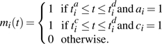Similarly, m′_i(t) is defined to be equal to 1 if a patient is present on the ward and uncolonized at time t, and 0 otherwise.

The augmented number of colonized patients on the ward at time t is then given by

Transmission and importation model

In this section, we describe a baseline transmission and importation model. Variants of this model are considered later. In the baseline model, it is assumed that colonized patients are equally infectious, but susceptibility to becoming colonized may vary with the study phase and patient characteristics. The probability of patient i (assumed to be initially uncolonized) becoming colonized in a short interval (t, t + Δt) is λ_i(t)y(t)Δt + o(Δt) for some transmission parameter λ_i(t).

It follows that the likelihood expression for the transmission model is

(1)

Here, t_i−^c represents the time immediately before t_i^c. In our implementation, event times are resolved at the level of days, so all events are assumed to occur only at the beginning of each day and t_i−^c is taken as t_i^c−1. The product of exponential terms in (equation 1 corresponds to the likelihood of transmission not occurring, and the second product term gives the likelihood of transmission events that did occur (refer, for example, to Becker (14) for a generalization of this formula). Note that this model does not allow inferences about who infected whom.

The importation probability, ν, represents the chance that patients already carry the strain when admitted to the ward. The likelihood of the set of admission colonization statuses, {a_i}, is therefore

(2)

This expression encodes the assumption that each patient admission is associated with an independent probability that the patient is already colonized when admitted.

The total likelihood of the transmission and importation model for a given realization of the augmented data is equal to the product of (equations 1 and (2.

A log-link function is used to express the effect of ward- and patient-level covariates on patient susceptibility:

where x₂,.(t) and x₃,.(t) are defined to be equal to 1 if t lies in study phase 2 and in study phase 3, respectively, and 0 otherwise (some models considered included additional covariates). The hazard ratios for colonization associated with these respective phases (due to a single colonized patient) are given by h₂ = exp(β₂) and h₃ = exp(β₃), and h₁ = exp(β₁) gives the baseline hazard rate when there is one other colonized patient on the ward.

Observation model

The observation model defines the probability of the observed data (the swab results), D, for a given set of values in the augmented data. Assuming there are no false positives, this probability is 0 if there exist i, j such that s_{i, j} = 1 and m_i (t_ij^s) = 0. Otherwise, it is given by

where ξ is the probability of correctly detecting the presence of the organism in a swab taken from a colonized patient (i.e., the sensitivity).

Prior model

Diffuse priors were used for all parameters: N(0, 1,000) for the β₁,β₂,… terms and Beta (1, 1) for ν and ξ.

Posterior inference

The joint posterior density of A, D, ν, ξ, and β₁,β₂,… is thus given as the product of the observation model, the transmission model, and the prior model:

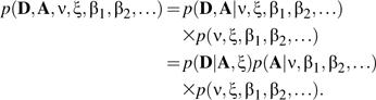(3)

The joint posterior density of ν, ξ, β₁,β₂,…, and A is then estimated numerically by using a Markov chain Monte Carlo sampling algorithm outlined below (full details are given in the supplementary technical appendix, which is posted on the Journal's website (http://aje.oupjournals.org/)). The unobserved times when patients acquire the organism (the latent event times, which are part of the augmented data) are included in the set of model unknowns. The number of acquisitions of the organism (and hence the number of unknowns) is itself an unknown, so the dimension of the model can change. A Markov chain Monte Carlo sampling algorithm with reversible jump extensions is therefore required to explore the joint posterior distribution of all model unknowns (the augmented data and the model parameters) (15).

Model variants

Here, we present results for seven variants of the basic model described above. In model I, λ_i(t) varies only by study phase, and swab sensitivity is assumed to be 100 percent. Patient readmissions are not explicitly accounted for, but, when patient screening swabs are positive in consecutive admission episodes, it is assumed that the patient was colonized on admission in the second episode. Since patients are assumed not to clear colonization during the course of a single admission, only those data up to the first positive swab for each episode are used when fitting model I.

Models II–VII remove the assumption of perfect swab sensitivity and use all the data. Model II is identical to model I, except that repeated admissions are not accounted for in any way. Models III–VII, in contrast, account for repeated admissions by allowing for the possible loss or acquisition of colonization between admissions. An exponentially distributed duration of colonization following discharge is assumed. Thus, the probability that a patient who is colonized when discharged is still colonized when readmitted t days later is exp(–ϕt), and the mean duration of colonization outside the ward is 1/ϕ days (again, since colonization is asymptomatic, it is assumed not to influence the probability of readmission). In all cases, a diffuse prior, Γ(0.001, 0.001), is used for ϕ. Five variants of this readmission model are considered (all with straightforward modifications to the likelihood):

1. In model III, patients who are not colonized at discharge are assumed to have the same phase-independent probability, ν, of being colonized on subsequent readmissions as patients with no previous documented admissions.

2. Model IV differs from model III only in incorporating patient-level covariates (age, gender, and protective isolation).

3. In model V, patients who are not colonized at discharge are assumed, on subsequent admission, to have phase-specific probabilities, (ν₁, ν₂, ν₃), of being colonized on admission. Patients with no previous documented admissions also have these phase-dependent probabilities of being colonized when admitted.

4. In model VI, patients without previous documented admissions have a phase-independent probability of being colonized on admission, ν. Patients who are not colonized at discharge are assumed to have a probability of being colonized on subsequent admission t days later, given by ν(t) = ν(1 – exp(–ϕt/(1 – ν))). This expression can be derived by assuming constant rates of acquisition and loss of colonization outside the ward and that ν represents the long-term equilibrium for the proportion outside the ward who are colonized.

5. In model VII, patients not colonized at discharge are treated as in model VI on subsequent admissions. Patients without previous documented admissions have phase-specific probabilities of being colonized on admission, as in model V.

Model comparison and assessment

Model comparison was based on a version of the deviance information criterion (DIC) (16). This criterion uses the deviance penalized by the effective number of parameters. A lower value indicates a better fit. Usually, it is calculated as DIC=+p_D. Here, p_D is given by −D(θ) (the posterior mean deviance minus the deviance at the posterior mean) and is interpreted as the effective number of model parameters. In this case, however, the augmented data are categorical, so there is no unique posterior mean. Instead, the effective number of parameters was estimated with p_D = var(D)/2 (17).

Two approaches were used to assess model fit. First, a cross-validatory approach was used to predict the results of the screening swabs for each patient in turn given the preceding day's augmented data (sampled from the posterior) for other patients. These predictions were made in two steps. First, predictions for the augmented data for each ward-day for each patient were obtained from a sequence of 1-day-ahead Monte Carlo samples from the transmission model (using one set of values for model parameters and augmented data sampled from their joint posterior). Second, the observation model was then used to obtain a sample of the predicted swab results (i.e., a swab from a patient who was colonized in the predicted augmented data was positive with probability ξ). One thousand such samples were taken and were used to compare predicted and observed “apparent acquisitions” on each study day (the first positive screening swab following one or more negative screening swabs for the same patient episode indicated an “apparent acquisition”).

The second approach assessed the ability of the different models to forecast the time evolution of the epidemic, conditioning on patient colonization statuses on the first day of the study and observed patient stays. Again, this approach required two steps: sampling from the transmission model, then sampling from the observational model. Each prediction sample again used one set of model parameters sampled from the posterior distribution, but otherwise these predictions made no use of individual swab results. In this case, observed and predicted swab results for each day of the study were compared.

Implementation

A Metropolis sampling algorithm was used to update the augmented data and model parameters (except ν and ξ, for which a Gibbs step was used) (18, 19). The algorithm was implemented in a C++ program (full details are given in the supplementary technical appendix) and was verified by using simulated data.

Convergence of the Markov chains was assessed by visual inspection and through the use of the single-chain diagnostics implemented in the Bayesian Output Analysis Program (BOA) package (20).

RESULTS

Reported results are based on at least 150,000 values sampled from the Markov chain, where a sample was taken at every 100th iteration (although chains up to four times this length were used to confirm convergence). Acceptance probabilities for proposed updates to the augmented data ranged from 28 percent (model VII) to 51 percent (model I). Samples from the posterior distribution indicated little correlation between parameter values, with the exception of β₁, which, in the unadjusted models, was negatively correlated with both β₂ and β₃ (figure 3).

FIGURE 3.

Pairwise plots of samples from the posterior distribution for swab sensitivity (ξ), probability of being admitted colonized (ν), rate of loss of colonization outside the ward (ϕ), and transmission rates for phases 1–3 (β₁, β₂, β₃). Plots below the diagonal show results from model III; those above show results from model IV (each point shows the value of two parameters from one sample from the posterior). Histograms on the diagonal show the marginal posterior distributions for model IV. Correlations between pairs of parameters are indicated in the top right of each subgraph.

The largest Monte Carlo error was usually associated with the phase 3 hazard ratio, h₃, for which the value of 0.005 obtained with model V and 150,000 values sampled was typical.

All models considered led to broadly similar conclusions about the effect of the interventions (tables 1 and 2): estimated values for h₂ provided good evidence that the phase 2 intervention substantially reduced patient-to-patient transmission (the contribution of each colonized patient to the transmission rate for each uncolonized patient falling by about half in phase 2). In contrast, all h₃ estimates were close to 1, with wide credible intervals, indicating that there was little evidence that the phase 3 transmission rate differed from that in phase 1, despite the educational intervention.

TABLE 1.

Parameter estimates: medians and 95% credible intervals for models I–IV^*

Parameter	Model
	I		II		III		IV
	Median	95% credible interval	Median	95% credible interval	Median	95% credible interval	Median	95% credible interval
Probability of being admitted colonized (ν)	0.21	0.16, 0.26	0.14	0.09, 0.19	0.09	0.06, 0.14	0.10	0.06, 0.15
Baseline transmission × 103(h1)	5.3	3.6, 7.4	7.6	5.1, 10.8	6.8	4.6, 9.8	3.9	1.4, 9.1
Phase 2 hazard ratio (h2)	0.50	0.26, 0.90	0.38	0.17, 0.75	0.39	0.18, 0.78	0.30	0.11, 0.64
Phase 3 hazard ratio (h3)	0.99	0.51, 1.82	1.08	0.53, 2.05	1.13	0.53, 2.22	0.90	0.37, 2.03
Swab sensitivity (ξ)			0.90	0.85, 0.94	0.89	0.85, 0.93	0.89	0.84, 0.93
Mean duration of carriage (days) (1/ϕ)					98.7	47.4, 218.8	97.4	45.8, 219.2
Protective isolation							1.8	0.8, 4.2
Male gender							1.8	0.9, 3.5
Age (second quartile)							0.9	0.4, 2.3
Age (third quartile)							0.8	0.3, 2.0
Age (fourth quartile)							1.6	0.6, 4.0
Δ DIC†	NA†		0	Baseline	−131		−113

^*Model I assumes perfect swab sensitivity, model II allows for imperfect swab sensitivity but no readmission, model III extends model II to allow for patient readmissions, and model IV extends model III to adjust for patient-level covariates. The parameters h₂ and h₃ (which are equal to exp(β₂) and exp(β₃)) represent the ratios of the hazards for a susceptible patient to acquire the organism in phases 2 and 3 compared with phase 1, given the same number of colonized patients. Values less than one indicate a decreased risk of transmission.

^†DIC, deviance information criterion; NA, not applicable.

TABLE 2.

Parameter estimates: medians and 95% credible intervals for models V–VII^*

Parameter	Model
	V		VI		VII
	Median	95% credible interval	Median	95% credible interval	Median	95% credible interval
Probability of being admitted colonized (all phases) (ν)			0.11	0.07, 0.17
Probability of being admitted colonized (phase 1) (ν1)	0.28	0.17, 0.41			0.25	0.15, 0.37
Probability of being admitted colonized (phase 2) (ν2)	0.03	0.01, 0.09			0.03	0.00, 0.08
Probability of being admitted colonized (phase 3) (ν3)	0.03	0.00, 0.11			0.03	0.00, 0.12
Baseline transmission × 103(h1)	6.1	3.9, 8.8	6.9	4.6, 9.7	6.5	4.3, 9.3
Phase 2 hazard ratio (h2)	0.54	0.25, 1.05	0.39	0.17, 0.78	0.50	0.25, 0.95
Phase 3 hazard ratio (h3)	1.33	0.62, 2.61	1.06	0.50, 2.08	1.21	0.57, 2.37
Swab sensitivity (ξ)	0.90	0.85, 0.94	0.89	0.85, 0.93	0.90	0.85, 0.93
Mean duration of carriage (days) (1/ϕ)	105.0	51.0, 236.7	117.5	56.2, 264.3	116.8	57.4, 259.1
Δ DIC†	−583		−170		−201

^*Models V, VI, and VII are identical to model III (refer to table 1) except in the following respects: for patients who are uncolonized at the end of a previous admission (or who have no previous admissions), model V allows the probability of being colonized on admission to depend on the study phase; model VI allows the probability of being colonized on admission for those who are not colonized at the end of a previous admission to depend on the time to readmission, as described in the text; and model VII combines aspects of models V and VI, with probabilities of being colonized on admission varying by study phase for those with no previous admissions and by time since discharge for those uncolonized at the end of their previous admission.

^†DIC, deviance information criterion.

Removing model I's arbitrary assumptions about the colonization status of readmitted patients and allowing for imperfect swab sensitivity led to a much lower estimated probability that patients were admitted colonized and to a much higher estimate of the baseline transmission parameter (model II). Models allowing for patient readmission (III–VII) all estimated a mean duration of carriage of vancomycin-resistant enterococci outside the ward of approximately 100 days (but with wide credible intervals) and gave similar estimates for swab sensitivity to model II (close to 90 percent). Comparison of deviance information criteria between models II through VII (model I uses different data and is not comparable) indicated that accounting for the readmission of patients in models II–VII substantially improved the model fit (lowered the deviance information criterion). There was no strong evidence that the potential confounders in model IV were associated with altered transmission, although there was weak evidence that male patients and those in the oldest quartile were at increased risk of acquiring vancomycin-resistant enterococci. Including patient-level covariates (model IV), however, gave a higher deviance information criterion than that for model III, indicating a worse fit. Patient-level covariates were therefore not included in the other models.

Model assessment using the cross-validatory method suggested that models I–IV all gave adequate fits to the data (figure 4, top). This visual impression was confirmed by a chi-squared test of goodness of fit, comparing the total observed and mean predicted numbers of apparent acquisitions by study phase. For example, with model III, the cross-validatory approach predicted the mean number of apparent acquisitions to be 20.7, 11.1, and 9.9 in phases 1, 2 and 3, respectively, compared with 21, 13, and 10 observed (χ² = 1.07, df = 2; p = 0.59).

FIGURE 4.

Model assessment using cross-validatory (top) and forecasting (bottom) approaches for models III (left) and V (right). The cross-validatory approach compares the number of observed apparent acquisition events (initial negative followed by positive swabs from the same patients) with corresponding posterior predictions for each patient, conditioning on the earlier swab results from other patients. The forecasting approach compares observed and predicted positive swabs taken on each day, conditioning only on the colonization status of patients on the first study day and on the admission and discharge dates for each patient. In all cases, 50-day moving averages are shown for data (solid line), median predicted values (dashed line), and 95% credible intervals for predictions (dotted lines).

In contrast, the forecasting approach found that these models consistently predicted more swabs positive for vancomycin-resistant enterococci than observed between days 275 and 375 (figure 4, bottom). This lack of fit was confirmed by a further chi-squared goodness-of-fit test comparing observed and predicted positive swabs by phase (χ² = 14.6, df = 2; p = 0.001). It was this discrepancy that led to consideration of the model variants V–VII. All these models had lower deviance information criterion values than model III, but the largest improvement in model fit was obtained when the probability of being admitted colonized (for those who were not previously discharged colonized) was allowed to vary by study phase (model V). Forecasts obtained by using this model showed a notable improvement between day 275 and day 375, with observed data falling within 95 percent forecast intervals, and adequate goodness of fit (χ² = 3.20, df = 2; p = 0.20). Nonetheless, even with the best model, there was still a tendency to overestimate the prevalence of vancomycin-resistant enterococci during this period.

DISCUSSION

The approach described here builds on methods developed for studying epidemics in the community (21–23) and a recent adaptation of these methods to hospital populations (24). This work extends these approaches to account for repeated admissions by explicitly modeling the loss of carriage following discharge. It also shows how these methods can be applied to the analysis of interrupted time-series studies without having to make arbitrary assumptions about transmission events and allowing for adjustment for potential confounders and estimation of important parameters, such as duration of carriage outside the ward and swab sensitivity.

In addition to the approach described by Forrester et al. (24), four other approaches to analyzing nosocomial infection data using stochastic transmission models have been described. The first used a Markov model to analyze repeated cross-sectional screening data (so it would not be suitable for the arbitrarily timed swab data used here) (25). The second used a hidden Markov model to analyze time series of infection counts rather than colonization data (3). A limitation of this approach is that infections occur much less frequently and the information content of such data is much lower. The third approach overcame some of these limitations of sparse data by using a Bayesian implementation of the hidden Markov model (26).

The fourth approach used surveillance data from arbitrarily timed swabs to fit a stochastic transmission model using a likelihood approach, making use of observed stays of individual patients (27). This approach is the closest of the four to the method described here, and it has one clear advantage: model fitting is much speedier. The augmented data framework adopted here, however, at the cost of being computationally much more demanding, offers greater flexibility, making it possible to account for important epidemiologic features such as repeated admissions and imperfect swab sensitivity.

Imperfect observation of highly dependent longitudinal data poses a number of problems, many of which we have addressed but some of which remain. Initial conditions present a special problem when states are not perfectly observed because, by definition, there are no earlier data, so the probability that patients already present at t = 0 were colonized on admission cannot be modeled in the manner used at subsequent time points. Here, the issue was sidestepped by assuming that patients initially on the ward were admitted at t = 0. This censoring may become even more important when patients are admitted multiple times. The two best-fitting models (V and VII) were those allowing phase-specific probabilities of colonization on admission. Both models estimated large reductions in this probability after phase 1, almost certainly because patients admitted in phase 1 who were not known to be previously colonized would have included many with unobserved prestudy admissions. Any vancomycin-resistant enterococci colonization during these earlier admissions would not have been detected, and such colonized patients would therefore contribute to the estimate of ν₁, the phase 1 importation probability. In contrast, patients admitted in phases 2 and 3 who were colonized during earlier stays on the ward during the study would be identified as previously colonized patients. These patients would therefore not contribute to the estimates of the importation probabilities ν₂ and ν₃, resulting in much lower estimates.

Recent models of methicillin-resistant Staphylococcus aureus transmission have allowed for a constant background rate of acquisition (in addition to importation and patient-to-patient transmission) to account for other sources of within-ward acquisitions (such as colonized relatives or staff) (24). These sources were not believed to be important in the current context and were not considered in the model.

All the models considered here assumed that patients, once colonized, remained so until discharge. While a more general model would allow for within-ward loss of colonization, it was found that, once colonized, patients invariably remained so until discharge. Repeated therapy with antianaerobic antibiotics, which appears to promote high-level carriage persistence, may be one reason rapid carriage clearance appeared to be unimportant (28). A further limitation of the current work is the absence of a washout period. However, by accounting for readmissions, the model was able to capture at least one source of carryover effects.

Understanding the effect of antibiotic use on the transmission and persistence of drug-resistant bacteria presents major difficulties for conventional approaches to data analysis: antibiotics may select for resistant strains both by increasing the risk of acquisition (by suppressing competing organisms) and by increasing transmission from treated colonized patients (by increasing levels of carriage). They may also alter the probability of detecting colonization (29). Extensions of methods such as those considered here have the potential to help overcome these obstacles and could play a major role in addressing key scientific questions in this field.

References

- 1.Becker NG, Britton N. Statistical studies of infectious disease incidence. J R Stat Soc Ser (B) 1999;61:287–307. [Google Scholar]
- 2.Cooper BS, Stone SP, Kibbler CC, et al. Isolation measures in the hospital management of methicillin resistant Staphylococcus aureus (MRSA): systematic review of the literature. BMJ. 2004;329:533. doi: 10.1136/bmj.329.7465.533. [DOI] [PMC free article] [PubMed] [Google Scholar]
- 3.Cooper B, Lipsitch M. The analysis of hospital infection data using hidden Markov models. Biostatistics. 2004;5:223–37. doi: 10.1093/biostatistics/5.2.223. [DOI] [PubMed] [Google Scholar]
- 4.Smith DL, Dushoff J, Perencevich EN, et al. Persistent colonization and the spread of antibiotic resistance in nosocomial pathogens: resistance is a regional problem. Proc Natl Acad Sci U S A. 2004;101:3709–14. doi: 10.1073/pnas.0400456101. [DOI] [PMC free article] [PubMed] [Google Scholar]
- 5.Cooper BS, Medley GF, Stone SP, et al. Methicillin-resistant Staphylococcus aureus in hospitals and the community: stealth dynamics and control catastrophes. Proc Natl Acad Sci U S A. 2004;101:10223–8. doi: 10.1073/pnas.0401324101. [DOI] [PMC free article] [PubMed] [Google Scholar]
- 6.Bootsma MC, Diekmann O, Bonten MJ. Controlling methicillin-resistant Staphylococcus aureus: quantifying the effects of interventions and rapid diagnostic testing. Proc Natl Acad Sci U S A. 2006;103:5620–5. doi: 10.1073/pnas.0510077103. [DOI] [PMC free article] [PubMed] [Google Scholar]
- 7.Robotham JV, Scarff CA, Jenkins DR, et al. Methicillin-resistant Staphylococcus aureus (MRSA) in hospitals and the community: model predictions based on the UK situation. J Hosp Infect. 2007;65(suppl 2):93–9. doi: 10.1016/S0195-6701(07)60023-1. [DOI] [PubMed] [Google Scholar]
- 8.Jernigan JA, Titus MG, Groschel DH, et al. Effectiveness of contact isolation during a hospital outbreak of methicillin-resistant Staphylococcus aureus. Am J Epidemiol. 1996;143:496–504. doi: 10.1093/oxfordjournals.aje.a008770. [DOI] [PubMed] [Google Scholar]
- 9.Williams R, Noble W, Jevons M, et al. Isolation for the control of staphylococcal infection in surgical wards. Br Med J. 1962;2:275–82. doi: 10.1136/bmj.2.5300.275. [DOI] [PMC free article] [PubMed] [Google Scholar]
- 10.Shooter R, Thom B, Dunkerley D, et al. Pre-operative segregation of patients in a surgical ward. Br Med J. 1963;2:1567–9. doi: 10.1136/bmj.2.5372.1567. [DOI] [PMC free article] [PubMed] [Google Scholar]
- 11.Lidwell O, Davies J, Payne R, et al. Nasal acquisition of Staphylococcus aureus in partly divided wards. J Hyg (Camb) 1971;69:113–23. doi: 10.1017/s002217240002132x. [DOI] [PMC free article] [PubMed] [Google Scholar]
- 12.Bradley S, Wilson A, Allen M, et al. The control of hyperendemic glycopeptide-resistant Enterococcus spp. on a haematology unit by controlling antibiotic usage. J Antimicrob Chemother. 1999;43:261–6. doi: 10.1093/jac/43.2.261. [DOI] [PubMed] [Google Scholar]
- 13.Bradley S, Kaufmann M, Happy C, et al. The epidemiology of glycopeptide-resistant enterococci on a haematology unit—analysis by pulsed-field gel electrophoresis. Epidemiol Infect. 2002;129:57–64. doi: 10.1017/s0950268802007033. [DOI] [PMC free article] [PubMed] [Google Scholar]
- 14.Becker N. London, United Kingdom: Chapman and Hall; 1989. Analysis of infectious disease data. [Google Scholar]
- 15.Green P. Reversible jump Markov chain Monte Carlo computation and Bayesian model determination. Biometrika. 1995;82:711–32. [Google Scholar]
- 16.Spiegelhalter D, Best N, Carlin B, et al. Bayesian measures of model complexity and fit. J R Stat Soc Ser (B) 2002;64:583–616. [Google Scholar]
- 17.Gelman A, Carlin J, Stern H, et al. Boca Raton, FL: Chapman and Hall; 2004. Bayesian data analysis. 2nd ed. [Google Scholar]
- 18.Gamerman D. London, United Kingdom: Chapman and Hall; 1997. Markov chain Monte Carlo: stochastic simulation for Bayesian inference. [Google Scholar]
- 19.Gilks W, Richardson S. Markov chain Monte Carlo in practice. In: Spiegelhalter D, editor. London, United Kingdom: Chapman and Hall/CRC; 1996. [Google Scholar]
- 20.Bayesian Smith B. Output Analysis program (boa), version 1.1.5. 2005. ( http://www.public-health.uiowa.edu/boa) [Google Scholar]
- 21.Gibson G, Renshaw E. Estimating parameters in stochastic compartmental models using Markov chain methods. IMA J Math Appl Med Biol. 1998;15:19–40. [Google Scholar]
- 22.O'Neill PD, Roberts GO. Bayesian inference for partially observed stochastic epidemics. J R Stat Soc Ser (A) 1999;162:121–9. [Google Scholar]
- 23.Auranen K, Arjas E, Leino T, et al. Transmission of pneumococcal carriage in families: a latent Markov process model for binary longitudinal data. J Am Stat Assoc. 2000;95:1044–53. [Google Scholar]
- 24.Forrester ML, Pettitt AN, Gibson GJ. Bayesian inference of hospital-acquired infectious diseases and control measures given imperfect surveillance data. Biostatistics. 2007;8:383–401. doi: 10.1093/biostatistics/kxl017. [DOI] [PubMed] [Google Scholar]
- 25.Pelupessy I, Bonten MJ, Diekmann O. How to assess the relative importance of different colonization routes of pathogens within hospital settings. Proc Natl Acad Sci U S A. 2002;99:5601–5. doi: 10.1073/pnas.082412899. [DOI] [PMC free article] [PubMed] [Google Scholar]
- 26.McBryde ES, Pettitt AN, Cooper BS, et al. Characterizing an outbreak of vancomycin-resistant enterococci using hidden Markov models. J R Soc Interface. 2007;4:745–54. doi: 10.1098/rsif.2007.0224. [DOI] [PMC free article] [PubMed] [Google Scholar]
- 27.Bootsma MC, Bonten MJ, Nijssen S, et al. An algorithm to estimate the importance of bacterial acquisition routes in hospital settings. Am J Epidemiol. 2007;166:841–51. doi: 10.1093/aje/kwm149. [DOI] [PubMed] [Google Scholar]
- 28.Donskey C, Hanrahan J, Hutton R, et al. Effect of parenteral antibiotic administration on persistence of vancomycin-resistant Enterococcus faecium in the mouse gastrointestinal tract. J Infect Dis. 1999;180:384–90. doi: 10.1086/314874. [DOI] [PubMed] [Google Scholar]
- 29.Harbarth S, Cosgrove S, Carmeli Y. Effects of antibiotics on nosocomial epidemiology of vancomycin-resistant enterococci. Antimicrob Agents Chemother. 2002;46:1619–28. doi: 10.1128/AAC.46.6.1619-1628.2002. [DOI] [PMC free article] [PubMed] [Google Scholar]
Associated Data
This section collects any data citations, data availability statements, or supplementary materials included in this article.