Bounds and Algorithms for Fast Exact Searches of Chemical Fingerprints in Linear and Sub-Linear Time

Abstract

Chemical fingerprint are used to represent chemical molecules by recording the presence or absence, or by counting the number of occurrences, of particular features or substructures, such as labeled paths in the 2D graph of bonds, of the corresponding molecule. These fingerprint vectors are used to search large databases of small molecules, currently containing millions of entries, using various similarity measures, such as the Tanimoto or Tversky's measures and their variants. Here we derive simple bounds on these similarity measures, and show how these bounds can be used to considerably reduce the subset of molecules that need to be searched. We consider both the case of single-molecule and multiple-molecule queries, as well as queries based on fixed similarity thresholds or aimed at retrieving the top K hits. We study the speedup as a function of query size and distribution, fingerprint length, similarity threshold, and database size |D| and derive analytical formula that are in excellent agreement with empirical values. The theoretical considerations and experiments show that this approach can provide linear speedups of one or more orders of magnitude in the case of searches with fixed threshold, and achieve sublinear speedups in the range of O(|D|^0.6) for the top K hits in current large databases. This pruning approach yields subsecond search times across the 5M compounds in the ChemDB database, without any loss of accuracy.

1 Introduction

One of the most fundamental tasks of chemoinformatics is the rapid search of large repositories of molecules. In a typical search, given a query consisting of a molecule or a family of molecules, one is interested in retrieving all the molecules contained in a large repository such as PubChem, ZINC,¹ or ChemDB,² that are similar to the query and satisfy the given constraints. To facilitate this process, in many chemoinformatics systems, molecules are represented by binary fingerprint vectors^3-7 (and references therein). It is these fingerprints and their similarity measures that are used to search these large repositories. While fingerprint representations yield efficient search algorithms, it is still important to keep search times to a minimum to allow interactive searches and to allow the search space to grow considerably beyond its current typical value of a few million molecules towards the estimated 10⁶⁰ size of the virtual space of small organic molecules.⁸ To further reduce search times, here we first derive bounds on all the standard similarity measures and then show how these bounds can be used to prune the search space and considerably speed up current searches, without any loss of accuracy.

2 Molecular Fingerprint Notation and Similarity Measures

2.1 Molecular Fingerprint Notation

Let $\mathcal{A}$ denote a molecule, and $\overrightarrow{A}$ = (A_i) the corresponding fingerprint vector, with 1 ≤ i ≤ N . The precise interpretation of the fingerprint components is irrelevant for our purpose. As in most chemoinformatics systems, one may consider that each component A_i is a bit associated with the presence or absence of a particular substructure (e.g. functional group, labeled path, labeled cycle, labeled tree) of atoms and bonds in the molecule. While many systems use binary fingerprints, it is also possible to use richer, integer-valued, fingerprints where the components A_i count the number of occurrences of the corresponding substructure. Here the length N of the fingerprints is not important–our considerations apply to full-length fingerprints (large values of N), compressed fingerprints (typically N = 512 or N = 1024), or variable-length fingerprints. For each fingerprint $\overrightarrow{A}$, we let A = Σ_i A_i. In the binary case, A is the total number of bits set to one. In the general case, A is the sum of all substructure counts. In the binary case, we also use $A\cup B$ (resp. $A\cap B$) to denote the total number of bits set to one in $\overrightarrow{A}$ OR $\overrightarrow{B}$ (resp. $\overrightarrow{A}$ AND $\overrightarrow{B}$).

While in current systems queries are often based on a single molecule, sometimes it is useful to use several related molecules in a query of the form $\stackrel{‒}{\mathcal{A}}$ = {${\mathcal{A}}_1,\dots {\mathcal{A}}_M$}, as in the example of Figure 1. In this notation, ${\mathcal{A}}_i$ represents the i-th molecule in the family, and M = $\mid \stackrel{‒}{\mathcal{A}}\mid$ represents the number molecules in the query. In this case, ${\overrightarrow{A}}_i$ = (A_ij) denotes the fingerprint vector associated with molecule ${\mathcal{A}}_i$, and A_i = Σ_j A_ij.

Figure 1.

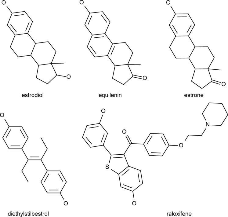
Examples of five Estrogen Receptor binding compounds that could be entered in a multiple-molecule query aimed at retrieving additional compounds in the same family.

2.2 Molecular Similarity Measures

The measure used to assess similarity between molecules, hence fingerprints, plays a fundamental role in chemical searches. Several similarity measures have been introduced for molecular fingerprints, two of the most common ones being the Tanimoto measure and its generalization, the Tversky measure, for binary fingerprints.^9,10 Both measures can be generalized to fingerprints based on counts using a MinMax operator,¹¹ as described below. Our derivations here are illustrated primarily with the Tanimoto and Tversky measures in the binary case, since these are the most widely used, but we treat also their extensions to the non-binary case. Moreover, the same ideas can be applied immediately to many other fingerprint similarity measures, as described in the Appendix.

The Tanimoto similarity measure between two binary fingerprints is defined by the ratio of the number of common bits set to one to the total number of bits set to one in the two fingerprints

$$S\left(A,B\right)=S(\overrightarrow{A},\overrightarrow{B})=(A\cap B)∕(A\cup B)$$ (1)

The Tanimoto coefficient is essentially a variation on the F measure of information retrieval.¹²

The Tversky measure with parameters α and β between two binary fingerprints is defined by

$$S_{\alpha \beta }(\overrightarrow{A},\overrightarrow{B})=\frac{A\cap B}{\alpha A+\beta B+(1-\alpha -\beta )(A\cap B)}$$ (2)

with 0 ≤ α and 0 ≤ β. When α = β = 1 it reduces to the Tanimoto measure. In the non-symmetric case (α ≠ β), α and β are used for biasing the search towards superstructures or substructure of the query molecule $\mathcal{A}$. A large relative value of α will bias the search toward superstructures of $\mathcal{A}$, whereas a large relative value of β will bias the search towards substructures of $\mathcal{A}$.

For non-binary fingerprints associated with actual counts, the MinMax measure^11,13 is given by

$$S^C(\overrightarrow{A},\overrightarrow{B})=\frac{\sum _i\min (A_i,B_i)}{\sum _i\max (A_i,B_i)}$$ (3)

The MinMax measure reduces to the Tanimoto measure in the case of binary fingerprints.

Finally, for non-binary fingerprints, we can also generalize the Tversky measure to get the MinMax Tversky measure

$$S_{\alpha \beta }^C(\overrightarrow{A},\overrightarrow{B})=\frac{\sum _i\min (A_i,B_i)}{\alpha \sum _i{A}_i+\beta \sum _i{B}_i+(1-\alpha -\beta )\sum _i\min (A_i,B_i)}$$ (4)

which reduces to the Tversky measure in the case of binary fingerprints, and to the MinMax measure in the symmetric case with α = β = 1.

3 Bounds on Similarity for Single-Molecule Query

Let $\overrightarrow{A}$ be the query fingerprint. We can calculate efficient upper bounds for all the similarity measures described in the literature (see also Appendix). The upper bound for the Tanimoto similarity can be computed by writing the similarity as $S(\overrightarrow{A},\overrightarrow{B})=(A\cap B)∕(A+B-A\cap B)$ and noticing that the derivative of f(x) = x/(A + B − x) with respect to x is positive. Thus the derivative of the Tanimoto similarity is positive with respect to ($A\cap B$) and an upper bound can be derived by setting the number of bits in common ($A\cap B$) to its maximum possible value: min (A, B). In other words, for fixed $\overrightarrow{A}$ and $\overrightarrow{B}$,

$$S(\overrightarrow{A},\overrightarrow{B})\le T(A,B)=\frac{\min (A,B)}{A+B-\min (A,B)}=\frac{\min (A,B)}{\max (A,B)}$$ (5)

Here and everywhere else, S is used to denote the similarity measure and T the bound.

Using similar reasoning, we can derive a more general bound on the Tversky similarity in the form

$$S_{\alpha \beta }(\overrightarrow{A},\overrightarrow{B})\le T_{\alpha \beta }(A,B)=\frac{\min (A,B)}{\alpha A+\beta B+(1-\alpha -\beta )\min (A,B)}$$ (6)

In the case of the MinMax similarity for non-binary vectors, we have

$$S^C(\overrightarrow{A},\overrightarrow{B})\le T^C(A,B)=\frac{\min (A,B)}{A+B-\min (A,B)}=\frac{\min (A,B)}{\max (A,B)}$$ (7)

This bound uses the fact that Σ_i min(A_i, B_i). ≤ min (A, B) and Σ_i max(A_i, B_i) = A+B−Σ_i min(A_i, B_i).

It is also a special case of the bound on the MinMax Tverky similarity with α = β = 1, as given below.

In the case of the MinMax Tversky similarity for non-binary vectors, by combining the arguments above, we get the bound

$$S_{\alpha \beta }^C(\overrightarrow{A},\overrightarrow{B})\le T_{\alpha \beta }^C(A,B)=\frac{\min (A,B)}{\alpha A+\beta B+(1-\alpha -\beta )\min (A,B)}$$ (8)

It is worth noting that all the general bounds we have derived are optimal in the sense that one can construct examples where these bounds are actually achieved.

4 Bounds on Similarity for Multiple-Molecule Query

When the query is a family of molecules $\stackrel{‒}{\mathcal{A}}=\{{\mathcal{A}}_1,\dots {\mathcal{A}}_M\}$. there are basic ways of defining a similarity measure $S(\stackrel{‒}{\mathcal{A}},\mathcal{B})=S({\mathcal{A}}_1,\dots ,{\mathcal{A}}_M,\mathcal{B})=S({\overrightarrow{A}}_1,\dots ,{\overrightarrow{A}}_M,\overrightarrow{B})$ between the query family and each molecule B in the database: (1) by aggregating the individual pairwise similarity measures $S({\mathcal{A}}_i,\mathcal{B})=S({\overrightarrow{A}}_i,\overrightarrow{B})$; and (2) by aggregating the fingerprints ${\overrightarrow{A}}_i$ into a profile fingerprint $\overrightarrow{P}$, and then using a similarity measure of the form $S(\overrightarrow{P},\overrightarrow{B})$. With obvious adjustments, the ideas presented here can easily be extended to “family-family” (or “profile-profile”) comparisons of the form $S(\stackrel{‒}{\mathcal{A}},\stackrel{‒}{\mathcal{B}})=S({\mathcal{A}}_1,\dots ,{\mathcal{A}}_M,{\mathcal{B}}_1,\dots ,{\mathcal{B}}_Q)$ between two families $\stackrel{‒}{\mathcal{A}}$ and $\stackrel{‒}{\mathcal{B}}$ of molecules, where $\stackrel{‒}{\mathcal{B}}=\{{\mathcal{B}}_1,\dots ,{\mathcal{B}}_Q\}$.

4.1 Bounds on Aggregated Similarity for Multiple-Molecule Query

In the first class of approaches, the similarity $S(\stackrel{‒}{\mathcal{A}},\mathcal{B})$ is defined in terms of the individual similarities S(A_i, B), for instance by taking their weighted average, maximum, or minimum. In each one of these cases, bounds can easily be derived using the bounds obtained in Section 3. In the case of a weighted average with non-negative weights w₁ ...w_M ,we have

$$S({\mathcal{A}}_1,\dots ,{\mathcal{A}}_M,\mathcal{B})=\sum _i{w}_{i}S({\overrightarrow{A}}_i,\overrightarrow{B})\le \sum _i{w}_{i}T(A_i,B)$$ (9)

where S can be any of the similarities defined above and T the corresponding bound. Likewise, in the case where the family similarity is defined by the minimum pairwise similarity, we have

$$S({\mathcal{A}}_1,\dots ,{\mathcal{A}}_M,\mathcal{B})=\underset{i}{\min }S({\overrightarrow{A}}_i,\overrightarrow{B})\le \underset{i}{\min }T(A_i,B)$$ (10)

and for the maximum

$$S({\mathcal{A}}_1,\dots ,{\mathcal{A}}_M,\mathcal{B})=\underset{i}{\max }S({\overrightarrow{A}}_i,\overrightarrow{B})\le \underset{i}{\max }T(A_i,B)$$ (11)

Within the first class of approaches, it is also possible to consider measures that are obtained by combining the results of elementary pairwise comparisons between the molecules (e.g. intersections, unions) rather than the similarity measures themselves. In particular, one can derive a series of measures by simply aggregating the numerators and the denominators of the previous four similarity measures of Section 2. For instance, in the case of the binary Tversky measure, we can define an aggregate similarity measure

$$S_{\overrightarrow{\alpha }\overrightarrow{\beta }\overrightarrow{w}}({\mathcal{A}}_1,\dots ,{\mathcal{A}}_M,\mathcal{B})=\frac{\sum _i{w}_i(A_i\cap B)}{\sum _i{w}_i[{\alpha }_i{A}_i+{\beta }_{i}B+(1-{\alpha }_i-{\beta }_i)(A_i\cap B)]}$$ (12)

Note that each molecule ${\mathcal{A}}_i$ comes with two sets of parameters: a weight w_i which measures its importance among the family, and Tversky's parameters α_i and β_i which can be used to bias the search towards substructures or superstructures of ${\mathcal{A}}_i$. A special case of this particular measure is used in Xue et al. 2004.⁷

We can derive bounds on this measure by noticing again that the similarity has a positive derivative with respect to each term $A_i\cap B$ and using the inequality $A_i\cap B\le {\min }_i(A_i,B)$. This yields

$$S_{\overrightarrow{\alpha }\overrightarrow{\beta }\overrightarrow{w}}({\mathcal{A}}_1,\dots ,{\mathcal{A}}_M,\mathcal{B})\le T_{\overrightarrow{\alpha }\overrightarrow{\beta }\overrightarrow{w}}(A_1,\dots ,A_M,B)=\frac{\sum _i{w}_i\min (A_i,B)}{\sum _i{w}_i[{\alpha }_i{A}_i+{\beta }_i{B}_i+(1-{\alpha }_i-{\beta }_i)\min (A_i,B)]}$$ (13)

Likewise, a weighted MinMax measure can be written as

$$S_{\overrightarrow{w}}^C({\mathcal{A}}_1,\dots ,{\mathcal{A}}_M,\mathcal{B})=\frac{\sum _i{w}_i\sum _j\min (A_{ij},B_j)}{\sum _i{w}_i\sum _j\max (A_{i,j},B_j)}$$ (14)

Here A_ij denotes the j-th component of the fingerprint ${\overrightarrow{A}}_i$.

With even greater generality, we can consider a weighted MinMax Tversky similarity of the form

$$S_{\overrightarrow{\alpha }\overrightarrow{\beta }\overrightarrow{w}}^C({\mathcal{A}}_1,\dots ,{\mathcal{A}}_M,\mathcal{B})=\frac{\sum _i{w}_i\sum _j\min (A_{ij},B_j)}{\sum _i{w}_i[{\alpha }_i{A}_i+{\beta }_{i}B+\sum _j(1-{\alpha }_i-{\beta }_i)\min (A_{ij},B_j)]}$$ (15)

with the generalized bounds

$$S_{\overrightarrow{\alpha }\overrightarrow{\beta }\overrightarrow{w}}^C({\mathcal{A}}_1,\dots ,{\mathcal{A}}_M,\mathcal{B})\le T_{\overrightarrow{\alpha }\overrightarrow{\beta }\overrightarrow{w}}^C(A_1,\dots ,A_M,B)=\frac{\sum _i{w}_i\min (A_i,B)}{\sum _i{w}_i[{\alpha }_i{A}_i+{\beta }_{i}B+(1-{\alpha }_i-{\beta }_i)\min (A_i,B)]}$$ (16)

which can again be shown using somer algebra and noticing that the derivative of Equation 15 is positive with respect to Σ_i min(A_ij B_j) and that Σ_i min(A_ij B_j) ≤ min(A_i, B).

4.2 Bounds on Profile Similarity for Multiple-Molecule Query

A second possible class of approaches to multiple-molecule queries is to build a fingerprint profile $\overrightarrow{P}\left(\stackrel{‒}{\mathcal{A}}\right)=\overrightarrow{P}=\left(P_i\right)$ to represent the family $\stackrel{‒}{\mathcal{A}}$ and then measure similarity between the profile vector and the fingerprint vectors of the molecules to be searched. A fingerprint profile summarizes the information in a set of fingerprints, very much like a sequence profile or a position specific scoring matrix (PSSM) summarizes the information in a set of aligned sequences in bioinformatics. Fingerprint profiles can in turn be subdivided into linear and non-linear profiles.

A linear fingerprint profile stores for each component the frequency that the corresponding bit is set to one in the family of fingerprints. If a given bit position is set to one in half of the fingerprints in the family, then the corresponding component in the profile is set to 0.5. If the fingerprint consists of integer counts rather than bits, then the profile consists of average counts. In addition, different weights can also be assigned to each molecule or fingerprint in the family. In this more general case of linear profiles, Σ_i w_iA_ij. For proper scaling, it is desirable to use a convex combination with w_i ≤ 0 and Σ_i w_i = 1. Throughout this section, i =1,...M runs over the molecules in the family, and j =1,...N runs over the fingerprint components.

The similarity between the profile $\overrightarrow{P}\left(\stackrel{‒}{\mathcal{A}}\right)$ and a fingerprint $\overrightarrow{B}$ can be measured using the MinMax measure

$$S^C({\overrightarrow{P}}^w,\overrightarrow{B})=\frac{\sum _j\min (P_j^w,B_j)}{\sum _j\max (P_j^w,B_j)}$$ (17)

or the generalized MinMax Tversky measure

$$S_{\alpha \beta }^C({\overrightarrow{P}}^w,\overrightarrow{B})=\frac{\sum _j\min (P_j^w,B_j)}{\alpha \sum _j{P}_j^w+\beta \sum _j{B}_j+(1-\alpha -\beta )\sum _j\min (P_j^w,B_j)}$$ (18)

Letting A⁺ = P^w = Σ_j P^w_j = Σ_j Σ_i w_iA_ij, we can use the bounds on these measures to derive the bound

$$S^C({\overrightarrow{P}}^w,\overrightarrow{B})\le T^C(P^w,B)=\frac{\min (A^{+},B)}{A^{+}+B-\min (A^{+},B)}$$ (19)

and its more general version

$$S_{\alpha \beta }^C({\overrightarrow{P}}^w,\overrightarrow{B})\le T_{\alpha \beta }^C(P^w,B)=\frac{\min (A^{+},B)}{\alpha A^{+}+\beta B+(1-\alpha -\beta )\min (A^{+},B)}$$ (20)

In the case of a convex combination (Σ_i w_i = 1), we can derive an even better bound in the form

$$S_{\alpha \beta }^C({\overrightarrow{P}}^w,\overrightarrow{B})\le T_{\alpha \beta w}^C(A_1,\dots ,A_M,B)=\frac{\sum _i{w}_i\min (A_i,B)}{\sum _i{w}_i[\alpha A_i+\beta B_i+(1-\alpha -\beta )\min (A_i,B)]}$$ (21)

In other words, $S_{\alpha \beta }^C({\overrightarrow{P}}^w,\overrightarrow{B})\le T_{\alpha \beta w}^C(A_1,\dots ,A_M,B)\le T_{\alpha \beta }^C(P^w,B)$.

If the A_i's are binary and the combination is convex, then we have the identity ${\sum }_j\min (P_j^w,B_j)={\sum }_i{w}_i(A_i\cap B)$. Therefore, in the binary case with convex linear combination, we have the identities

$$S^C({\overrightarrow{P}}^w,\overrightarrow{B})=\frac{\sum _j\min (P_j^w,B_j)}{\sum _j\max (P_j^w,B_j)}=\frac{\sum _i{w}_i(A_i\cap B)}{\sum _i{w}_i[A_i+B-(A_i\cap B)]}$$ (22)

and

$$\begin{array}{cc}\hfill S_{\alpha \beta }^C({\overrightarrow{P}}^w,\overrightarrow{B})& =\frac{\sum _j\min (P_j^w,B_j)}{\sum _j\alpha P_j^w+\beta B_j+(1-\alpha -\beta )\sum _j\min (P_j^w,B_j)}\hfill \\ \hfill & =\frac{\sum _i{w}_i(A_i\cap B)}{\sum _i{w}_i[\alpha A_i+\beta B+(1-\alpha -\beta )(A_i\cap B)]}\hfill \end{array}$$ (23)

Thus, in the binary case, the MinMax and Tversky measures applied to the profile vectors ${\overrightarrow{P}}^w$ and $\overrightarrow{B}$ are equivalent to summing the numerators and denominators of the individual Tanimoto and Tversky measures between the A_i's and B (Equation 12), and thus the corresponding bound (Equation 13) can be applied. Note that, in the binary case, since the second family of approaches (profile) is a special case of the first family of approaches (aggregation), for bound purposes it is not necessary to compute the actual profile vector ${\overrightarrow{P}}^w$. This is not true in the non-binary case, or in the case of non-linear profiles described below.

To build non-linear profiles, a non-linear transformation is applied to the frequency counts in each column in order to derive a profile vector. In the case of consensus fingerprints,^6,15-17 for instance, the profile vector contains a one at a given position if and only if all the fingerprint vectors of the molecules in the query family also contain a one in that position. This can be generalized to modal fingerprints with threshold t,^16,17 by setting a bit to one in the profile vector if and only if the proportion of molecules in the query family that have a one at the corresponding position is greater or equal to t. Consensus profiles correspond to modal profiles with t = 1. Even more generally, a non-linear function such as a logistic function can be used to map frequencies to profile components. In the case of non-linear profiles, all the similarity bounds can still be used with the profile vector. The only difference with the linear case is that the bound in the non-linear case may not be easily expressed in terms of the bounds derived from the individual molecules in the query family.

5 Data

Before we show how the bounds can be used to speedup searches in large databases of compounds, we describe the data used in the experiments. All the data is extracted from the ChemDB database,² which currently contains on the order of 5M unique compounds. In the experiments, we use fingerprints associated with labeled paths of length up to 8 (i.e. 9 atoms and 8 bonds). In this case, the total number of observed labeled paths is N_* = 152,087. Compression is done using a simple modulo operator. Most results are reported for fingerprints of length N = 512. However we have tested all values N = 2ⁿ, with 5 ≤ n ≤ 10 and report the corresponding results when the dependence on fingerprint length is relevant. Robust results are obtained by increasing the path length or varying N_*, or N . All fingerprints are computed using an in-house program written in Python.

For experiments that require computing pairwise similarities between all molecules, we use a random data set of 50,000 molecules extracted from the ChemDB, corresponding approximately to 1.25 × 10⁹ pairwise similarity measurements. Varying the random sample does not affect these results in any significant way.

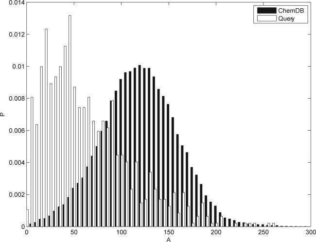
Figure 2 reports the distribution of A across the entire ChemDB database, together with the distribution of A over the queries received by ChemDB over the Web during a four-month period (02/06 to 06/06) The distribution of A across the entire database is well approximated by a Gaussian distribution with mean 119.53 and standard deviation 40.07. In contrast, the mean and standard deviation of the actual queries are 64.09 and 45.88 respectively.

Figure 2.

Empirical distributions of A = Σ_i A_i over the entire ChemDB, and over the set of ChemDB queries received over the Web during a period of four consecutive months, using fingerprints of length N = 512. The distribution of A across the entire database is well modeled using a Gaussian distribution with mean 119.53 and standard deviation 40.07. In contrast, the mean and standard deviation of the received queries are 64.09 and 45.88 respectively.

For some experiments we use the Stahl and Rarey¹⁴ datasets which consist of six groups of diverse molecules with similar activity. The molecules of each group are known to interact with the same protein. These datasets consists of 128 chemicals which interact with Cox-2, 55 which interact with Estrogen Receptor, 43 which interact with Gelatinase-A, 17 which interact with Neuraminidase, 25 which interact with p38-MAP Kinase, and 67 which interact with Thrombin. All datasets are available upon request.

6 Results: Fast Search Algorithms

6.1 Fast Search for Single-Molecule Query

We can now show how the bounds derived in the previous sections can be used to accelerate searches. For a given query and similarity threshold, we only need to sift through a small subset of molecules: those that satisfy the corresponding bound. More precisely, for any similarity measure, if we are interested in retrieving only molecules that have similarity to the query $\mathcal{A}$ above a given threshold t (0 ≤ t ≤ 1), then we can discard all the molecules $\mathcal{B}$ which satisfy T(A, B) ≤ t. This can drastically reduce the number of moleculeswhich must be examined, thereby improving speed without affecting accuracy at all.

For illustration purposes, consider first the simple case of binary fingerprints with Tanimoto similarity measure. For a query fingerprint of size A, Equation 5 shows that if B ≤ A then T(A, B) = B/A is linear in B. If B ≥ A, then T(A, B) = A/B and decays like 1/B (Figure 3). Thus all molecules with (B/A) < t can be discarded. Likewise, all molecules with (A/B) < t can be discarded. Thus the search can be restricted to molecules with B satisfying

$$At\le B\le \frac{A}{t}$$ (24)

Figure 3.

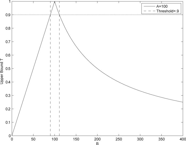
Pruning the search space. The binary fingerprint of the query molecule satisfies A = 100. As a function of B, the Tanimoto similarity measure $S(\overrightarrow{A},\overrightarrow{B})$ is upper bounded by the curve T(A, B). If the similarity threshold is set at 0.9, only molecules with B in a very small interval around 100 need to be searched. All other molecules have similarity scores that are below the threshold.

Likewise, for the Tversky similarity measure applied to binary fingerprints, we can discard all molecules with fingerprint vector $\overrightarrow{B}$ satisfying T_αβ(A, B) < t. Rearranging Equation 6, this shows that only molecules with fingerprint vector $\overrightarrow{B}$ satisfying

$$\frac{At\alpha }{1-t+t\alpha }\le B\le \frac{A(1-t+t\beta )}{t\beta }$$ (25)

need to be included in the search. Needless to say, the B values need to be computed only once for each molecule and then stored in the database. Therefore these bounds and the corresponding search restrictions can be implemented very efficiently. Similar considerations hold for all the other similarity measures (see also Appendix).

6.2 Fast Search for Multiple-Molecule Query

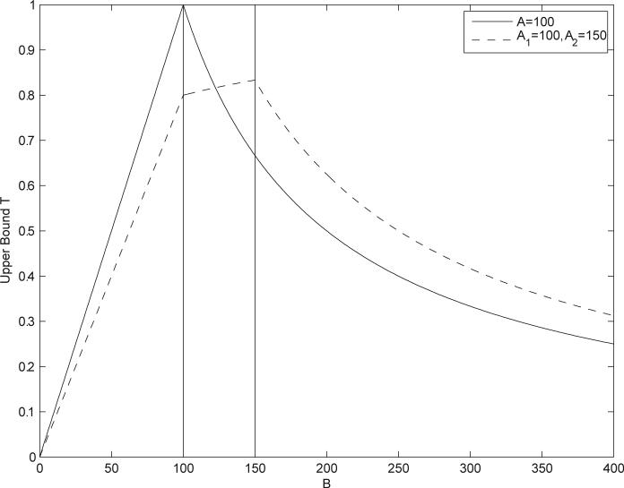
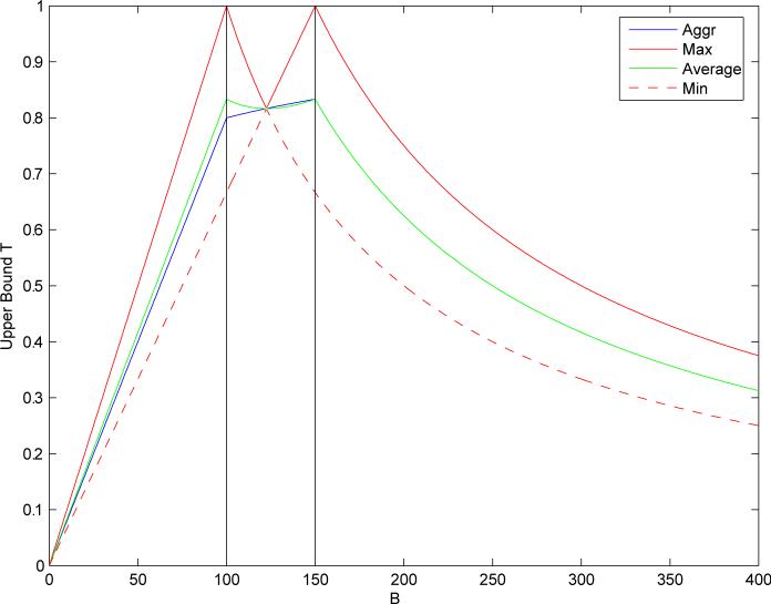
The same approach can be used for multiple-molecule queries. Figure 4, for instance, shows two curves corresponding to the bounds T on the Tanimoto measure, with a single-molecule query satisfying A = 100, as well as a two-molecule query with the two molecules satisfying A₁ = 100 and A₂ = 150. Figure 5 displays the bounds on different aggregate measures for the same two query molecules. By the same argument used in the case of single-molecule queries, at any given threshold we can draw a corresponding horizontal line and restrict the search to only those values of B for which the upper bound exceeds the line. For instance, in Figure 4 with a query consisting of two molecules satisfying A₁ = 100 and A₂ = 150 and a similarity threshold t = 0.85, we see that no molecule in the database can satisfy such conditions and therefore the result ought to be set to “empty” immediately.

Figure 4.

Bounds T on the Tanimoto measure as a function of the size B of the binary fingerprint of a molecule in the database. Solid curve corresponds to a single-molecule query with A = 100. Dashed curve corresponds to a two-molecule query with the two molecules satisfying A = 100 and A = 150, using the similarity measure in Equation 12, with α_i = β_i = 1 and w_i = 0.5 (also equivalent in this binary case to Equation 17).

Figure 5.

Bounds T on similarity measures as a function of the size B of the binary fingerprint of a molecule in the database. Two-molecule query with A₁ = 100 and A₂ = 150. Each curve corresponds to a different similarity measure. Average (green) is the average Tanimoto similarity across the two molecules in the query. Min (red dashed) [resp. Max (red)] is the minimum (resp. maximum) of the Tanimoto similarities. Aggregate (blue) is the aggregation of the individual Tanimoto similarity measures (Equation 12 with α_i = β_i = 1 and w_i = 0.5 for all i).

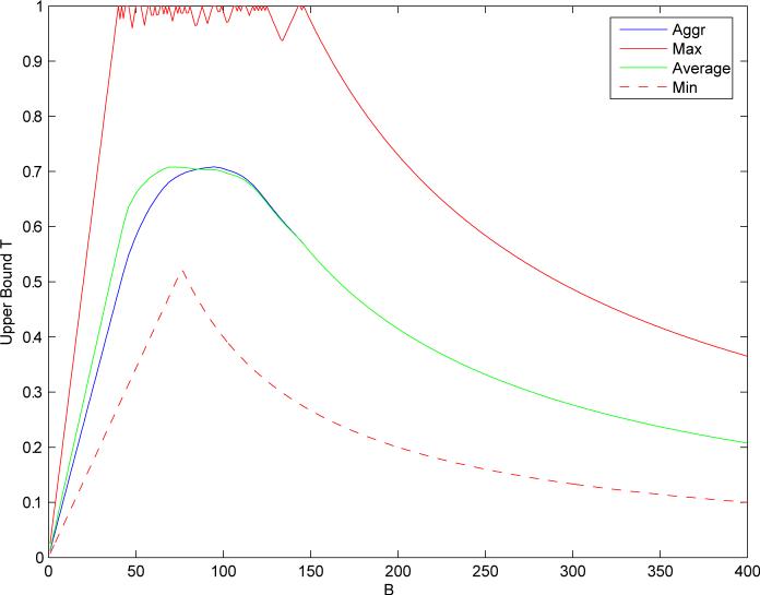
A more comprehensive and specific example is given in Figure 6 where the query molecules consist of a set of 55 Estrogen Receptor binding compounds,¹⁴ five of which are depicted in Figure 1.

Figure 6.

Bounds on similarity measure. Query consists of 55 Estrogen Receptor binding molecules against the same random sample of 50,000 molecules extracted from the ChemDB database. Molecules are represented by binary compressed fingerprints of length 512. Each curve corresponds to the bound for a different similarity measure. Average (green) is for the average Tanimoto similarity across the 55 molecules in the query. Min (red dashed) [resp. Max (red)] is for the minimum (resp. maximum) of the Tanimoto similarities. Profile (blue) is for the aggregation of the 55 individual Tanimoto similarity measures (Equation 12 with α_i = β_i = 1 and w_i = 1/55 for all i).

6.3 Top K Hits

Most often, however, one does not pre-specify a similarity threshold. Rather, as in most search engines and information retrieval systems, one is interested in finding the list of the most relevant hits. The methods described above can easily be adapted to the more realistic case where one is interested in retrieving the top K hits, without setting any arbitrary threshold. For this, we note that for single molecule queries the upper bound is unimodal. Thus we can search for the top K hits by starting from the maximum (where A=B), and exploring discrete possible values of B right and left of the maximum. More precisely, for binary fingerprints, we first index the molecules in the database by their fingerprint bit count to enable efficient referencing of a particular bit count bin. Next, with respect to a particular query, we calculate the bound on the similarity for every bit count in the database. Then we sort these bit counts by their associated bound and iterate over the molecules in the database, in order of decreasing bound. As we iterate, we calculate the similarity between the query and the database molecule and use a heap to efficiently track the top hits. The algorithm terminates when the lowest similarity value in the heap is greater than the bound associated with the current database bin. The algorithm is given below in simple pseudo-code form (Algorithm 1).

Algorithm 1	Top K Search
Require:	database of fingerprints $\overrightarrow{B}$ binned by bit count Bs
Ensure:	hits contains top K hits which satisfy Similarity($\overrightarrow{A},\overrightarrow{B}$) > T
1:	hits ← MinHeap()
2:	bounds ← List()
3:	for all B in database do //iterate over bins
4:	tuple ← Tuple(Bound(A,B),B)
5:	ListAppend(bounds, tuple)
6:	end for
7:	Quicksort(bounds) //NOTE: the length of bounds is constant
8:	for all bound, B in bounds do //iterate in order of decreasing bound
9:	if bound < T then
10:	break //threshold stopping condition
11:	end if
12:	if K ≤ HeapSize(hits) and bound <MinSimilarity(hits) then
13:	break //top-K stopping condition
14:	end if
15:	for all $\overrightarrow{B}$ in database[B] do
16:	S=Similarity($\overrightarrow{A},\overrightarrow{B}$)
17:	tuple ← Tuple(S,$\overrightarrow{B}$)
18:	if S ≤ T then
19:	continue //ignore this $\overrightarrow{B}$ and continue to next
20:	else if Length(hits)< K then
21:	HeapPush(hits, tuple)
22:	else if S > MinSimilarity(hits) then
23:	HeapPopMin(hits)
24:	HeapPush(hits,tuple)
25:	end if
26:	end for
27:	end for
28:	return hits

This algorithm is equally valid in the case of multiple-molecule queries. Even though the bounds for multiple-molecule queries can have multiple maxima (e.g. Figures 5 and 6), the bins are sorted in decreasing order of their bounds. Thus bounds with either single or multiple maxima are handled uniformly.

7 Results: Speedup

If f is the fraction of the database discarded by using the bounds, 1 — f is the fraction of the database to be searched and 1/(1 — f) is the speedup factor. The exact fraction of the database to be discarded from a given search and hence the speedup factor depends on many variables, primarily the query molecule(s), the similarity measure, and the similarity threshold t. In this section, we study f as a function of these variables, both empirically and analytically. When necessary, examples and details are given using the Tanimoto similarity measure, but extensions to other similarity measures should be obvious.

Theoretically, and in the experiments to be described, f alone provides a good assessment of the speedup because the overhead associated with the bounds is neglible. Evaluating the bounds takes at most O(N ) steps, where N is the fingerprint length. Sorting the bins by their associated bounds takes at most O(N log N ) steps. In practice, these overhead values are entirely negligible because N is quite small, in comparison with the size |D| of the database.

Using continuous notation, we let g_D(A) be the continuous density approximation to the values of A across the database D. When necessary, we use g_Q to denote the density over the queries, which can be different from g_D (Figure 2). The density g_D is well approximated using a Gaussian distribution with mean μ and standard deviation σ. These parameters in turn can depend on fingerprint length.

7.1 Speedup for Single-Molecule Query as a Function of Threshold and A

For a single-molecule query $\mathcal{A}$ and a threshold t, the bounds we have derived show that we need to search at most all the molecules satisfying x₀ ≤ B ≤ x₁, where the values of x₀ and x₁ depend on the value of A for the query molecule and on the similarity measure. Thus the fraction 1 — f of database to be searched satisfies

$$1-f\left(A\right)={\int }_{x_0}^{x_1}{g}_D\left(B\right)dB=G_D\left(x_1\right)-G_D\left(x_0\right)$$ (26)

where G_D is the corresponding distribution function. With Tanimoto similarity, for instance, combining Equations 24 and 26 with a Gaussian approximation yields

$$1-f\left(A\right)={\int }_{At}^{A∕t}{g}_D\left(B\right)dB=F\left(\frac{\frac{A}{t}-\mu }{\sigma }\right)-F\left(\frac{At-\mu }{\sigma }\right)$$ (27)

where F is the distribution function of the normalized standard Gaussian distribution. This expression can of course be computed numerically. When t is very close to 1, we can use the approximation

$$1-f\left(A\right)\approx \frac{A(1-t^2)}{t\sigma }\frac{1}{\sqrt{2\pi }}{e}^{-{(A-\mu )}^2∕2{\sigma }^2}\approx (1-t)\frac{2A}{\sqrt{2\pi \sigma }}{e}^{-{(A-\mu )}^2∕2{\sigma }^2}$$ (28)

so the speedup factor scales at least like C/(1 — t)when t is close to 1.

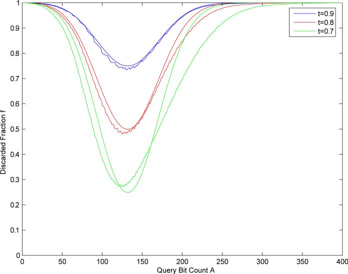
Figure 7 provides contour plots showing the fraction of the database f(A) to be excluded from a given search for the Tanimoto measure applied to compressed binary fingerprints of size 512, as a function of the query fingerprint size A, and for different threshold values: t = 0.7, t = 0.8, and t = 0.9. The fundamental result is that this fraction is very significant, and varies roughly from 30% to 100%, yielding searches that are faster by one or more orders of magnitude. In the worst case scenario, corresponding to A ≈ 120 for N = 512 or A_* ≈ 139 in the uncompressed fingerprint, the fraction varies from about 30% at t = 0.7 to about 75% at t = 0.9. In more favorable scenarios where A tends to be small or large, then the fraction is even larger. Note that for a fixed threshold the speedup factor is constant as a function of database size. As can be seen, the empirical curves agree very well with the theoretical approximation derived in Equation 28. Figure 8 provides a more complete picture of f as a function of A and t.

Figure 7.

Curves representing the fraction f of molecules discarded from a given search as a function of the size A of the binary query fingerprint, and the threshold t on the Tanimoto similarity. Blue corresponds to t = 0.9, red to t = 0.8, and green to t = 0.7. Results computed using a random sample of 50,000 molecules from the ChemDB database, using binary compressed fingerprint of length 512. The rough lines are the empirical curves. The smooth lines in this plot are the predictions provided by Equation 28.

Figure 8.

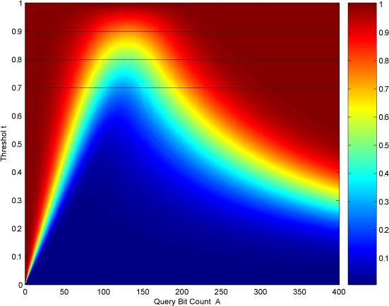
Discarded fraction f as a function of the query bit count A and the threshold t. The three lines associated with thresholds 0.7, 0.8, and 0.9 correspond to the curves in Figure 7.

7.2 Average Speedup for Single-Molecule Query as a Function of Threshold, A, and Fingerprint Length

Perhaps more important than the previous worst case analysis, is the analysis of the average speedup. We can compute the average fraction of the database to be discarded by integrating over the query molecules

$$f={\int }_{D}f\left(A\right)g_D\left(A\right)dA$$ (29)

This average can be computed with D equal to the entire database and the corresponding density g_D(B), or usingadensity g_Q(B) over queries. The latter in general gives an even more favorable speedup factor because queries tend to have a skewed distribution with respect to the database distribution, often with a smaller average value of A (Figure 9). For the average computed with g_D over the entire database, with Tanimoto similarity measure, we can again use the Gaussian approximation to g_D to obtain

$$1-f_D\approx {\int }_{A\in D}[G_D\left(\frac{A}{t}\right)-G_D\left(At\right)]g_D\left(A\right)dA$$ (30)

which can be estimated numerically. When t is close to 1, we can use the approximation in Equation 28 and integrate to get

$$1-f_D\approx \frac{\mu (1-t^2)}{2t\sigma \sqrt{\pi }}\approx \frac{\mu (1-t)}{\sigma \sqrt{\pi }}$$ (31)

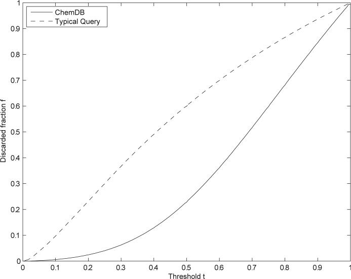
thus in this case the speedup factor grows again like C/(1 — t). Figure 9 shows how the average discarded fraction f is even larger when the average is computed over a distribution of typical queries (g_Q), rather than the database distribution (g_D).

Figure 9.

Average speedup as a function of threshold for single-molecule query using the Tanimoto similarity measure on binary compressed fingerprints of length 512. Average is computed over the ChemDB distribution using a random sample of 50,000 molecules (solid line), or over the distribution of Web queries received by the ChemDB over a period of four consecutive months (dashed line). A similarity threshold of 0.9 yields approximately a 12-fold speedup for the average query.

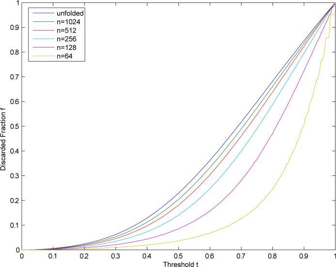
The same techniques can be applied to study other effects, such as the impact of fingerprint length on the speedup factor. Figure 10 shows how the speedup increases with the length of the fingerprints. The fingerprint bit count distribution is more concentrated for shorter fingerprints and therefore the fraction of the database discarded at a given threshold is smaller. To obtain an analytical expression, we have derived in the Appendix the following average relationship between A_* and A

$$A\approx N\left(1-{(1-\frac{A_{\ast }}{N_{\ast }})}^{N_{\ast }∕N}\right)$$ (32)

where A_* denotes the number of bits set to one in the unfolded (uncompressed) fingerprint, and N_* denotes the length of the uncompressed fingerprints. Combined with the Gaussian approximation to the distribution of A_*, this yields the distribution g_D(A) as a function of the length N of the fingerprints

$$g_D\left(A\right)\approx \frac{N}{N-A}{g}_{N_{\ast }}\left(-N\log (1-\frac{A}{N})\right)$$ (33)

where g_N* is the Gaussian approximation to the distribution over the uncompressed fingerprints of length N_*, with mean μ_* and standard deviation σ_*. Thus in this case we have

$$1-f\left(A\right)={\int }_{x_0}^{x_1}\frac{N}{N-A}{g}_{N_{\ast }}\left(-N\log (1-\frac{A}{N})\right)dA$$ (34)

With the Tanimoto measure, when t is close to 1 we get the approximation

$$1-f\left(A\right)\approx \frac{A(1-t^2)}{t}\frac{N}{N-A}{g}_{N_{\ast }}\left(-N\log (1-\frac{A}{N})\right)\approx \frac{2AN(1-t)}{N-A}\frac{1}{\sqrt{2\pi }{\sigma }_{\ast }}{e}^{-{[{\mu }_{\ast }+N\log (1-\frac{A}{N})]}^2∕2{\sigma }_{\ast }^2}$$ (35)

By averaging over the database distribution (Equation 30), the average fraction of database to be searched with Tanimoto similarity measure and similarity threshold t is given by

$$1-f_D\approx {\int }_{A\in D}[G_D\left(\frac{A}{t}\right)-G_D\left(At\right)]\frac{N}{N-A}{g}_{N_{\ast }}\left(-N\log (1-\frac{A}{N})\right)dA$$ (36)

This can be computed by using the empirical or approximate distribution G_D for fingerprints of length N. It can also be approximated using again the approximate monotonic relation between A and A_* (Equation 32) to yield

$${\int }_{A\in D}\left[G_{N_{\ast }}(-N\log (1-\frac{A∕t}{N}))-G_{N_{\ast }}(-N\log (1-\frac{At}{N}))\right]\frac{N}{N-A}{g}_{N_{\ast }}\left(-N\log (1-\frac{A}{N})\right)dA$$ (37)

When t is close to one, an analytic approximation can be derived as above. Table 1 shows that this formula is in very good agreement with empirical values, with less than 2% error at t =0.9, for values of N ranging from 64 to 1024.

Figure 10.

Average discarded fraction as a function of threshold for single-molecule query using the Tanimoto similarity measure on binary compressed fingerprints of various length. The fraction increases monotonically with the length of the fingerprints.

Table 1.

Comparison between predicted and empirical values of the curves in Figure 10 as a function of fingerprint length when the threshold approaches 1 (here t = 0.9). Predicted values are derived from Equation 37. The distribution g_N* is approximated with a Gaussian with mean=138.68, and standard deviation 53.24, estimated from the ChemDB.

N	Empirical f	Predicted Value (Equation 37)	Percent Error
1024	0.8345	0.835	0.06%
512	0.8226	0.8223	0.04%
256	0.7949	0.793	0.24%
128	0.7236	0.7148	1.22%
64	0.5057	0.4979	1.54%

7.3 Speedup for the Top K Hits

For fixed threshold searches, the speedup does not depend on the size |D| of the database. The situation is different, however, if we search for the top K hits. Using continuous notation, here we let f_A(x) and F_A(x) denote the density and distribution functions of the similarity scores (for instance Tanimoto scores) across the entire database averaged over all single-query molecules $\mathcal{A}$ satisfying the constraint Σi A_i = A. Likewise, we can consider the average f_D of f_A, computed over the entire database, and the corresponding distribution F_D. The densities f_A and f_D are typically bell-shaped over the finite [0,1] interval and therefore, to a first order of approximation, can be modeled using a Beta distribution of the form

$$\gamma x^{a-1}{(1-x)}^{b-1}=\frac{\Gamma (a+b)}{\Gamma \left(a\right)\Gamma \left(b\right)}{x}^{a-1}{(1-x)}^{b-1}$$ (38)

where a, b ≥ 0 are parameters that depend on A in the case of f_A, and γ is the normalizing constant. With a database of size |D| and a query of bit size A, the top K hits correspond to a threshold value u such that

$${\int }_u^1\gamma x^{a-1}{(1-x)}^{b-1}=\frac{K}{\mid D\mid }$$ (39)

By bounding and integrating, this gives immediately

$$\gamma u^{a-1}\frac{{(1-u)}^b}{b}\le \frac{K}{\mid D\mid }\le \gamma \frac{{(1-u)}^b}{b}$$ (40)

from which we can derive

$$u\approx 1-{\left(\frac{bK}{\gamma \mid D\mid }\right)}^{1∕b}=1-{\left(\frac{bK\Gamma \left(a\right)\Gamma \left(b\right)}{\Gamma (a+b)\mid D\mid }\right)}^{1∕b}$$ (41)

Thus, as a function of database size, the threshold u scales like [1 − C|D|^−/b]. In turn this threshold can be entered in the equations derived above, especially when the threshold approaches 1, to obtain the scaling of the speedup factor as a function of database size. For instance, by substituting this threshold in Equation 31, we get

$$1-f_D\approx \frac{u}{\sigma \sqrt{\pi }}{\left(\frac{bK\Gamma \left(a\right)\Gamma \left(b\right)}{\Gamma (a+b)\mid D\mid }\right)}^{1∕b}\approx \left(C{\mid D\mid }^{-1∕b}\right)$$ (42)

and similarly with Equation 36, when the threshold approaches 1. The fraction of database to be searched scales like C|D|^1−(1/b). Thus the fraction of the database to be searched becomes smaller and smaller as the size |D| of the database increases and the speedup factor grows like |D|^1/b.

It is worth noting that more subtle analyses are possible by modeling f_D as a mixture of two (or more) Beta distributions where, for example, one component has a large mixing coefficient and corresponds to the overwhelming majority of molecules that do not match the query, while the other component has a small mixing coefficient and corresponds to the molecules that have high similarity to the query. Since in the calculation above we are interested exclusively in the right tail of f_D near 1, the same analysis can be applied to these more complex models by focusing on the corresponding Beta component and including the mixing coefficient in the proportionality constant.

Figure 11, drawn for fingerprints of length N = 512, shows the excellent agreement between the theoretical expression (Equation 42) and the empirical values. With Tanimoto similarity, this yields values of b on the order of 2.5, thus the fraction of the database to be searched scales like O(|D|^1−(1/b) = O(|D|^0.6), with sublinear speedup.

Figure 11.

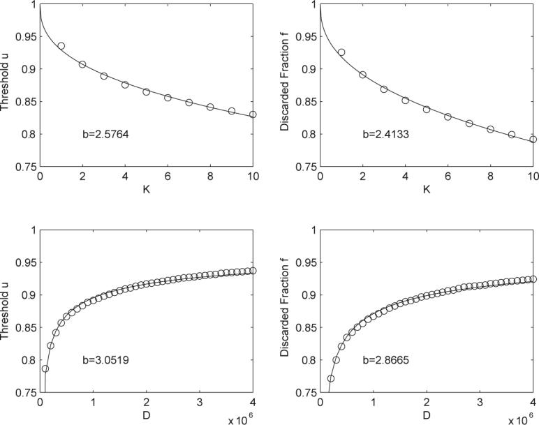
The two upper plots correspond to an experiment where K is varied and |D| is held constant at 4,099,792. Results are averaged over 5,000 separate queries randomly chosen from the ChemDB. The two lower plots correspond to an experiment where |D| is varied and K is held constant at 1, the data is averaged over 1,000 separate queries randomly chosen from ChemDB. The lines are the best fit curves using the functional form given by y = 1 − C(K/|D|)^1/b, where b and C are the fit parameters and y corresponds either to u or the fraction pruned from the database. This equation fits the data very closely with similar values for b. One can notice a small, but systematic, misfit between the empirical points and the theoretical curve y = 1 − C(K/|D|)^1/b. This can be entirely eliminated by introducing one additional offset parameter and fitting y = 1 − [C₁ + C₂(K/|D|)^1/b] to the data.

While the simulation results show that these scaling formula hold for current database sizes with millions of chemicals, it is clear that the scaling breaks downs as |D| → ∞ simply because of the discrete nature of the bins associated with the values of B. For extremely large values of |D|, the top K molecules $\mathcal{B}$ that are most similar to a query molecule $\mathcal{A}$ must be in the same bin as $\mathcal{A}$ and must satisfy B = A. Therefore, once the database is large enough to reach this regime, by the current methods one must search all the molecules contained in the same bin as $\mathcal{A}$ and the speedup becomes linear again, i.e. one needs to search P_N (A)|D| records. It is possible to estimate the size D*(N) of the database at which this regime takes over. Clearly, D* depends on the fingerprint length N and increases with N. To estimate D* based on average case analysis, we notice that when the linear regime is in effect, for a query $\mathcal{A}$ we need to search a fraction P_N (A) of molecules, thus on average we need to search a fraction of the database equal to

$$\varphi \left(N\right)=\sum _A{P}_N{\left(A\right)}^2$$ (43)

and discard the fraction 1 − φ. We can then apply this value on the y axis of the curves in Figure 10 or 11 to find the correponding value of |D|. Using the curves and equations of Figure 11, this gives φ(N) = C(K/D*(N))^1/b or φ(N) = C₁ + C₂(K/D*(N))^1/b resulting in

$$D^{\ast }\left(N\right)\approx K{\left(\frac{C}{\varphi \left(N\right)}\right)}^b\text{or}{D}^{\ast }\left(N\right)\approx K{\left(\frac{C_2}{(\varphi \left(N\right)-C_1)}\right)}^b$$ (44)

For N = 512 and the values in Figure 11, we get φ = 0.0032 and |D|/K = 6.7268e + 07, using the more accurate model with offset. Thus the equations predict that the speedup will transition from sublinear to linear when D*(N) is about 67 million compounds with K = 1, and 670 million compounds when K = 10. These estimates are sensitive to the values of the Cs and b and therefore should only be considered as indicative. However, they clearly indicate that for the foreseeable future the speedup will remain sublinear, and this is even more true with longer fingerprints, of length N = 1024 and beyond, which are widely used.

8 Conclusion

Current fingerprint search systems often require sequentially scanning the entire fingerprint database. While this search strategy works for small to moderately sized databases which can be stored in memory, it does not scale up well. In most practical applications, the user is not interested in computing all similarity values but only the top hits, and perhaps estimating the histogram of the entire distribution of similarity scores. Here we have shown how using pre-stored information about the number of bits set to one in each binary fingerprint, or the total number of counts in a non-binary fingerprint, we can greatly restrict the number of compounds for which a similarity score must be computed.

The method uses simple mathematical bounds on fingerprint similarity measures to search only a fraction of the database using the prestored information. With searches involving a fixed linear threshold, the method yields linear speedup where one needs to search only a fraction (1 − f) of the database. We have shown how the factor 1 − f depends on threshold and fingerprint length, and can lead to speedups of one order of magnitude or more. With searches aimed at retrieving the top K hits, the method yields even better sublinear speedups where, in a typical case, the fraction of database to be searched scales like |D|^0.6. The method requires no tuning and remains exact in the sense that it returns the same results as if the entire database was searched. As shown in the benchmark experiments reported in Table 2, when applied to the 5M compounds in the ChemDB the method delivers subsecond searchtimes on a single desktop machine.

Table 2.

Actual search time benchmarks obtained searching the entire ChemDB database, with about 5M compounds using a 2.4MHz AMD Opteron processor with 2 GB of memory. Searches are carried using Tanimoto similarity measure with threshold (t = 0.9), or top ten (K = 10), or both. Search times for single-molecule query are expressed in seconds and are averaged over each dataset. The datasets correspond to the six Stahl and Rarey¹⁴ datasets, a random set of 1,000 queries extracted from the set of actual ChemDB queries, and a random set of 100 queries taken from the ChemDB. The fraction of the database that needs to be searched is given by 1 — f.

Dataset	Size	Time (t=0.9)	1-f	Time (K=10)	1-f	Time (t=0.9,K=10)	1-f
Cox2	128	0.79	0.17	3.53	0.76	0.78	0.17
Estrogen	55	0.60	0.12	2.03	0.43	0.52	0.11
Gelatinase A	43	0.77	0.16	3.31	0.71	0.77	0.16
Neuraminidase	17	0.70	0.14	2.74	0.59	0.66	0.14
p38 MAP kinase	25	0.90	0.18	3.30	0.71	0.87	0.18
Thrombin	67	0.91	0.19	3.27	0.70	0.88	0.19
ChemDB Queries	1,000	0.27	0.06	1.12	0.24	0.26	0.06
Random ChemDB	100	0.64	0.14	1.23	0.27	0.58	0.12

Appendix A: Extensions to Other Similarity Measures

Fingerprint similarity can be calculated using many different measures. Holliday et al. (2002)¹⁸ compare a comprehensive list of fingerprint similarities and distances. Using their nomenclature, we show here how to calculate bounds on these measures, essentially by expressing each measure in terms of unions and intersections, studying the corresponding derivatives, and applying corresponding bounds.

As previously derived, the Jaccard/Tanimoto measure is defined as, and bounded by,

$$S(\overrightarrow{A},\overrightarrow{B})=\frac{A\cap B}{A\cup B}\le T(A,B)=\frac{\min (A,B)}{\max (A,B)}$$ (45)

The Baroni-Urbani/Buser measure is similar to the Jaccard/Tanimoto measure, and is defined as

$$S(\overrightarrow{A},\overrightarrow{B})=\frac{\sqrt{(A\cap B)(N-A\cup B)}+A\cap B}{\sqrt{(A\cap B)(N-A\cup B)}+A\cup B}$$ (46)

and using the identity min(A, B) max (A, B) = AB we can derive the bound

$$S(\overrightarrow{A},\overrightarrow{B})\le T(A,B)=\frac{\sqrt{N\min (A,B)-AB}+\min (A,B)}{\sqrt{N\min (A,B)-AB}+\max (A,B)}$$ (47)

Closely related to the Jaccard/Tanimoto measure, the Ochiai/Cosine measure is defined as, and bounded by,

$$S(\overrightarrow{A},\overrightarrow{B})=\frac{A\cap B}{\sqrt{AB}}\le T(A,B)=\frac{\min (A,B)}{\sqrt{AB}}$$ (48)

Also closely rrelated to the Jaccard/Tanimoto measure, the Pearson measure is defined as

$$S(\overrightarrow{A},\overrightarrow{B})=\frac{N(A\cap B)-AB}{\sqrt{AB(N-A)(N-B)}}$$ (49)

and bounded by

$$S(\overrightarrow{A},\overrightarrow{B})\le T(A,B)=\frac{N\min (A,B)-AB}{\sqrt{AB(N-A)(N-B)}}$$ (50)

The rather complex Stiles measure produces nearly identical rankings as the Pearson measure. It is defined as

$$S(\overrightarrow{A},\overrightarrow{B})={\log }_{10}\frac{N{(\mid N(A\cap B)-AB\mid -\frac{N}{2})}^2}{AB(N-A)(N-B)}$$ (51)

and bounded by

$$S(\overrightarrow{A},\overrightarrow{B})\le T(A,B)={\log }_{10}\frac{N{(N\min (A,B)-AB-\frac{N}{2})}^2}{AB(N-A)(N-B)}$$ (52)

The McConnaughey and Dennis measures also are both closely correlated with the Jaccard/Tanimoto measure. The McConnaughey measure is defined as

$$S(\overrightarrow{A},\overrightarrow{B})=\frac{(A\cap B)(2-A-B)+AB}{AB}$$ (53)

and bounded by

$$S(\overrightarrow{A},\overrightarrow{B})\le T(A,B)=\frac{\min (A,B)(2-A-B)+AB}{AB}$$ (54)

While the Dennis measure is defined as, and bounded by,

$$S(\overrightarrow{A},\overrightarrow{B})=\frac{N(A\cap B)-AB}{\sqrt{NAB}}\le T(A,B)=\frac{N\min (A,B)-AB}{\sqrt{NAB}}$$ (55)

Perhaps the simplest measure, Russel/Rao, performs surprisingly well: in some tests better than the more commonly used Jaccard/Tanimoto measure. It is defined as, and bounded by,

$$S(\overrightarrow{A},\overrightarrow{B})=\frac{A\cap B}{N}\le T(A,B)=\frac{\min (A,B)}{N}$$ (56)

The Dice and Sokal/Sneath(1) measures are equivalent to the Tversky similarity measure with α = β = 0.5 and α = β = 2 respectively. Noting this relationship, we can use the bounds on the Tversky similarity to derive bounds on these measures. For example, for the Dice measure we have

$$S(\overrightarrow{A},\overrightarrow{B})=\frac{2(A\cap B)}{A+B}\le T(A,B)=\frac{2\min (A,B)}{A+B}$$ (57)

The Sokal/Sneath(2) measure is defined as

$$S(\overrightarrow{A},\overrightarrow{B})=\frac{2(N-A-B+2(A\cap B))}{2N-A-B+2(A\cap B)}$$ (58)

Using the identity A + B − 2 min(A, B) = |A − B| we can derive its bound

$$S(\overrightarrow{A},\overrightarrow{B})\le T(A,B)=\frac{2N-2\mid A-B\mid }{2N-\mid A-B\mid }$$ (59)

We can use the same identity to define and bound the Sokal/Sneath(3) measure

$$S(\overrightarrow{A},\overrightarrow{B})=\frac{N-A-B+2(A\cap B)}{A+B-2(A\cap B)}\le T(A,B)=\frac{N-\mid A-B\mid }{\mid A-B\mid }$$ (60)

Similarly, the Simple Matching measure, which can also be viewed as the complement of the Mean Manhattan Distance, is defined as, and bounded by,

$$S(\overrightarrow{A},\overrightarrow{B})=\frac{N-A-B+2(A\cap B)}{N}\le T(A,B)=\frac{N-\mid A-B\mid }{N}$$ (61)

Similarly, the Kulczynski(1) measure is defined as, and bounded by,

$$S(\overrightarrow{A},\overrightarrow{B})=\frac{A\cap B}{A+B-2(A\cap B)}\le T(A,B)=\frac{\min (A,B)}{\mid A-B\mid }$$ (62)

Using again the identity $\frac{\min (A,B)}{\left(AB\right)}=\frac{1}{\max (A,B)}$, the Kulczynski(2) measure is defined as, and bounded by,

$$S(\overrightarrow{A},\overrightarrow{B})=\frac{(A\cap B)(A+B)}{2AB}\le T(A,B)=\frac{A+B}{2\max (A,B)}$$ (63)

Similarly, the Hamann measure is defined as, and bounded by,

$$S(\overrightarrow{A},\overrightarrow{B})=\frac{N+4(A\cap B)-2A-2B}{N}\le T(A,B)=\frac{N-2\mid A-B\mid }{N}$$ (64)

The Rogers/Tanimoto measure is similar to the Sokal/Sneath(3) measure. It is defined as, and bounded by,

$$S(\overrightarrow{A},\overrightarrow{B})=\frac{N-A-B+2(A\cap B)}{N+A+B-2(A\cap B)}\le T(A,B)=\frac{N-\mid A-B\mid }{N+\mid A-B\mid }$$ (65)

The Forbes measure is defined as, and bounded by,

$$S(\overrightarrow{A},\overrightarrow{B})=\frac{N(A\cap B)}{AB}\le T(A,B)=\frac{N}{\max (A,B)}$$ (66)

Closely correlated with the Forbes measure, the Yule measure is defined as

$$S(\overrightarrow{A},\overrightarrow{B})=\frac{N(A\cap B)-AB}{(A\cap B)(N-2A-2B+2)+AB}$$ (67)

and bounded by

$$S(\overrightarrow{A},\overrightarrow{B})\le T(A,B)=\frac{N\min (A,B)-AB}{\min (A,B)(N-2A-2B+2)+AB}=\frac{N-\max (A,B)}{N-2A-2B+2+\max (A,B)}$$ (68)

The Fossum measure is defined and bounded by

$$S(\overrightarrow{A},\overrightarrow{B})=\frac{N{((A\cap B)-0.5)}^2}{AB}\le T(A,B)=\frac{N{(\min (A,B)-0.5)}^2}{AB}$$ (69)

The Simpson measure is defined as

$$S(\overrightarrow{A},\overrightarrow{B})=\frac{A\cap B}{\min (A,B)}$$ (70)

In this case, the obvious upperbound is 1 and it is achieved when A ≤ 0 and B ≤ 0.

$$S(\overrightarrow{A},\overrightarrow{B})\le T(A,B)=\frac{\min (A,B)}{\min (A,B)}=1$$ (71)

This upperbound does not lead to any search space reduction.

In some applications, such as selecting a diverse dataset, one is interested in minimizing similarity (or maximizing distance) instead. This approach is meaningful only with certain metrics. To maximize distance between fingerprints we must minimize the overlap between $\overrightarrow{A}$ and $\overrightarrow{B}$, and so we can lower bound ($A\cap B$) with max(A + B − N, 0), the minimum possible overlap. For example, this can be applied to the Mean Manhattan distance, which is also the L1 norm or the city-block distance. It is the the complement of the Simple Matching measure and, in the binary case, it is rank-equivalent to Euclidian distance. It is defined as, and bounded by,

$$S(\overrightarrow{A},\overrightarrow{B})=\frac{A+B-2(A\cap B)}{N}\le T(A,B)=\frac{A+B-2\max (A+B-N,0)}{N}$$ (72)

Similarly, the Normalized Euclidian distance is the familiar L2 norm, defined as

$$S(\overrightarrow{A},\overrightarrow{B})=\sqrt{\frac{A+B-2(A\cap B)}{N}}$$ (73)

It can be bounded in the same way by

$$S(\overrightarrow{A},\overrightarrow{B})\le T(A,B)=\sqrt{\frac{A+B-2\max (A+B-N,0)}{N}}$$ (74)

In short, we have shown how the same principles can be applied essentially to all the other fingerprint similarity/distance measures that are found in the literature.

Appendix B: Estimation A Given A_*

To estimate A from A_*, we assume that the order of the bits in the long uncompressed fingerprints has been randomized, so that we can use a simple binomial approximation where we assume that the bits in the uncompressed fingerprints are set to one according to a binomial coin flip process B(N_*,α) with probability α = A_*/N_*. Then with modulo compression the probability of setting a given bit to zero in the compressed $\overrightarrow{A}$ is (1 − α)^k, where k = N_*/N. Therefore the corresponding distribution for A is binomial B(N, p)with:

$$P(A\mid \alpha )=\mathcal{B}(n,p)\text{with}p=1-{(1-\alpha )}^k$$ (75)

Therefore, given α (or A_*)

$$E(A\mid \alpha )=N[1-{(1-\alpha )}^k]$$ (76)

Thus, given A_*, we can estimate A by

$$E(A\mid A_{\ast })\approx N[1-{(1-\frac{A_{\ast }}{N_{\ast }})}^{N_{\ast }∕N}]$$ (77)

Asymptotically, for large N_*, we can use

$$E(A\mid A_{\ast })\approx N(1-e^{-A_{\ast }∕N})$$ (78)

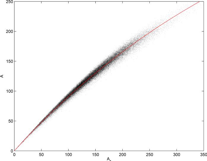
Equations 77 and 78 provide very good approximations to the true value, as shown in Figure 12.

Figure 12.

Each point represents a molecule in the random subset of 50,000 molecules from the ChemDB, using binary fingerprints of length N = 512. Random jitter uniform over [−0.5,0.5] is injected in each coordinate to improve readability. The red curve corresponds to the predicted relationship between A and A_* using the asymptotic approximation to the binomial model (Equation 78). The predicted values correspond closely to the expected empirical values

References

- 1.Irwin JJ, Shoichet BK. ZINC–a free database of commercially available compounds for virtual screening. J. Chem. Inf. Comput. Sci. 45:177–182. doi: 10.1021/ci049714. [DOI] [PMC free article] [PubMed] [Google Scholar]
- 2.Chen J, Swamidass SJ, Dou Y, Baldi P. ChemDB: a public database of small molecules and related chemoinformatics resources. Bioinformatics. 2005;21:4133–4139. doi: 10.1093/bioinformatics/bti683. [DOI] [PubMed] [Google Scholar]
- 3.Fligner MA, Verducci JS, Blower PE. A Modification of the Jaccard/Tanimoto Similarity Index for Diverse Selection of Chemical Compounds Using Binary Strings. Technometrics. 2002;44:110–119. [Google Scholar]
- 4.Flower DR. On the properties of bit string-based measures of chemical similarity. J. Chem. Inf. Comput. Sci. 1998;38:378–386. [Google Scholar]
- 5.James CA, Weininger D, Delany J. “Daylight Theory Manual”. Daylight Theory Manual, 2004. 2004 Available at http://www.daylight.com/dayhtml/doc/theory/theory.toc.html. [Google Scholar]
- 6.Xue L, Godden JF, Stahura FL, Bajorath J. Profile scaling increases the similarity search performance of molecular fingerprints containing numerical descriptors and structureal keys. J. Chem. Inf. Comput. Sci. 2003;43:1218–1225. doi: 10.1021/ci030287u. [DOI] [PubMed] [Google Scholar]
- 7.Xue L, Stahura FL, Bajorath J. Similarity search profiling reveals effects of fingerprint scaling in virtual screening. J. Chem. Inf. Comput. Sci. 2004;44:2032–2039. doi: 10.1021/ci0400819. [DOI] [PubMed] [Google Scholar]
- 8.Bohacek RS, McMartin C, Guida WC. The art and practice of structure-based drug design: a molecular modelling perspective. Medicinal Research Reviews. 1996;16:3–50. doi: 10.1002/(SICI)1098-1128(199601)16:1<3::AID-MED1>3.0.CO;2-6. [DOI] [PubMed] [Google Scholar]
- 9.Tversky A. Features of similarity. Psychological Review. 1977;84:327–352. [Google Scholar]
- 10.Rouvray D. Definition and role of similarity concepts in the chemical and physical sciences. J. Chem. Inf. Comput. Sci. 1992;32:580–586. [Google Scholar]
- 11.Swamidass SJ, Chen J, Bruand J, Phung P, Ralaivola L, Baldi P. Kernels for small molecules and the prediction of mutagenicity, toxicity, and anti-cancer activity. Bioinformatics. 2005;21:i359–368. doi: 10.1093/bioinformatics/bti1055. [DOI] [PubMed] [Google Scholar]
- 12.van Rijsbergen CJ. Information Retrieval. Information Retrieval. Butterworths; London, UK: 1978. [Google Scholar]
- 13.Ralaivola L, Swamidass SJ, Saigo H, Baldi P. Graph kernels for chemical informatics. Neural Networks. 2005;18:1093–1110. doi: 10.1016/j.neunet.2005.07.009. [DOI] [PubMed] [Google Scholar]
- 14.Stahl M, Rarey M. Detailed analysis of scoring funtions for virtual screening. J. Med. Chem. 2001;44:1035–1042. doi: 10.1021/jm0003992. [DOI] [PubMed] [Google Scholar]
- 15.Downs GM, Gillet VJ, Holliday JD, Lynch MF. Computer storage and retrieval of generic chemical structures in patents. 10. The generation and logical bubble-up of ring screens for structurally-explicit generics. J. Chem.Inf.Comput. Sci. 1989;29:215–224. [Google Scholar]
- 16.Shemetulskis NE, Weininger D, Blankley CJ, Yang JJ, Humblet C. Stigmata: an algorithm to determine structural commonalities in diverse datasets. J. Chem. Inf. Comput. Sci. 1996;36:862–871. doi: 10.1021/ci950169+. [DOI] [PubMed] [Google Scholar]
- 17.Wild DJ, Blankley CJ. VisualiSAR: a web-based application for clustering, structure browsing, and structure-activity relationship study. J. Mol. Graph. Model. 1999;17:85–89. 120–125. doi: 10.1016/s1093-3263(99)00026-1. [DOI] [PubMed] [Google Scholar]
- 18.Holliday JD, Hu CY, Willett P. Grouping of coefficients for the calculation of inter-molecular similarity and dissimilarity using 2d fragment bit-strings. Comb. Chem. High Throughput Screen. 2002;5:155–166. doi: 10.2174/1386207024607338. [DOI] [PubMed] [Google Scholar]