

Abstract
A major challenge in functional neuroimaging is to cope with individual variability in cortical structure and function. Most analyses of cortical function compensate for variability using affine or low-dimensional nonlinear volume-based registration (VBR) of individual subjects to an atlas, which does not explicitly take into account the geometry of cortical convolutions. A promising alternative is to use surface-based registration (SBR), which capitalizes on explicit surface representations of cortical folding patterns in individual subjects. In this study, we directly compare results from SBR and affine VBR in a study of working memory in healthy controls and patients with schizophrenia (SCZ). Each subject's structural scan was used for cortical surface reconstruction using the SureFit method. fMRI data were mapped directly onto individual cortical surface models, and each hemisphere was registered to the population-average PALS-B12 atlas using landmark-constrained SBR. The precision with which cortical sulci were aligned was much greater for SBR than VBR. SBR produced superior alignment precision across the entire cortex, and this benefit was greater in patients with schizophrenia. We demonstrate that spatial smoothing on the surface provides better resolution and signal preservation than a comparable degree of smoothing in the volume domain. Lastly, the statistical power of functional activation in the working memory task was greater for SBR than for VBR. These results indicate that SBR provides significant advantages over affine VBR when analyzing cortical fMRI activations. Furthermore, these improvements can be even greater in disorders that have associated structural abnormalities.
Introduction
Cortical Alignment Accuracy
One of the main challenges in fMRI studies is to optimize the alignment of anatomical and functional data across individuals. Currently, most fMRI studies use a volumetric representation for data analysis (Friston et al., 1995; Worsley and Friston., 1995; Acton and Friston, 1998) and apply volume based registration (VBR) to compensate for individual variability (Woods et al, 1998). Although the most widely used affine VBR and low-dimensional nonlinear (LDN) VBR methods (Cox, 1996; Jenkinson & Smith, 2001; Jenkinson et al., 2002) do reduce intersubject variability (Woods et al, 1998) and are geometrically appropriate for most subcortical structures, high cortical 3D variability presents a real alignment challenge. Human cortex is essentially a 2D folded sheet of tissue whose deep folds allow a large surface area to fit inside the skull. Owing to this geometric arrangement, some functionally distant structures are closely apposed in volume space (e.g. the opposing banks of every deep sulcus). The high variability of folding patterns across individuals limits the degree of alignment of cortical regions attainable with affine and LDN VBR, since these approaches are largely oblivious to the detailed folding pattern of each person's cortex (Woods et al, 1998; Van Essen, 2005; Van Essen and Dierker, 2007). An attractive strategy is to capitalize on surface models from individual structural MRI volumes that can be generated using various software packages (e.g. Freesurfer - Fischl et al., 1999a; Brain Voyager – Goebel, 1996, 1997; and Caret-Van Essen et al., 2001). Surface models lend themselves to surface-based registration (SBR) techniques, which in theory are better suited to account for each person's cortical folding pattern (Dale et al., 1999; Fischl et al., 1999; Van Essen, 2005). For example, landmark-based SBR to the PALS atlas achieves superior results when compared to affine or LDN VBR in aligning cortical sulci throughout each hemisphere (Van Essen, 2005).
Spatial Smoothing
Spatial smoothing (blurring) is commonly applied to fMRI data to increase signal-to-noise ratio (SNR, Cox, 1996), but inevitably at the expense of spatial resolution. Smoothing of volume fMRI data is typically the same along each axis and is thus isotropic from a volumetric perspective. However, volume-based smoothing is highly anisotropic and irregular from a surface-based perspective, because neighboring voxels in 3D space often represent locations that are distant in cortical (2D) space. Using synthetic fMRI data, Jo et al. (2007) placed activations on the anterior bank of the central sulcus and applied smoothing in 3D (volume) and 2D (surface) using a Gaussian kernel. With 3D smoothing they demonstrated substantial spread of activation onto the posterior bank of the sulcus even at low smoothing (4 mm kernel). No such ‘bleeding’ occurred even at a maximum smoothing strength of 10 mm when the synthetic data were smoothed on the surface. Here, we demonstrate a similar outcome using actual fMRI data.
Power in fMRI Analysis
In volume-averaged analyses of group fMRI data, statistical power depends on both the strength of the signal in individual subjects, and on the consistency of the signal across individuals within the group. If the activation patterns from individuals are brought into better alignment, the mean signal should be increased and the variability of the signal across individuals reduced, thereby enhancing statistical power. Previous work using synthetic fMRI showed that surface-based analysis can improve statistical power (Andrade et. al, 2001; Jo et al., 2007). Studies using SBR registration techniques with actual fMRI signals have shown superior power when compared to VBR analyses (Fischl et al., 1999; Desai et al, 2005; Argall et al., 2006). However, these earlier investigations were either limited in the extent of cortex analyzed (e.g., Desai et al., 2005 examined only auditory cortex) or involved a suboptimal VBR registration. (e.g., Argall et al., 2006 used piecewise linear registration to Talairach and Tournoux space). The present study compares affine-based VBR with landmark-based SBR approach across widespread cortical regions activated by working memory tasks.
Populations with Structural Deficits
The challenge of aligning brain anatomy across individuals encounters additional issues when dealing with patient populations having abnormalities in brain structure. For example, individuals with schizophrenia (SCZ) show subtle abnormalities of both volume and shape in a number of regions, including the hippocampal complex, prefrontal cortex and multiple subcortical nuclei (Shenton et al., 2001). Such structural abnormalities could, in principle, reduce the fidelity of structural alignment across individuals. This might in turn lead to an apparent reduction in activation strength among individuals with SCZ that instead reflects reduced alignment fidelity. Increased alignment fidelity and power of fMRI analyses with SBR as compared to VBR might therefore impact the interpretation of fMRI results with clinical populations.
Working Memory as a Functional Task
Previous SBR analyses have focused on sensory and motor processing in healthy individuals (Fischl et al., 1999; Desai et al., 2005; Argall et al., 2006). It is useful to compare SBR and VBR analyses using cognitive tasks that activate a broader domain of cortical regions. The current study focuses on working memory, since it is a well-studied cognitive process that engages a range of cortical regions (Badelley, 1986; D'Esposito et al., 1995; Barch et al., 2002; Braver et al., 2001;) and is impaired in schizophrenia (Goldman-Rakic, 1994; Barch et al., 2001). Examining working memory in schizophrenia provides a good test-bed for addressing whether patient populations with subtle structural abnormalities may show enhanced benefit from SBR.
The current study tests three main hypotheses: 1) Is the improved alignment of identified sulci using landmark-based SBR compared to affine VBR (Van Essen, 2005) even greater for individuals with SCZ than for healthy controls? 2) Does 2D (surface) spatial smoothing of real fMRI data preserve the location of activation peaks more accurately than Gaussian smoothing applied in 3D? 3) Are fMRI power profiles in a cognitive task stronger for landmark-based SBR than for affine VBR and is the benefit greater for the SCZ than the healthy control group? Issues related to alternative VBR and SBR methods that were not explored in the present study are considered in the Discussion.
Materials and Methods
Subjects
Subjects were recruited through the clinical core of the Conte Center for Neuroscience of Mental Disorders (CCNMD) at Washington University in St. Louis as part of two separate study protocols (described below) with identical subject selection criteria. Clinical assessments were conducted by a research associate trained to administer the SCID-IV, who also regularly participated in diagnostic rating sessions. An additional assessment session was conduced by an expert clinician using a semi-structured interview for DSM-IV as well as all available patient records. A consensus on each diagnosis was reached between the interviewer and the expert clinician. The complete sample included 29 subjects (11 from protocol A and 18 from protocol B) meeting DSM-IV diagnostic criteria for schizophrenia (SCZ) and 30 (10 from protocol A and 20 from protocol B) demographically matched healthy control (CTRL) subjects (for complete demographic information see Table 1.). CTRL subjects for both protocols were recruited using local advertisements in the same community from which SCZ subjects were recruited. CTRL subjects were not included in either of the two protocols if they had any lifetime history of Axis I psychiatric disorder or a first-degree relative with a psychotic disorder. Both CTRL and SCZ subjects were also excluded from either protocol if they 1) met criteria for DSM-IV substance abuse or dependence within the past 6 months; 2) they had any severe medical complications that would compromise psychiatric assessment and diagnosis or render the subject unstable or at risk to participate; 3) they suffered head injury (past or present) with manifestation of neurological symptoms of loss of consciousness or 4) met DSM-IV diagnostic criteria of mental retardation. All SCZ subjects were taking antipsychotic medication at the time of the scan and in order to be included in the study SCZ subjects had to be stable for a period of at least 2 weeks. All subjects completed and signed an informed consent approved by the Washington University Institutional Review Board. All subjects were assessed for handedness using the Edinburgh Handedness Inventory (Oldfield, 1971). Given identical cognitive tasks and recruitment criteria for the two protocols, we pooled the data for the purposes of the current study to increase sample size while eliminating a balanced contribution of SCZ and CTRL across both protocols.
Table 1.
Demographics and clinical data
| Characteristic | Controls |
Schizophrenia |
Significance |
|||
|---|---|---|---|---|---|---|
| M | S.D. | M | S.D. | T Value/Chi-Square | P Value | |
| Age (in years) | 26.55 | 11.74 | 27.10 | 9.70 | −0.2 | 0.84 |
| Gender (% male) | 66.67 | 79.31 | 1.084 | 0.283 | ||
| Parent's education (in years) | 14.33 | 2.50 | 13.96 | 3.79 | 0.44 | 0.67 |
| Participant's education (in years) | 13.45 | 2.74 | 11.95 | 2.52 | 2.21 | 0.03 |
| Handedness (% right) | 90.00 | 89.66 | 0.97 | 0.65 | ||
| Mean SAPS Global Item Score | 0.04 | 0.12 | 1.34 | 0.79 | ||
| Mean SANS Global Item Score | 0.23 | 0.25 | 1.82 | 0.76 | ||
| Disorganization | 0.90 | 1.09 | 3.69 | 2.54 | ||
| Poverty | 0.37 | 0.57 | 7.10 | 3.10 | ||
| Reality Distortion | 0.07 | 0.27 | 3.69 | 2.54 | ||
| Verbal WM Accuracy | 0.96 | 0.04 | 0.91 | 0.10 | ||
| Non-Verbal WM Accuracy | 0.93 | 0.07 | 0.87 | 0.10 | ||
| Verbal WM RT | 783.54 | 141.80 | 936.65 | 201.31 | ||
| Non-Verbal WM RT | 892.53 | 158.80 | 908.06 | 204.82 | ||
Cognitive Task
The cognitive activation task was a “2-back” version of the n-back task. The data for the 2-back task came from two larger protocols. In protocol ‘A‘ a series of 2-back runs were completed, following different types of mood induction (positive, negative and neutral emotion conditions) designed to examine emotion regulation in SCZ and CTRL (Gray et al., 2002). The current analysis used only the neutral mood induction data. Protocol ‘B’ examined working memory and episodic memory in individuals with SCZ and CTRL participants; it did not include mood manipulation. The 2-back tasks and the stimuli were identical across the two studies.
The 2-back task consisted of word or face stimuli presented on a screen, appearing one at a time. Subjects were instructed to press a button (target) every time they detected a stimulus that was the same as the one seen two stimuli back and a different button if not. Verbal stimuli were concrete English nouns that varied between 3−10 letters in length. Face stimuli were unfamiliar faces (Barch et al., 2002; Braver et al., 2001; Kelley et al., 1998; Logan et al., 2002) that were difficult for subjects to verbally label. At the beginning of each 2-back task four fixation trials were included and later discarded in order to allow for tissue magnetization to reach a steady state. Each of the two 2-back runs (one word and one face) lasted 4.25 min and included four task blocks (16 trials) and 3 fixation blocks (10 trials) interleaved. Each item within a 2-back task block was presented on the screen for 2 s and was followed by a 500 ms interstimulus interval. Visual stimuli were generated on PsyScope software (designed and developed by Cohen et al., 1993) installed on an Apple PowerMac. The order of 2-back tasks (word vs. face) was counterbalanced across subjects. The controls were more accurate and faster than individuals with schizophrenia for both word and face working memory tasks (see Supplementary Material).
Scanning
The 21 subjects from protocol A (11 SCZ and 10 CTRL, all in protocol ‘A’) were scanned on a 3T Allegra scanner at the Research Imaging Center of the Mallinckrodt Institute of Radiology at the Washington University Medical School. Functional images were acquired using an asymmetric spin-echo, echo-planar sequence, which was maximally sensitive to blood oxygenation level-dependent (BOLD) contrast (T2*) (repetition time [TR] = 2500 ms, echo time [TE] 24 ms, field of view [FOV] = 24 cm, flip=90°). Each run contained 102 sets of oblique axial images, which were acquired parallel to the anterior-posterior commissure. Each image volume contained 32 slices (4 × 4 × 4 mm resolution). The 38 subjects from protocol B (18 SCZ and 20 CTRL all in protocl ‘B’) were scanned on a on the 1.5T VISION system (TR=2500 ms, TE=50 ms, FOV=24 cm, flip=90°). Runs also contained 102 sets of oblique axial images, with 19 slices (3.75 × 3.75 × 7 mm resolution). All structural images were acquired on a 1.5T Siemens VISION system using a coronal MP-RAGE 3D T1-weighted sequence (TR=9.7 ms, TE=4 ms, flip=10°; voxel size=1× 1× 1.2 mm). Because there were no significant differences between the 1.5T and 3T datasets in terms of SNR, registration quality, or activation patterns (see Supplementary Material), we considered it justifiable to pool the data from the two scanners.
Data Preprocessing
Structural and functional magnetic resonance imaging data preprocessing steps included: 1) compensation for slice-dependent time shifts; 2) elimination of odd/even slice intensity differences due to interpolated acquisition; 3) realignment of data acquired in each subject within and across runs to compensate for rigid body motion (Ojemann et al., 1997); 4) intensity normalization to a whole brain mode value of 1,000 but without bias or gain field correction; 5) VBR of anatomical data to atlas space (see below); and 6) VBR of functional data to anatomical data (see below).
Volume Based Registration (VBR)
The entire 3D structural volume (T1) was registered to 711−2B stereotaxic atlas space using 12-parameter affine transform and resampled to 1mm cubic representation (Ojemann et al., 1997; Buckner et al., 2004). Likewise, the entire 3D fMRI volume was coregistered to the structural image acquired from 1.5T scanner and transformed to atlas space using a single affine 12-parameter transform and resampled to a 3 mm cubic representation, i.e., at a finer grain than the original acquisitions. Importantly, functional data acquired on the 3T system were aligned with their individual structural images acquired on the 1.5T system.
FMRI Analysis
A general linear model (GLM) approach was used to estimate magnitudes of task-related activity in each voxel. We convolved a box-car function with a canonical hemodynamic response and separately estimated the activation for each stimulus type (i.e. word and face working memory). Each estimate was expressed in percent change units relative to baseline for that voxel across all trials of a given stimulus type. For each stimulus type (e.g. word working memory) analyses were carried out on the unsmoothed magnitude estimates for each subject and on data spatially smoothed in the volume representation using a 9 mm full-width at half maximum (FWHM) Gaussian filter. These magnitude estimates were mapped onto the corresponding individual cortical surface models and analyzed using voxel-based and surface-based t-tests.
Surface Analysis Protocol
Segmentation
Surface-based analyses were carried out using Caret 5.5 software (http://brainmap.wustl.edu/caret/). Application of the SureFit algorithm in Caret yielded a segmentation whose boundary ran approximately midway through the cortical thickness (Fig. 1A), thereby providing a balanced representation of both sulcal and gyral regions (Van Essen et al., 2001).
Figure 1. The general workflow that was used for SBR analysis strategy.
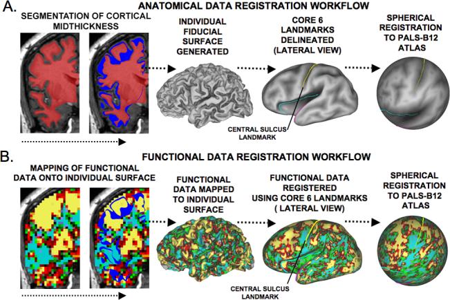
(A) Structural data is used for segmentation of cortical midthickness and a surface outline is created (blue ribbon). A fiducial surface representation is generated and Core-6 sulcal landmarks are outlined and are shown on the inflated surface representation. The Core-6 landmarks are used for spherical registration to the PALS-B12 atlas. (B) fMRI data that intersect the fiducial surface outline are first mapped onto corresponding nodes of the subject's surface model and then deformed to the PALS-B12 atlas using the same information obtained from spherical registration of anatomical data.
The automated error correction in Caret eliminated most segmentation errors. Subsequent manual correction was carried out by two trained raters [SKG and AA] and visually inspected for accuracy. The final segmentation was used to generate a ‘fiducial’ surface (Fig. 1A) that was inflated, flattened, and mapped to a spherical representation (with distortions reduced by multi-resolution morphing). Maps of cortical geography (gyral vs sulcal cortex) were generated automatically by intersecting the fiducial surface with an eroded (by 4mm) version of the ‘cerebral hull’ segmentation – a volume whose boundary runs along gyral crowns and does not dip into sulci.
Surface Based Registration (SBR)
SBR was carried out using a set of six cortical landmarks (Fig. 1A) (http://brainvis.wustl.edu/help/landmarks_core6/landmarks_core6.html/; Van Essen, 2005). To avoid inter-rater bias, all landmark delineation was done by a single trained rater [SKG]. Consistent criteria were applied to all cortical landmarks across subjects. Each hemisphere was registered to the standard spherical mesh of the PALS-B12 left-right composite atlas based on 12 normal young adults (Van Essen, 2005). As part of the registration process, each subject's fiducial surface was resampled into a standard mesh consisting of 73,730 surface nodes, which allowed both individual and group data visualization in a common reference frame (Fig. 1A). Figure 1B shows an example of the single-subject fMRI activation mapped to each of these surface configurations.
Surface and Volume Delineation of Sulci
To compare registration of geographically defined regions using SBR vs VBR, we first identified five major sulci distributed broadly across the hemisphere that overlapped with expected activations in a working memory task (Barch et al., 2001; Braver et al., 2001). These included: 1) central sulcus (CeS); 2) superior frontal sulcus (SFS); 3) inferior frontal sulcus (IFS); 4) intraparietal sulcus (IPS) and 5) calcarine sulcus (CaS). Sulcal boundaries (Fig. 2) were delineated on the surface map as described by Van Essen (2005) using the Ono et al. (1990) atlas and the PALS-B12 data set as guides. The same rater identified a particular sulcus in all subjects to insure that inter-rater differences did not contribute to measurement error.
Figure 2. The procedure for sulcal delineation on the surface and projection back to a volume representation.

An individual subject's sulcal outline (central sulcus shown) was outlined in a surface representation (left panel) and projected back into a volume representation (middle panel). The far top right panel shows the results of projecting the central sulcus back into 3D representation at 3mm thickness of the cortical ribbon and the far bottom right panel shows the result for 5mm thickness.
Individual sulci were identified in each hemisphere by drawing a boundary around the full extent of the sulcus on the cortical flat map, then assigning nodes to the sulcus if they were previously designated as ‘buried’ cortex (several mm below the gyral crown) in the automated cortical segmentation process (see Van Essen, 2005). For each surface node associated with a given sulcus, the voxel in which it resides was assigned to that sulcus; the thickness of the volume was increased by volume dilation operations to a total thickness of 3 mm or 5 mm.
Each identified sulcus was converted to a volume representation by assigning voxels within a specified distance of the labeled surface nodes. The thickness of these volume slabs was either 3 mm or 5 mm. The 3 mm ribbon approximates average cortical thickness (Fischl & Dale, 2000) and empirically spanned most or all of cortical gray matter (Fig. 2, upper right); the 5 mm ribbon consistently exceeded actual cortical thickness (Fig. 2, lower right).
Metrics for Quantitative Comparison
We evaluated the consistency with which identified sulci were aligned on surfaces and volumes using metrics of surface alignment precision (SAP) and volume alignment precision (VAP). These metrics are similar to the volume alignment consistency (VAC) and surface alignment consistency (VAC) measures introduced by Van Essen (2005), but have the advantage of allowing parametric statistical comparisons.
For the SAP analysis illustrated in Fig. 3, identified sulci in individual subjects (shown for the CeS in Fig. 3A, far left) were summed to generate probabilistic sulcal maps shown for the CeS and SFS in Fig. 3A, large middle map. The region in which the overlap of a given sulcus was at least 50% (white contours) was determined for each sulcus. This 50% overlap region occupies a large fraction of total sulcal extent for the CeS (reddish hues on the probabilistic sulcal map), because it is relatively well aligned, and a smaller fraction for the SFS (yellowish hues), which is much more variable. The intersection between each individual-subject sulcus and this 50% overlap region was expressed as a fraction of the individual-subject sulcal surface area and then averaged across all subjects, yielding the SAP for that sulcus:
| (1) |
where x(s) is the number of nodes in a given sulcus (s) for subject i that intersect the 50% overlap region, x(total) is the total number of nodes that belong to a given sulcus for subject i and n is the total number of subjects contributing to the probabilistic sulcal map. We carried out this process for all five sulci. Using the same principles, we calculated the VAP index:
| (2) |
where x(s) is the number of voxels in a given sulcus (s) for subject i that intersect the 50% overlap region; x(total) is the total number of voxels that belong to sulcus s for subject i; and n is the total number of subjects contributing to the probabilistic sulcal map.
Figure 3. The procedure for alignment precision quantification.

The sulcal outlines were used to quantify alignment precision in volume and surface representations. (A) The group probabilistic overlap map is shown in red-to-black gradient for CeS and yellow-to-black gradient for the SFS on the large flattened surface. Darker values mark less overlap across all individuals and brighter values mark more overlap. The white dotted outline inside the map is an illustration of the center of overlap after an overlap criterion was applied (e.g. 50%, for more detail see method section). Each subject's sulcal map (bleached white outlines on the main flattened surface) is intersected with the overlap criterion region. The intersection provides a value of overlap for each individual. This value is expressed as a fraction of that subject's total sulcal area (see Eq. 1). This metric captures the percentage of a person's sulcal territory, which falls inside the criterion area (white outline). This process is repeated for all individuals in a group. (B) The same steps are repeated for three more sulcal locations: calcarine sulcus, intraparietal sulcus and the inferior-frontal sulcus.
To examine how the overlap criterion choice influenced alignment consistency in the surface and volume, we used two additional overlap thresholds (30%+ and 40%). We applied these additional analyses to the CeS and SFS because they represented the two extremes of alignment consistency. Since cortical thickness across the human cortex is not precisely 3 mm throughout, we calculated VAP for a 5 mm cortical ribbon to serves as an overestimate of actual thickness.
Mapping fMRI Data to Surfaces
Functional data (both the spatially smoothed and the non-smoothed version) were mapped from the subjects’ volumes onto the left and right fiducial surfaces of each subject using the surface mesh based on each subject's segmentation (Fig. 1B), prior to SBR. Mapping was accomplished using two methods. The ‘enclosing voxel‘ (EV) method assigns each surface node the value of the voxel in which it resides. The ‘interpolated voxel’ (IV) method assigns each surface node a geometrically weighted average computed from the voxel in which it resides plus neighboring voxels using trilinear interpolation (see Supplementary Material). We used the IV method for the primary analyses, as this arguably provides the best estimate for nodes near the boundary between voxels (see Discussion). The EV method was applied to a subset of comparisons (non-verbal working memory on the right hemisphere) in order to assess the impact of the small amount of spatial blurring associated with IV method. On average, the blur associated with IV mapping is approximately equivalent to a 3 mm FWHM Gaussian kernel (for a visual comparison of EV and IV mapping of data that received no a-priori smoothing see Supplementary Material).
Surface Smoothing
Mapping the non-smoothed version of the functional data allowed for testing of spatial smoothing on the cortical surface. All surface-based t-tests carried out using surface smoothing were used for qualitative inspection of peak separation exclusively and were not used for power comparisons. We applied an iterative nearest-neighbors averaging method:
| (3) |
where i is a given node, x(i) is the current value for the node, S is the smoothing strength (strength of 0 means no weighting) and the summation is applied to neighboring nodes. The resultant data set for each subject included 1) non-smoothed data; 2) data smoothed in volume space with a 9 mm Gaussian kernel; and 3) data smoothed on the surface (strength=0.6, iterations=30, approximately equivalent to a 12 mm FWHM Gaussian kernel). Smoothing estimates on the surface were obtained as described by Hagler et al. (2006).
Power Comparison Between VBR and SBR
In comparing fMRI activations aligned by SBR versus VBR it is important to restrict the analysis to specific regions of interest (ROIs) in the volume and on the surface that are not inherently biased to favor either method. We used two approaches to select these ‘benchmark ROIs’ (Argall et al., 2006). Both methods sample activation from multiple cortical domains in both volumes and surfaces that were then subjected to statistical analyses (e.g. maximum, median and mean t values for the selected activation). The first approach was based on functional benchmark ROIs (Argall et al., 2006) and the second used identified sulci as anatomical ROIs.
For the functional benchmark ROI, we first defined functional data-driven ROIs in the volume representation. A conjunction analysis identified voxels in which activations occurred in both face and word working memory tasks in both SCZ and CTRL groups at an uncorrected t-value threshold of p<0.05 for each of the four individual t-tests (Fig. 4A, top panel). We then intersected these ROIs with each subject's fiducial surface, yielding a surface ‘metric file’ having a value of 1 wherever the volume functional ROI intersected the surface for that individual (Fig. 4A, middle panel) and zero elsewhere. This was done for all subjects in SCZ and CTRL groups for both left and right hemispheres. This functional ROI map was also projected back into the volume representation for that subject (using a ribbon thickness of 3 mm) thus restricting the functional ROI to that subject's cortical gray matter (Fig. 4A, bottom panel).
Figure 4. The method for generating ROIs (both structural and functional) used for power comparisons in VBR and SBR.
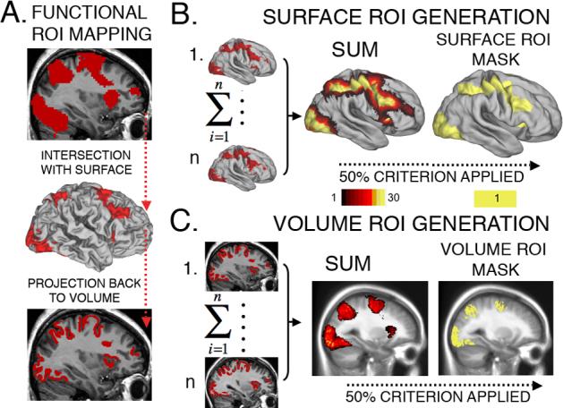
(A) Top panel: the functional ROI defined using conjunction analyses in 3D (all voxels that were active in both working memory domains across both patients and controls). Middle panel:group functional ROI mapped onto a subject's surface, thus limiting activation to the cortical ribbon. Bottom panel: cortical activation mapped back into the volume domain, thereby preserving only cortical signals. (B) After repeating this process for each subject's surface (left), the activation ROIs were summed (center), and regions above a threshold overlap (50%) were set to a value of 1 (right) to yield the final surface functional ROI mask. The mask shown is for controls; the mask for patients was very similar. (C) The individual cortical ROIs were mapped to volume representation (left), summed (middle), and regions above a threshold overlap (50%) were set to a value of 1 (right). This resulted in equivalently generated functional ROI masks for both surface and volume domains.
The surface ROI maps were then summed across subjects separately for the SCZ and CTRL groups to avoid confounds in location of activation (Fig. 4B, left). The final summation map is shown for CTRL group on the PALS-B12 average right fiducial surface in Fig. 4B (center). Surface nodes in which half or more of the subjects overlapped were used to define the surface mask for that group (Fig. 4B, right panel).
A similar analysis was done to generate a volume mask. Cortical volume ROIs for each individual (Fig. 4C, left) were summed across all subjects (Fig. 4C, middle), then thresholded at the 50% level to yield a corresponding volume mask (Fig. 4C, right). Because these functional ROIs were generated using a volume-driven analysis and then constrained using the cortical surface, this approach, as noted by Argall et al. (2006) should not be biased strongly towards either representation. Since the ROI was initially derived from a volume analysis, if anything it would have a slight bias towards the volume analysis.
This approach was similar to that used by Argall et al. (2006), except that they applied a constraint of approximately 30% overlap. Our use of a more stringent 50% overlap cutoff would tend to have a larger impact on ROI size for VBR vs SBR (owing to poorer registration) and would thus emphasize mainly peak responses in the VBR results. This should tend to increase the mean activation in VBR compared to SBR, but peaks should be unaffected.
The sulcal-based ROI generation involved the same five sulci used for the SAP and VAP analyses: the central, superior, frontal, inferior frontal, intraparietal, and calcarine sulci. We used the same overlap strategy outlined above for defining functional benchmark ROIs. This yielded unbiased sulcal ROIs that were independent of the peak fMRI signals.
The analogous approach was also carried out for group comparison maps (t-test of differences in working memory between patients and controls). For a complete description of between-group power analysis and results we refer the reader to online supplementary materials.
Results
We first present results for sulcal alignment precision, evaluated for different overlap stringency criteria and different cortical thickness values. The next section qualitatively illustrates fMRI power gains using SBR and spatial signal preservation using surface smoothing. The final section includes quantified power comparisons between VBR and SBR carried out using functional and anatomical ROI selection.
Cortical Alignment Precision
Figure 5 compares the precision with which a selected group of five sulci are aligned with one another using affine VBR and landmark-based SBR. In Fig. 5A, sulcal alignment precision values are similar for left (top row) and right (bottom row) hemispheres, with the best alignment for the CeS (far left) and the worst for the IFS (far right). The data were analyzed using repeated-measures ANOVA, with hemisphere (left, right), group (CTRL, SCZ), method (SBR, VBR) and sulcal identity (CeS, CaS, IPS, SFS, IFS) as factors. The results indicate that the difference between SBR and VBR was highly significant [main effect of method: F(1, 57)=1342, p<0.0001], with SBR alignment (gray, black) better than VBR alignment (light, dark green) for all 20 comparisons. There is a highly significant difference in alignment precision across various sulci [main effect of location F(4, 228)=441, p<0.0001], but no significant main effect of hemisphere [F(1, 57)=0.2, p<0.64]. Importantly, the benefits of SBR over VBR were significantly greater for patients with SCZ (light shading) than for controls (dark shading). This is apparent from the fact that the difference between SBR and VBR values was greater for SCZ (gray vs light green) than for controls (black vs dark green) for each sulcus in both hemispheres. Statistically, the ANOVA indicated a significant method by group interaction [F(1, 57)=49, p<0.0001]; the main effects of method for patients and controls separately were significant [F(1, 28)=735, p<0.0001 and F(1, 29)=606, p<0.0001 respectively]; the effect size of the main effect of method was greater in individuals with SCZ (d = 6.65) than controls (d = 5.42). The difference between SBR and VBR was confirmed for individual sulci using paired t-tests that compared SBR to VBR for each sulcus, analyzed separately by SCZ and CTRL groups and by hemisphere. Of the 20 comparisons, 19 showed SBR to have significantly better alignment than VBR, with 18 comparisons at or above p<0.001 levels, and one additional comparison (SFS for the CTRL on the right) significant at p<0.05.
Figure 5. Alignment precision quantification.
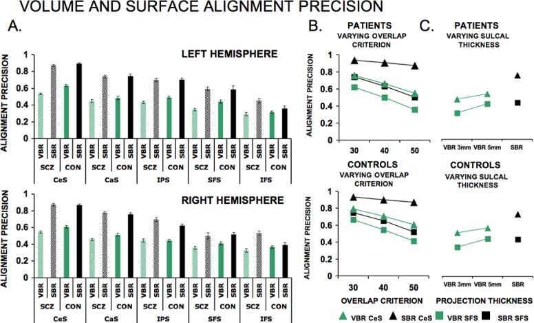
(A) Alignment precision results for left (top) and right (bottom) hemispheres. In each graph results are plotted in decreasing order of alignment precision for the five sulci. For each sulcus, results for both patient (shaded colors) and control (solid colors) groups are shown for both SBR (black) and VBR (green). (B) Results of decreasing overlap criterion for alignment precision metrics for SBR (black) and VBR (green) shown for patients (top) and controls (bottom) in the CeS (triangles) and SFS (squares). (C) Results of varying cortical thickness when projecting sulcal outlines to 3D domain shown for patients (top) and controls (bottom) for SBR (black) and VBR (green) in CeS (triangles) and SFS (squares).
To test whether the differences between SBR and VBR depended on the stringency criterion used to quantify alignment precision, we varied the stringency of the overlap criterion (see Methods, Metrics for Quantitative Comparison). As the overlap criterion becomes more lenient (smaller value), the overlap region increases in size, more sulcal territory across individuals should overlap, and the alignment index should increase. Besides the 50% overlap used for the main analysis, we tested values of 30% and 40% overlap for two sulci (CeS and SFS) that represent different degrees of alignment accuracy in both SBR and VBR. Figure 5B demonstrates that SBR (black points) outperformed VBR (green points) for all three overlap values tested for both the CeS (circles) and the SFS (squares). A repeated measures ANOVA model with group as a between subject factor (CTRL, SCZ) and criterion overlap (30%, 40%, 50%), sulcal identity (CeS, SFS) and alignment method (SBR, VBR) as within-subject factors indicated that the difference between SBR and VBR was highly significant [main effect of method, F(1, 57)=179, p<0.0001], more so for CeS than SFS [method by sulcus interaction, F(1, 57)=13, p<0.0001], more so for higher overlap criterion [2-way method by overlap criterion, F(2, 114)=24, p<0.0001], with a significant 3-way method by sulcus by overlap criterion interaction [F(2, 114)=10, p<0.0001]. The significance of the 3-way method by sulcus by overlap criterion interaction can be interpreted in terms of two lower order interactions that are both significant. After collapsing across both sulcal locations and both groups SBR outperforms VBR to a greater extent as the overlap criterion becomes more stringent. Similarly, collapsing across all three overlap criterions and both groups, SBR outperforms VBR to a greater extent for the CeS than for the SFS. The third order interaction also indicates that the increasingly greater benefit for SBR over VBR as the overlap criterion gets more stringent is greater for the CeS than the SFS.
Another concern was that the VBR analysis might have been at a disadvantage if the 3 mm thickness of the cortical ribbon in the volume domain underestimated the actual cortical thickness for the sulci being analyzed. We therefore used a ribbon thickness of 5 mm as well as 3 mm for the CeS and SFS (Fig. 5C) and applied this to the VBR analysis (but not the SBR, whose values are independent of thickness) A repeated measures ANOVA model with group as a between subject factor (CTRL, SCZ) and thickness (3 mm and 5 mm), sulcal landmark (CeS, SFS) and alignment method (SBR, VBR) as three within subject factors indicated a significant main effect of method [F(1, 58)=135, p<0.0001], a significant 2-way method by sulcus interaction [F(1, 58)=34, p<0.0001], a significant 2-way method by thickness interaction [F(1, 58)=2733, p<0.0001], and a significant 3-way method by sulcus by thickness interaction [F(1, 58)=186, p<0.0001]. As before, interpreting the 3-way method by sulcus by thickness interaction involves two lower order interactions that are both significant. Collapsing across sulcal locations and groups, SBR outperforms VBR to a greater extent as the thickness decreases; collapsing across thickness parameters and groups, SBR outperforms VBR to a greater extent for the CeS than the SFS. The third order interaction indicates that the increasingly greater benefit for SBR over VBR as the thickness parameter gets smaller is even greater for the CeS sulcus than the SFS. SBR substantially outperforms VBR for both cortical thickness values and both groups. For the SFS, SBR outperforms VBR for the cortical thickness of 3 mm, and the two measures are roughly equal for the 5 mm value.
Power Gains and Spatial Topography Preservation with SBR
Figure 6 shows functional maps that provide a qualitative illustration of the power gains in SBR using the IV (interpolated voxel) mapping method (top row) over VBR (bottom row) when no smoothing was applied to the data. All the maps shown were thresholded at T>3. The results for patients (left column) and controls (right column) are displayed on the very inflated PALS atlas surface. The dotted circles, centered on prefrontal and parietal regions robustly activated for working memory tasks, show substantially stronger activations for SBR, compared to VBR in these regions, particularly for the SCZ group. Similar results were seen for both working memory conditions across both hemispheres.
Figure 6. Statistical maps for SBR and VBR results.
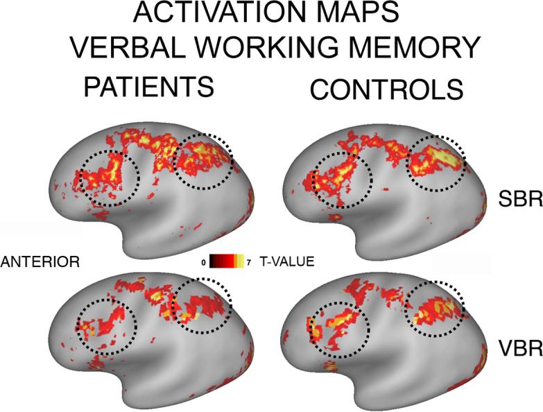
Activation pattern for verbal working memory task (thresholded at t>3; above-baseline activations only). Both volume and surface data were mapped to the PALS-B12 very inflated surface. Top and bottom panels: SBR and VBR results, respectively. Left and right panels: results for patients and controls, respectively. Black dotted circles indicate prefrontal and parietal regions where activations are stronger for SBR, especially in patients.
Figure 7A shows the results of smoothing the fMRI signal in 3D for a single individual. A small activation patch (yellow) discernible on the superior temporal gyrus (STG) when no smoothing was applied (black circle, left panel) disappeared when 9 mm Gaussian smoothing was applied (right panel). The same patch after mapping to the surface is shown on an inflated configuration (Fig. 7B) and in an expanded view of temporal cortex (Fig. 7C). In Figure 7C, the white circle outlines the peak signal on the STG (left panel), which persisted when the data were smoothed on the surface (middle panel), but disappeared after smoothing the signal in the volume domain (right panel). This patch is likely to be signal, not noise, as it was preserved across the entire length of the STG even at a high surface smoothing strength (∼12 mm FWHM). Furthermore, from inspection of individual subject data this was one of many examples that illustrate comparable signal loss using VBR.
Figure 7. Effect of 2D and 3D smoothing on spatial configuration of fMRI signal in a single subject.
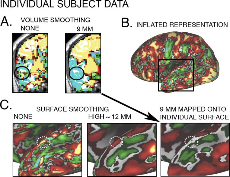
(A) Coronal slices of left hemisphere verbal working memory fMRI pattern before smoothing (left panel), with a signal (red, yellow voxels inside black circle) near the superior temporal gyrus (STG, white cortical ribbon outline) and after volume smoothing (right panel), with loss of STG activation patch (no red or yellow voxels inside black circle)(B) Same activation pattern as in (A) mapped to the individual left hemisphere using the IV method and displayed on a very inflated surface. Boxed region centered on the STG is expanded in (C). (C) Surface maps centered on STG (white circle) show activation visible before smoothing (left panel), and after surface smoothing(center panel; ∼12 mm FWHM Gaussian kernel), but not after volume smoothing (right panel; 9 mm Gaussian kernel).
To compare surface-based smoothing vs. volume-based smoothing applied to population-averaged data, Figure 8 shows the group T-statistic results of word working memory activation for the left hemisphere (in this case shown only for patients) visualized on the PALS-B12 surface. Figure 8A shows an inflated cortical surface model with the occipital lobe highlighted and shown in a zoomed representation in panels B-E. Figure 8B shows the population-average task activation after SBR with no smoothing applied. The black circles are centered on two peaks of activation. Figure 8C shows that with the data smoothed on the surface [strength=0.6, iterations=30, approximate FWHM Gaussian blur of 12 mm] the signal-to-noise is substantially enhanced; yet the two peaks remain distinct. Figure 8D shows the results of volume analysis visualized on the surface with no smoothing applied. The same two peaks are present but not as pronounced. Figure 8E shows the results of 9 mm Gaussian smoothing applied in the volume. The signal-to noise is much more enhanced, but the two peaks are now completely merged. In this instance, the improved spatial resolution occurs in a region associated with modest shape variability in terms of the 3-D variability and sulcal depth variability after mapping a population of subjects to the PALS-B12 atlas (Fig. 6 in Van Essen, 2005).
Figure 8. Improved spatial resolution for surface smoothing vs volume smoothing.

Verbal working memory activations are shown (t>3) for the left hemisphere. (A) Inflated cortical map with rectangular selection centered on the primary visual cortex. (B) SBR data with no smoothing applied. The two activation peaks are highlighted with black circles. (C) SBR data with high smoothing strength applied (∼12 mm FWHM Gaussian kernel). The peak separation inside the black outlines is still preserved. (D) VBR data with no smoothing applied. The peak separation inside the black outlines is still preserved, although clearly attenuated. (E) VBR data with a 9 mm Gaussian kernel applied. The peak separation inside the black outlines is lost and there is spreading of the signal beyond the level observed when even stronger smoothing was applied on the surface. (F-J) The same pattern of results is shown for a selection centered on the left parietal cortex shown in a flattened representation.
Figure 8F-J shows another example of a similar loss in spatial resolution for 3D smoothing compared to 2D smoothing with signal in the parietal cortex. In this instance, the cortical region involved is associated with a high degree of shape variability (Van Essen 2005), indicating that the benefits of SBR in improving spatial resolution apply widely throughout the cortex and well away from the landmarks used to constrain registration.
Functional ROI-based power analysis
We compared SBR and VBR statistical power profiles using functional benchmark ROIs generated from an analysis across both tasks (face and word working memory) and groups (see methods and Fig. 4 for details). Figure 9A shows that for unsmoothed data, SBR (black symbols) generally outperforms VBR (green symbols) across all domains of comparison in both patients (circles) and controls (bars). We tested for the maximum t-value (left), mean t-value (right), and median t-value (see Supplementary Material) for nodes (SBR) or voxels (VBR) within the functional benchmark ROI. In 23 of 24 comparisons for the data that received no volume smoothing and were mapped using the IV method, black symbols lie above the green symbols. Moreover, the difference between SBR (black) and VBR (green) was generally larger for SCZ (circles) than for controls (bars). To test the statistical significance of these differences, we conducted three separate analyses with different criteria (SBR-VBR t-statistic difference exceeded 0, 0.25 and 0.5 in absolute value). The 0.25 criterion was maximally sensitive to the differences and is reported here, but the results were similar for the other two criteria (see Supplementary Material). The analysis included 3 statistical parameters (i.e. max, mean, median), 4 conditions of comparison (i.e. face and word working memory each on the right and left), and two groups (i.e. CTRL and SCZ) for a total of 24 possible comparison points for each smoothing condition. For the unsmoothed data (Fig. 9A) the SBR proportion was higher than VBR (proportion significantly higher than chance, p<0.0001, by binomial test). Furthermore, the power advantage for SCZ versus CTRL group exceeded chance [Z=2.0, p<0.03 by Z distribution test]. Figure 9 also shows a subset of the analyses (non-verbal working memory on the right hemisphere) conducted using the EV mapping technique (Fig. 9, far right category on the abscissa), with a slight advantage evident for SBR. Compared to the IV method, the mean and median values were lower for SBR when the EV method was applied to the unsmoothed data (see Discussion).
Figure 9. Power comparison results using the functional ROI.

(A) Unsmoothed data are shown two parameters (max and mean) for both hemispheres and both working memory conditions. Green and black data points show VBR and SBR results respectively with patient data shown in circles and control data are shown in horizontal bars. Overall, there is an elevated power profile for SBR. (B) Analogous results are shown with 9 mm Gaussian kernel smoothing in 3D, then analyzed in surface and volume. The far right category on the abscissa shows data mapped using the EV method for non-verbal working memory on the right hemisphere.
When the data were smoothed by a 9 mm Gaussian kernel in volume space (Fig. 9B) the t-values increased markedly, reflecting the improved SNR, and two methods were roughly comparable (proportion between SBR and VBR not significantly different than chance, p<0.1, by binomial test). This is not surprising because spatial smoothing in the volume necessarily erodes the advantage of SBR (see Discussion).
Anatomical ROI-based power analysis
Using an approach similar to that of the preceding section, we carried out power analyses across five anatomical ROIs for both face working memory and word working memory on both hemispheres. Figure 10 shows results for face working memory on the right hemisphere (see Supplementary Material for other comparisons) applied to non-smoothed data (Fig. 10A) and to volume-smoothed data (Fig. 10B). We used the same three criteria applied to the functional ROI (here we report absolute difference of 0.25 or greater) to test for a difference in power between SBR and VBR for the anatomical ROIs. Again, we used statistical parameters of max (left), mean (right) and median (see Supplementary Material) and there were 4 conditions of comparison (i.e. face and word working memory on the right, face and word working memory on the left ) and two groups (i.e. CTRL and SCZ) and 5 possible anatomical locations (i.e. CeS, CaS, IPS, SFS, & IFS) resulting in a total of 120 points of comparison for SBR and VBR for each smoothing condition.
Figure 10. Power comparison using anatomical ROIs (right hemisphere, face working memory).

(A) Data are shown across all five anatomical ROIs. Green (B) Analogous results are shown for smoothed data.
In brief, the SBR advantages observed in functional ROI-based analyses were also evident in the anatomical ROI analyses. Overall, for the unsmoothed data (subset shown in Fig. 10A) SBR power profiles were higher than VBR (proportion for SBR significantly higher than chance, p<0.0001, by binomial test). However, unlike the functional ROI, there was no differential advantage for patients versus controls [Z=0.65, p<0.3 by Z distribution test]. When the data were smoothed by a 9 mm Gaussian kernel in volume space (Fig. 10B) SBR still showed some advantage over VBR, but as expected the magnitude of this advantage was less than in the unsmoothed data. However, when collapsing across possible points of comparison in the smoothed data, SBR power profiles were higher than VBR (proportion for SBR significantly higher than chance, p<0.0001, by binomial test). Additionally, when the data were smoothed, the power advantage was significantly greater for patients [Z=1.84, p<0.04 by Z distribution test].
As with the functional ROIs, we made a subset of comparisons (face working memory on the right hemisphere) using the EV mapping algorithm applied to unsmoothed data (Fig. 11A) and volume-smoothed data (Fig. 11B). As before, we used a criterion (absolute difference of 0.25 or greater) to test for a power difference between SBR and VBR (the results of other criteria are reported in Supplementary Material). There were 3 statistical parameters (i.e. max, mean, median), one condition of comparison (i.e. face working memory on the right), two groups (i.e. CTRL and SCZ), and 5 possible anatomical locations (i.e. CeS, CaS, IPS, SFS, & IFS). Overall, the results showed a significant difference between VBR and SBR, (proportion for SBR significantly higher than chance, p<0.05, by binomial test).
Figure 11. Power comparison using anatomical ROIs (right hemisphere, face working memory) enclosing voxel mapping.

The data in this figure were mapped onto individual surface models using the enclosing voxel technique and follow the same outline as figure 10.
Analogous comparisons of power for between-group differences were carried out and are presented in online Supplementary Material.
Discussion
Cortical Alignment Precision
We confirmed previous findings showing improved cortical alignment with landmark-based SBR compared to affine VBR in healthy control subjects (Van Essen, 2005; Van Essen and Dierker, 2007) and extended the findings by demonstrating even greater alignment improvement when using SBR in patients with SCZ. To our knowledge this is the first study that compared SBR and VBR for alignment of cortical sulci in a patient population. These results indicate that SBR can reduce the impact of anatomical anomalies on registration quality compared to affine VBR.
Estimates of alignment precision in VBR depend on the value used for cortical ribbon thickness. We addressed this issue by comparing an average cortical thickness projection of 3 mm as well as an exaggerated thickness of 5 mm. In both cases SBR produced significantly better alignment of the CeS location, which is not surprising since this sulcus provides one of the registration landmarks. In the more variable SFS, SBR outperformed VBR at 3 mm, though the two methods did not differ significantly at the exaggerated 5 mm thickness. Altogether, this analysis suggests that SBR yields better alignment than VBR but that the magnitude of the benefit varies regionally.
A separate issue was the choice of overlap criterion when calculating alignment precision metrics. The better the alignment algorithm, the more stringent the criterion can be and still produce good alignment precision metrics (see Methods). This can in turn make the observed differences between alignment methods appear even greater. As expected, the differences between methods were decreased when the overlap was reduced from 50% to 30%. However, even at the liberal 30% overlap, SBR yielded better alignment than VBR.
Spatial Preservation of Signal
Consistent with previous simulation studies (Hagler et al., 2006; Jo et al., 2007), we demonstrated that the application of spatial smoothing in 2D improves signal-to-noise while preserving the location of activation peaks more accurately than does smoothing in 3D. As noted in the Introduction, a fundamental issue is that Gaussian smoothing in 3D does not take into account local cortical folding patterns. Although 3D smoothing remains the preferred strategy for subcortical structures, the present study provides further evidence that surface-based analyses are advantageous for cortical signals. In general, SBR should yield gains but not losses in terms of spatial localization and signal power as long as the surface reconstructions are sufficiently high in quality and the fMRI data are well aligned to the structural data. Gains in spatial localization are also attainable using anisotropic volume smoothing that takes into account cortical surface orientation in a canonical brain (Kiebel and Friston, 2002). Given the high degree of individual variability, greater benefits would presumably accrue from anisotropic volume smoothing constrained by cortical surface orientation in individual subjects.
If fMRI voxel size approaches or exceeds cortical thickness, voxels centered on sulcal gray matter will typically include a mixture of signals from opposite banks of the sulcus. Hence, coarse fMRI sampling (and also poor alignment between functional and structural data) will necessarily erode the benefits attainable using structural data. Given that much of the fMRI data in the present study was acquired at 7 mm resolution along one dimension, the benefits we demonstrated for SBR are likely to underestimate the maximum that is attainable. It is important to repeat and extend these comparisons using higher resolution fMRI data.
Statistical Power in SBR and VBR
For a fair comparison of statistical power between SBR and VBR, it is important to avoid biases that would unduly benefit or penalize either approach. The ROI within which power is analyzed represents one potential source of bias, because SBR analyses are concentrated in cortical gray matter, whereas in VBR each voxel in the population average is typically derived from a mixture of tissue types (gray matter, white matter, CSF). We used the approach developed by Argall et al. (2006) in which minimally biased ‘benchmark’ anatomical or functional ROIs were restricted to the average thickness cortical ribbon (3 mm, see Methods).
For the main analyses we used the interpolated voxel (IV) mapping algorithm, which combines evidence from all fMRI voxels that intersect cortical gray matter associated with any given surface node (i.e., along the radial axis above and below the node). For example, if one voxel intersects gray matter in superficial layers and another intersects in deep layers, the IV method assigns a value for a node at the cortical mid-thickness that represents balanced contributions from both voxels. One or both of these voxels may include partial volume contributions from noncortical regions (CSF, subcortical white matter) or from gray matter on an opposing sulcal bank, but this is an unavoidable consequence of fMRI voxel size.
The results largely confirmed our expectation that statistical power would be enhanced in SBR using the IV method. The larger power gain for the SCZ group tested using the functional benchmark ROI suggests that SBR can be particularly advantageous for analyses of fMRI activation patterns in disease conditions. The gain was less pronounced using anatomical ROI approach, presumably reflecting widespread sampling of cortical territories in the anatomical ROIs that were not centered at the peaks of activation in the working memory task. Because activation patterns in the SCZ group may be more heterogeneous (Manoach et al, 2000; see Manoach, 2003 for review), anatomical ROIs might not overlap as well with the more variable activation pattern in the SCZ group.
The outcome was somewhat different using the enclosing voxel (EV) mapping algorithm, in which each surface node is assigned the value of the fMRI voxel in which it resides, regardless of whether the node is close to the center or near the margins of the voxel. Using the EV method, there was a trend towards superior performance for SBR vs. VBR with the functional ROI method, but the difference was not significant. However, with the more spatially unbiased and widespread anatomical ROI method there was an overall significant advantage for SBR. The difference between EV and IV mapping methods can be interpreted in two ways. One argument is that the EV method is conceptually inferior to the IV method owing to its failure to sample all of the voxels that intersect cortical gray matter at a given location. The other is that the IV method by its nature includes some degree of spatial smoothing, insofar as it provides a weighted average of signal from multiple voxels. (The degree of smoothing is ∼3 mm on average, as documented in Supplementary Material.) This issue needs to be addressed more systematically, but such analyses should be carried out using both simulated data (circumventing confounds related to alignment of functional and structural volumes) and from fMRI data acquired at uniformly high spatial resolution for all subjects (functional data in this study were resampled to 3 mm cubic voxels from an originally coarser resolution as outlined in methods).
Importantly, although the power benefits for SBR versus VBR were not evident when the data received 9 mm volumetric smoothing (see tables 1-3 in Supplementary Material), VBR results were accompanied by a costly loss of spatial resolution that was preserved when data were smoothed in a 2D domain.
Further, as was previously mentioned, we carried out power comparison between-group differences in WM, which are presented in Supplementary Material. The power differences between SBR and VBR for the between-group comparison were attenuated compared to the within group results , with no consistent advantage for either method. This finding is perhaps not surprising given the added power benefit for patients in the within-group SBR analysis, which may have actually served to reduce differences between patients and controls.
Alignment Algorithm
The degree to which SBR provides alignment and fMRI power benefits over VBR will obviously depend upon the particular choices of the SBR and VBR algorithms. Landmark-based registration to the PALS-B12 atlas, as used in the present study differs in important ways from alternative SBR methods such as that used in FreeSurfer. FreeSurfer uses an energy-minimization approach to maximize the alignment between the ‘average convexity’ (similar but not identical to our sulcal depth measure) and a population-average spherical atlas generated from a different group of subjects and a different atlas-generation process (Fischl et al., 1999b). Direct comparisons between different SBR algorithms (e.g. Desai et al., 2005; Argall et al., 2006) that objectively assess the advantages and limitations of each will help investigators choose which approach best fits their specific research questions. There is a similar need to evaluate the alignment quality achieved by nonlinear VBR, both low and high-dimensional VBR (e.g., Ashburner & Friston, 1998; Schormann et al., 1998; Woods et al., 1998-II; Miller et al., 2005) and anatomically constrained VBR (Kiebel and Friston, 2002) in comparison to SBR techniques.
Conclusion
The present study demonstrates that landmark-based SBR to the PALS-B12 atlas is superior to affine VBR for aligning cortical sulci. Furthermore, we demonstrated that this improvement extends to analyses of cortical fMRI signals, resulting in improved power profiles for data that received little or no smoothing. Practically, this suggests that with improved alignment and power, a less aggressive smoothing kernel is required when using the PALS SBR framework. This in turn allows improved spatial resolution over that obtained with VBR for fMRI studies of human cortical function. Lastly, we showed that both of these advantages are even greater for patients with SCZ.
Supplementary Material
Acknowledgements
We thank S. Petersen and M. Strube for helpful comments and analysis suggestions. Supported by NIMH grant MH06603101 (DMB) and NIMH grant MH071616 (JGC and DMB), and NIH Grant R01-MH-60974, funded by the National Institute of Mental Health, the National Institute for Biomedical Imaging and Bioengineering, and the National Science Foundation (DCVE and DLD).
Footnotes
Publisher's Disclaimer: This is a PDF file of an unedited manuscript that has been accepted for publication. As a service to our customers we are providing this early version of the manuscript. The manuscript will undergo copyediting, typesetting, and review of the resulting proof before it is published in its final citable form. Please note that during the production process errors may be discovered which could affect the content, and all legal disclaimers that apply to the journal pertain.
Contributor Information
Alan Anticevic, Department of Psychology, Washington University in St. Louis.
Donna L. Dierker, Department of Anatomy and Neurobiology, Washington University in St. Louis
Sarah K. Gillespie, Department of Psychiatry, Washington University in St. Louis
Grega Repovs, Department of Psychology, Washington University in St. Louis.
John G. Csernansky, Department of Psychiatry, Washington University in St. Louis
David C. Van Essen, Department of Anatomy and Neurobiology, Washington University in St. Louis
Deanna M. Barch, Department of Psychology, Washington University in St. Louis
References
- Acton PD, Friston KJ. Statistical parametric mapping in functional neuroimaging: beyond PET and fMRI activation studies. Eur. J. Nucl. Med. 1998;25:663–667. [PubMed] [Google Scholar]
- Andrade A, Kherif F, Mangin JF, Worsley KJ, Paradis AL, Simon O, et al. Detection of fmri activation using cortical surface mapping. Human brain mapping. 2001;12(2):79. doi: 10.1002/1097-0193(200102)12:2<79::AID-HBM1005>3.0.CO;2-I. [DOI] [PMC free article] [PubMed] [Google Scholar]
- Argall BD, Saad ZS, Beauchamp MS. Simplified intersubject averaging on the cortical surface using suma. Human brain mapping. 2006;27(1):14. doi: 10.1002/hbm.20158. [DOI] [PMC free article] [PubMed] [Google Scholar]
- Ashburner J, K.J. Friston KJ. High-Dimensional Nonlinear Image Registration. NeuroImage. 1998;7(4):S737. doi: 10.1006/nimg.1999.0437. 1998. [DOI] [PubMed] [Google Scholar]
- Baddeley AD. Working memory. Oxford University Press; New York: 1986. [Google Scholar]
- Barch DM, Carter CS, Braver TS, McDonald A, Sabb FW, Noll DC, et al. Selective deficits in prefrontal cortex regions in medication naive schizophrenia patients. Archives of General Psychiatry. 2001;50:280–288. doi: 10.1001/archpsyc.58.3.280. [DOI] [PubMed] [Google Scholar]
- Barch DM, Csernansky J, Conturo T, Snyder AZ, Ollinger J. Working and long-term memory deficits in schizophrenia. Is there a common underlying prefrontal mechanism? Journal of Abnormal Psychology. 2002;111:478–494. doi: 10.1037//0021-843x.111.3.478. [DOI] [PubMed] [Google Scholar]
- Braver TS, Barch DM, Kelley WM, Buckner RL, Cohen NJ, Meizin FM, et al. Direct comparison of prefrontal cortex regions engaged by working and long-term memory tasks. NeuroImage. 2001;14:48–59. doi: 10.1006/nimg.2001.0791. [DOI] [PubMed] [Google Scholar]
- Cohen JD, MacWhinney B, Flatt MR, Provost J. Psyscope: A new graphic interactive environment for designing psychology experiments. Behavioral Research Methods, Instruments & Computers. 1993;25(2):257–271. [Google Scholar]
- D'Esposito M, Detre JA, Alsop DC, Shin RK, Atlas S, Grossman M. The neural basis of the central executive system of working memory. Nature. 1995;378(November 16):279–281. doi: 10.1038/378279a0. [DOI] [PubMed] [Google Scholar]
- Dale AM, Sereno MI. improved localization of cortical activity by combining EEG and MEG with MRI cortical surface reconstruction — a linear approach. J Cogn Neurosci. 1993;5:162–176. doi: 10.1162/jocn.1993.5.2.162. [DOI] [PubMed] [Google Scholar]
- Dale AM, Fischl B, Sereno MI. Cortical surface-based analysis. I. Segmentation and surface reconstruction. NeuroImage. 1999;9(2):179. doi: 10.1006/nimg.1998.0395. [DOI] [PubMed] [Google Scholar]
- Desai R, Liebenthal E, Possing ET, Waldron E, Binder JR. Volumetric vs. surface-based alignment for localization of auditory cortex activation. Neuroimage. 2005;26:1019–29. doi: 10.1016/j.neuroimage.2005.03.024. [DOI] [PubMed] [Google Scholar]
- Fischl B, Sereno MI, Tootell RB, Dale AM. High-resolution intersubject averaging and a coordinate system for the cortical surface. Human brain mapping. 1999;8(4):272. doi: 10.1002/(SICI)1097-0193(1999)8:4<272::AID-HBM10>3.0.CO;2-4. [DOI] [PMC free article] [PubMed] [Google Scholar]
- Fischl B, Dale AM. Measuring the thickness of the human cerebral cortex from magnetic resonance images. Proceedings of the National Academy of Sciences of the United States of America. 2000;97(20):11050. doi: 10.1073/pnas.200033797. [DOI] [PMC free article] [PubMed] [Google Scholar]
- Fischl B, Sereno MI, Dale AM. Cortical surface-based analysis. II. Inflation, flattening, and a surface-based coordinate system. Neuroimage. 1999a;9:195–207. doi: 10.1006/nimg.1998.0396. [DOI] [PubMed] [Google Scholar]
- Fischl B, Sereno MI, Tootell RB, Dale AM. High-resolution intersubject averaging and a coordinate system for the cortical surface. Human Brain Mapping. 1999;8:272–284. doi: 10.1002/(SICI)1097-0193(1999)8:4<272::AID-HBM10>3.0.CO;2-4. [DOI] [PMC free article] [PubMed] [Google Scholar]
- Friston KJ, Holmes AP, Poline JB, Grasby PJ, Williams SC, Frackowiak RS, et al. Analysis of fmri time-series revisited. NeuroImage. 1995;2(1):45. doi: 10.1006/nimg.1995.1007. [DOI] [PubMed] [Google Scholar]
- Goebel R. BrainVoyager: a program for analyzing and visualizing functional and structural magnetic resonance data sets. Neuroimage. 1996;3:S604. [Google Scholar]
- Goebel R. BrainVoyager 2.0: from 2D to 3D fMRI analysis visualization. Neuroimage. 1997;5:S635. [Google Scholar]
- Goldman-Rakic PS. Working memory dysfunction in schizophrenia. Journal of neuropsychiatry. 1994;6(4):348–357. doi: 10.1176/jnp.6.4.348. [DOI] [PubMed] [Google Scholar]
- Gray JR, Braver TS, Raichle ME. Integration of emotion and cognition in the lateral prefrontal cortex. Proceedings of the National Academy of Sciences USA. 2002;99:4115–4120. doi: 10.1073/pnas.062381899. [DOI] [PMC free article] [PubMed] [Google Scholar]
- Hagler DJ, Jr., Saygin AP, Sereno MI. Smoothing and cluster thresholding for cortical surface-based group analysis of fMRI data. Neuroimage. 2006;33:1093–1103. doi: 10.1016/j.neuroimage.2006.07.036. [DOI] [PMC free article] [PubMed] [Google Scholar]
- Jenkinson M, Smith SM. A global optimisation method for robust affine registration of brain images. Medical Image Analysis. 2001;5(2):143–156. doi: 10.1016/s1361-8415(01)00036-6. [DOI] [PubMed] [Google Scholar]
- Jenkinson M, Bannister PR, Brady JM, Smith SM. Improved optimisation for the robust and accurate linear registration and motion correction of brain images. NeuroImage. 2002;17(2):825–841. doi: 10.1016/s1053-8119(02)91132-8. [DOI] [PubMed] [Google Scholar]
- Jo HJ, Lee J-M, Kim J-H, Shin Y-W, Kim I-Y, Kwon JS, et al. Spatial accuracy of fmri activation influenced by volume- and surface-based spatial smoothing techniques. NeuroImage. 2007;34(2):550. doi: 10.1016/j.neuroimage.2006.09.047. [DOI] [PubMed] [Google Scholar]
- Kelley WM, Miezin FM, McDermott KB, Buckner RL, Raichle ME, Cohen NJ, et al. Hemispheric specialization in human dorsal frontal cortex and medial temporal lobe for verbal and non-verbal memory encoding. Neuron. 1998;20:927–936. doi: 10.1016/s0896-6273(00)80474-2. [DOI] [PubMed] [Google Scholar]
- Kiebel S, Friston KJ. Anatomically Informed Basis Functions in Multisubject Studies. Human Brain Mapping. 2002;16:36–46. doi: 10.1002/hbm.10021. [DOI] [PMC free article] [PubMed] [Google Scholar]
- Logan JM, Sanders AL, Snyder AZ, Morris JC, Buckner RL. Under-recruitment and nonselective recruitment: Dissociable neural mechanisms associated with aging. Neuron. 2002;33:827–840. doi: 10.1016/s0896-6273(02)00612-8. [DOI] [PubMed] [Google Scholar]
- Manoach DS, Gollub RL, Benson ES, Searl MM, Goff DC, Halpern E, Saper CB, Rauch SL. Schizophrenic subjects show aberrant fMRI activation of dorsolateral prefrontal cortex and basal ganglia during working memory performance. Biological Psychiatry. 2000;48:99–109. doi: 10.1016/s0006-3223(00)00227-4. [DOI] [PubMed] [Google Scholar]
- Manoach DS. Prefrontal cortex dysfunction during working memory performance in schizophrenia: reconciling discrepant findings. Schizophrenia Research. 2003;60:285–298. doi: 10.1016/s0920-9964(02)00294-3. [DOI] [PubMed] [Google Scholar]
- Miller MI, Beg MF, Ceritoglu C, Stark C. Increasing the power of functional maps of the medial temporal lobe by using large deformation diffeomorphic metric mapping. Proc Natl Acad Sci. 2005;102(27):9685–90. doi: 10.1073/pnas.0503892102. [DOI] [PMC free article] [PubMed] [Google Scholar]
- Nichols TE, Holmes AP. Nonparametric permutation tests for functional neuroimging: A primer with examples. Human Brain Mapping. 2001;15:1–25. doi: 10.1002/hbm.1058. [DOI] [PMC free article] [PubMed] [Google Scholar]
- Ojemann J, Akbudak E, Snyder A, McKinstry R, Raichle M, Conturo T. Anatomic localization and quantitative analysis of gradient refocused echo-planar fmri susceptibility artifacts. Neuroimage. 1997;6:156–167. doi: 10.1006/nimg.1997.0289. [DOI] [PubMed] [Google Scholar]
- Oldfield RC. The assessment and analysis of handedness: The edinburgh inventory. Neuropsychologia. 1971;9(1):97–113. doi: 10.1016/0028-3932(71)90067-4. [DOI] [PubMed] [Google Scholar]
- Ono M, Kubik S, Abernathey CD. Attas of the cerebral sulci. George Thieme Verlag; New York: 1990. [Google Scholar]
- Pitman EJG. A note on normal correlation. Biometrika. 1939;31:9–12. [Google Scholar]
- Schormann T, Zilles K. Three-dimensional linear and nonlinear transformations: an integration of light microscopical and MRI data. Human Brain Mapping. 1998;6:339–347. doi: 10.1002/(SICI)1097-0193(1998)6:5/6<339::AID-HBM3>3.0.CO;2-Q. [DOI] [PMC free article] [PubMed] [Google Scholar]
- Shenton ME, Dickey CC, Frumin M, McCarley RW. A review of mri findings in schizophrenia. Schizophrenia Research. 2001;49:1–52. doi: 10.1016/s0920-9964(01)00163-3. [DOI] [PMC free article] [PubMed] [Google Scholar]
- Talairach J, Tournoux P. Co-planar stereotaxic atlas of the human brain. Thieme; New York: 1988. [Google Scholar]
- Van Essen DC, Drury HA, Dickson J, Harwell J, Hanlon D, Anderson CH. An integrated software suite for surface-based analyses of cerebral cortex. Journal of the American Medical Informatics Association: JAMIA. 2001;8(5):443. doi: 10.1136/jamia.2001.0080443. [DOI] [PMC free article] [PubMed] [Google Scholar]
- Van Essen DC. A population-average, landmark- and surface-based (PALS-B12) atlas of human cerebral cortex. NeuroImage. 2005;28:635–662. doi: 10.1016/j.neuroimage.2005.06.058. [DOI] [PubMed] [Google Scholar]
- Van Essen DC, Dierker D. Surface-based and probabilistic atlases of primate cerebral cortex. Neuron. 2007;56:209–225. doi: 10.1016/j.neuron.2007.10.015. [DOI] [PubMed] [Google Scholar]
- Van Snellenberg JX, Torres IJ, Thornton AE. Functional Neuroimaging of Working Memory in Schizophrenia: Task Performance as a Moderating Variable. Neuropsychology. 2006;20:497–510. doi: 10.1037/0894-4105.20.5.497. [DOI] [PubMed] [Google Scholar]
- Woods RP, Grafton ST, Holmes CJ, Cherry SR, Mazziotta JC. Automated image registration: I. General methods and intrasubject, intramodality validation. Journal of Computer Assisted Tomography. 1998;22(1):139–152. doi: 10.1097/00004728-199801000-00027. [DOI] [PubMed] [Google Scholar]
- Woods RP, Grafton ST, Watson JDG, Sicotte NL, Mazziotta JC. Automated image registration: II. Intersubject validation of linear and nonlinear models. Journal of Computer Assisted Tomography. 1998;22(1):153–165. doi: 10.1097/00004728-199801000-00028. [DOI] [PubMed] [Google Scholar]
- Worsley KJ, Friston KJ. Analysis of fmri time-series revisited - again. Neuroimage. 1995;2:173–181. doi: 10.1006/nimg.1995.1023. [DOI] [PubMed] [Google Scholar]
Associated Data
This section collects any data citations, data availability statements, or supplementary materials included in this article.