Computer-Assisted Segmentation of White Matter Lesions in 3D MR images, Using Support Vector Machine

Abstract

Brain lesions, especially White Matter Lesions (WMLs), are associated with cardiac and vascular disease, but also with normal aging. Quantitative analysis of WML in large clinical trials is becoming more and more important. In this paper, we present a computer-assisted WML segmentation method, based on local features extracted from multi-parametric Magnetic Resonance Imaging (MRI) sequences, i.e. T1-weighted (T1-w), T2-weighted (T2-w), proton density-weighted (PD), and fluid attenuation inversion recovery (FLAIR) MR scans. A Support Vector Machine (SVM) classifier is first trained on expert-defined WML’s, and is then used to classify new scans. Subsequent post-processing analysis further reduces false positives by utilizing anatomical knowledge and measures of distance from the training set. Cross-validation on a population of 45 patients from 3 different imaging sites with WMLs of varying sizes, shapes and locations tests the robustness and accuracy of the proposed segmentation method, compared to the manual segmentation results from two experienced neuroradiologists.

INTRODUCTION

Cerebrovascular Disease (CVD) in elderly individuals is very important. In particular, CVD increases the likelihood of clinical dementia [1–4] even in the absence of clinical stroke [5], albeit the literature is somewhat inconclusive as to whether CVD has simply an additive role to Alzheimer’s Disease (AD) or there are interactions between the two. Approximately one third of patients that meet clinical and pathological diagnostic criteria for AD have some degree of vascular pathology [6, 7]. The impact of CVD on Mild Cognitive Impairment (MCI)—where the etiology of the cognitive deficit is generally less clear—is likely to be even greater. Therefore, in order to identify biological markers specific to the AD process, it is critical to also identify the extent of concurrent CVD related brain injury that is often clinically silent [8–11], since at the very least, CVD increases the likelihood of clinical presentation of dementia, for the same level of AD-related pathology.

Population studies, such as the Cardiovascular Health Study (CHS) or the Rotterdam Scan Study (RSS), have shown that brain lesions, especially WMLs, are associated with age, clinically silent stroke, higher systolic blood pressure, lower forced expiratory volume in 1 s, hypertension, atrial fibrillation, carotid and peripheral arterioscleroses, impaired cognition and depression [12–14]. Furthermore, it has been shown that stroke patients with a large WML load have an increased risk of hemorrhagic transformation, higher preoperative risk of a disabling or fatal stroke during endarterectomy or intercerebral hemorrhage during anticoagulation therapy [15]. The increased interest in brain lesion research may improve diagnosis and prognosis possibilities for patients with cardiovascular symptoms.

The relationship between Diabetes Mellitus (DM) and cognitive impairment, as well as with increased risk for dementia, has been documented by several clinical studies [16–18]. This relationship is mediated by brain pathology including cerebral infarcts, leukoareosis, and tissue atrophy [19–24]. Precise measurement of such pathology from MRI, and more importantly measurement of evolution of pathology over time, is very important for disease monitoring and evaluation of treatments for DM, such as controlling blood pressure and glycemia. All of these previous studies have employed subjective evaluation of brain lesions, such as the scale of [12] which examined the relationship between periventricular and subcortical WMLs and cognitive functioning in 1,077 elderly subjects randomly sampled from the general population, and are hampered by variations in the anatomical definition of brain abnormalities. Therefore, such methods of evaluation of brain abnormality in DM are not easily reproducible, qualitative, and nearly impossible to use without paired reading and high level of Quality Control (QC) in large multi-site studies and in longitudinal evaluations that might span over several years [25]. There is an increasing need for development of highly automated, validated, and reproducible computer-based image analysis tools, especially in large-scale longitudinal studies evaluating brain pathology in DM.

Since brain lesion patterns are very heterogeneous, ranging from punctuate lesions in the deep white matter to large confluent periventricular lesions, the scoring of such lesions is complicated. Moreoevr, it has been shown that different visual rating scales lead to inconsistencies among studies [26]. Commonly used ordinal brain lesion scoring methods, such as used in the CHS [27] or the RSS [12, 28], offer semi-quantitative information on the prevalence of such lesions. Exact spatial information is useful since it has been suggested that specific lesion patterns are associated with specific symptoms [29, 30]. Moreover, for longitudinal studies aiming to capture relatively small changes in brain lesion patterns, accurate information of lesion volume and location is essential. Expert-based delineation of brain lesions is known to be difficult to reproduce across raters, or even within the same rater, which makes it problematic and that combination of readings from independent reader may be necessary in a longitudinal study.

The use of an automated segmentation method that detects brain lesions with a high sensitivity and specificity could be advantageous. Most of the successful methods in the literature have been developed for the detection of Multiple Sclerosis (MS) lesions [31–46]. In early approaches when multi-modality images are not easily available, features describing normal tissue statistics (either intensity property alone or both intensity and spatial properties) are usually extracted from available modality and then combined with various classifiers, such as: minimum distance classifier, Bayesian classifier, decision tree, etc., for MS lesion segmentation purpose. In [31], Kamber et al built a voxel-wise probability normal tissue (GM-Grey Matter, WM-White Matter, VN-Ventricle) distribution model in Talairach space and then use decision tree to discriminate MS lesion tissue from normal tissue based on entropy minimization. A similar approach was pursued in [46], where spatial statistics of normal brain tissues were first determined from a training set, and deviations from normal variation were flagged as lesions. In [33], major brain tissues (WM, GM and CSF-CerebroSpinal Fluid) were modeled as fuzzy connected regions; potential MS lesions are regarded as isolated islands and were further refined by human judgment.

Most current imaging studies offer the potential to combine multi-parametric MR images, i.e. images obtained via different MR protocols. The advantage of integrating information from multiple sequences is that it can reduce the uncertainty and increase the accuracy of the segmentation. One can categorize most state of art lesion segmentation algorithms in two main categories: supervised voxel-wise classification and unsupervised clustering. In [37], Leemput et al proposed an unsupervised WML segmentation model via setting up a multivariate Gaussian model to describe normal tissue signal distribution, and using it to detect MS lesions as outliers. In supervised methods, a set of images in which the desired segmentation is known (expert manual delineation) is used as a training set to build and fine-tune the segmentation algorithm [35, 44]. In [41], based on the well-known medical image processing system – INSECT, Zijdenbos et al proposed a supervised MS lesion segmentation method using multi-spectral (T1-w, T2-w, PD) intensity signal and spatial prior as features and Artificial Neural Network (ANN) for classification purpose. The method was developed in the context of a phase III clinical trial and results were evaluated on 29 subjects, revealing that the obtained lesion measurements are statistically equivalent to those obtained by trained human observers. In [40], Wu et al described a method to quantitatively measure volumes of 3 subtypes of MS lesions (T1 hyperintense enhancing, T1 hypointense and CSF-like “black holes” lesions), as well as segmentation of GM, WM and CSF simultaneously. This method used a Expectation-Maximization (EM) approach that iteratively integrated a statistical intensity feature based KNN (k-Nearest-Neighbor) classifier and 3-chanel TDS⁺ [32, 42, 43] which makes use of a deformable digital brain atlas to eliminate the confounding misclassification, based on the assumption that WMLs are only within WM regions. Somewhat related is also the method in [35], which used an ANN trained on 3 multi-parametric MRI as well as on probability distribution of GM, WM and CSF. In [44], Anbeek et al proposed a supervised and multi-spectral WML segmentation method, multi-spectral intensity (T1-w, T2-w, PD, FLAIR and IR) as well as spatial features are defined as features to discriminate WML tissue from normal tissue, KNN was then used for voxel-wise evaluation of the possibility to be WML tissue. This method was then extended to segment WM, GM, ventricle, CSF and WML [47]. In [45], Admiraal-Behloul proposed a multi-modality White Matter Hyperintensities (WMH) segmentation approach which also employs multi-spectral intensity (T2-w, PD and FLAIR) as well as tissue spatial distribution probability map as features. Signals in T2-w and FLAIR were used to define feature and PD was just used for skull-stripping purpose. Fuzzy Inference System (FIS) was then used to further infer whether a voxel is WMH or normal tissue. Some other methods have combined space and time into the lesion characterization process [48, 49], albeit these approaches focused primarily on quantifying the temporal variations of MS lesions, important in differentiating active from chronic lesions.

However, relatively less attention has been given to brain lesion segmentation in elderly individuals, and AD or diabetic patients. Since MS lesions present different characteristics from lesions in elderly and/or diabetic individuals, those methods are not directly applicable to our studies, albeit they have formed the foundation for our development. Because of the decreased contrast between WM and GM in MRI in elderly, techniques that require the segmentation of WM and GM for the extraction of the WMLs perform moderately well when applied to geriatric patients, especially when they were originally designed and trained to extract lesions in MS patients. In [50], a histogram-based segmentation method was used for identification of leukoareosis in elderly individuals. Although the results of that study were promising, we have found in large-scale studies that such relatively simple segmentation methods are not sufficiently robust. [51] presented a method using a supervised classification method with relatively good sensitivity but somewhat limited specificity to lesions.

In this paper, we present a novel computer-assisted WML segmentation approach that has been designed to process MR scans of elderly diabetes patients and used in a large clinical study: Action to Control Cardiovascular Risk in Diabetes Memory in Diabetes (ACCORD-MIND, http://www.accordtrial.org/), a phase III large clinical trial that aims to investigate the relationship between diabetes, treatment intensity, and thinking and memory in older patients [25]. Our method uses a combination of image analysis and SVM. Image intensities from multiple MR acquisition protocols, after co-registration, are used to form a voxel-wise attribute vector (AV) that helps to discriminate lesion from various normal tissue image profiles during segmentation. In general, there are four steps in our approach, as summarized in Fig. 1. First, a preprocessing step includes co-registration of different MR modalities of the same patient, skull-stripping, intensity normalization, as well as inhomogeneity correction. Second, a set of training samples is manually delineated by expert readers, and then used to build a classification model via SVM and AdaBoost; this step is applied only once, during training. Third, the SVM model is used to perform the voxel-wise segmentation. Finally, false positive voxels are further eliminated via post-processing techniques described later, thereby producing final WML segmentation results. This methodology is described and then validated against expert human readings.

Fig. 1.

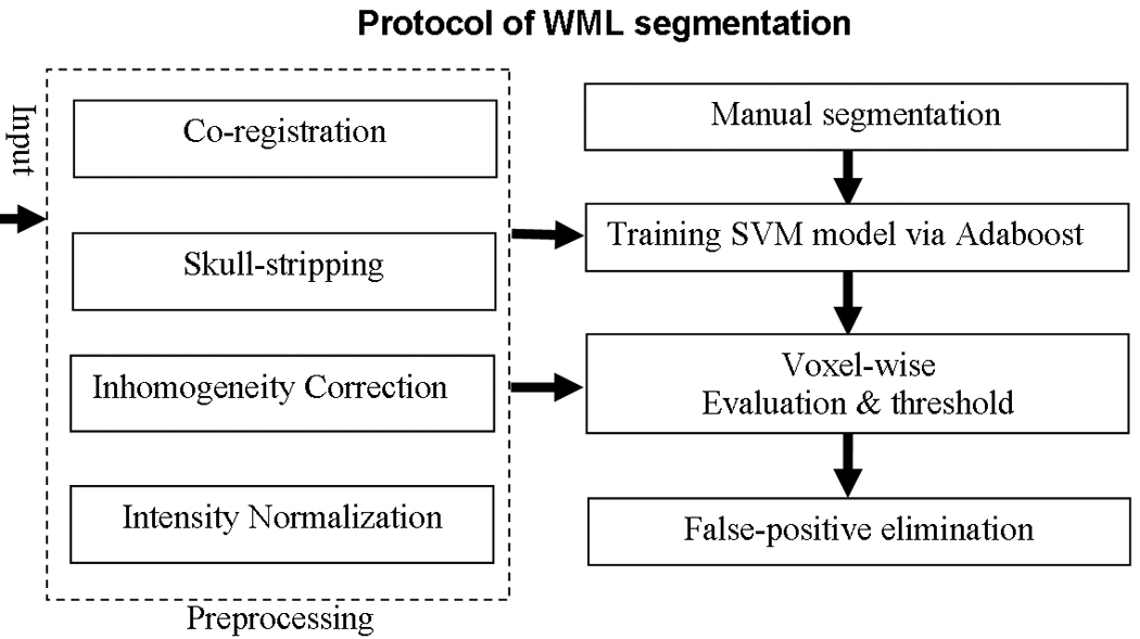
Summary of our computer-assisted WMLs segmentation protocol.

METHODS

Patients and MR Imaging

Images used in this study were offered by the ACCORD-MIND MRI trial, which is a prospective randomized 4-site trial on conventional vs. aggressive treatment of diabetes (http://www.accordtrial.org/). Mean age of these subjects was 62 (mean ± SD: 62.2±5.9, range: 54–77, median: 61). 27 were female and 18 were male. MRI’s were performed during the baseline period upon enrollment into the study. All 45 participants’ exams consisted of transaxial T1-w, T2-w, PD and FLAIR scans. All scans except T1-w were performed with a 3 mm slice thickness, no slice gap, a 240 × 240 mm FOV and a 256 × 256 scan matrix. T1-w scans were performed with a 1.5mm slice thickness, same slice gap, FOV and scan matrix.

Preprocessing

The multiple images acquired from the same individual are co-registered, in order to compensate for possible motion between scans. Mutual-information based affine registration [52], implemented in FSL [53], is employed for co-registration of multi-modality images. The FLAIR image of each subject is used as a reference space, to which all other modality images are transformed. After co-registration, a deformable model based skull-stripping algorithm called BET [54], implemented in FSL [53] is used to generate an initial brain tissue mask from the co-registered T1-w image, and then this brain tissue mask is used to extract the brain region from all other modality images. Finally, for each image volume, inhomogeneities are corrected by N3 [55], and intensity normalization within and across different subjects is minimized by a global histogram matching method. To this end, for two 3D images (or 2D slices) I₁ and I₂ with histograms H_I1 (i) and H_I2 (i), respectively, the transformation, T (T(i) = s × i + t where i is the intensity value before and after transformation T, s and t are scaling and translation parameters of T, respectively), is found so that ${\displaystyle \sum _{i=1}^{i=\text{max}}{\left[H_{I_1}(T(i))-H_{I_2}(i)\right]}^2}$ is minimal, where max is the maximum intensity value.

Training

Manual segmentation

10 training sets with highly variable lesion loads were selected from these 45 ACCORD-MIND participants. WMLs in these subjects were manually segmented by two neuroradiologists (RNB and ERM). The segmentation of the 1^st rater was regarded as the gold standard for training our classifier, while the segmentation of the 2^nd rater was used for evaluating inter-rater agreement and for comparing it against computer-rater agreement.

Attribute vector

In general, the amount of intensity overlap between WMLs and normal tissue varies greatly across different modalities as shown in Fig. 2. In T1-w images, WMLs have intensities similar to GM, and in T2-w and PD images, WMLs look very similar to CSF. Although the FLAIR image has the least intensity overlap between WMLs and normal tissues, it has been suggested in the literature that FLAIR is less sensitive in the posterior fossa [56], may lead to “overestimation” of lesion load, and has a higher inter-vendor variability [57, 58]. Furthermore, FLAIR may present hyperintensity artifacts [59, 60] that might lead to false positives, thereby rendering it difficult to use only the FLAIR images to segment WMLs. Therefore, it is important to integrate information from different modalities, in order to minimize the ambiguity in identifying WMLs from using only a single modality image.

Fig. 2.

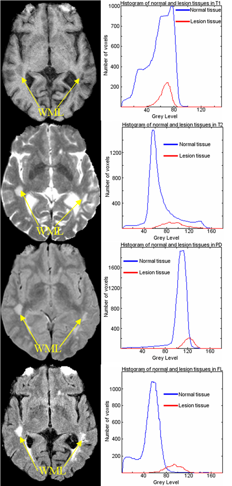
Intensity overlaps between WMLs tissue and normal tissue in T1, T2, PD and FLAIR, respectively (Histograms for normal tissue have been scaled by 0.1 for visualization purpose).

An attribute vector (AV) is computed for each non-background voxel in a 3D reference space for each subject, FLAIR image space serves as the reference space to which all other acquisitions are co-registered. In order to include spatial information from the vicinity of each voxel and make AV robust, each AV includes not only the 4 image intensities of that voxel, but also intensities of neighboring voxels, as shown in Fig. 3. Moreover, to make AV robust to noise, each modality image of the same subject is smoothed by a Gaussian filter with a very small kernel (0.5mm). Mathematically, for a voxel ν in domain Ω, its AV is defined as F(ν)={I^m(μ)}: m ∈ {T₁,T₂,PD, FLAIR}, and μ ∈ B(ν), where B(ν) is a small neighborhood of ν in Ω. In other words, the 4 image intensities of all voxels in the neighborhood of ν are concatenated to an AV. The neighborhood size is selected based on the discrimination ability of AV, in our implementation it is 5mm by 5mm by 5mm. Fig. 4 shows the discrimination ability of this AV with respect to WML. In the figure on the left side, a voxel specified by white cross is selected; in the figure on the right side, the distance in Hilbert space (to be defined later in the paper) between the AV of the marked voxel and the AVs of all other voxels is shown color-coded. It can be seen from the figure that lesion tissue shows high similarity to the selected voxel.

Fig. 3.

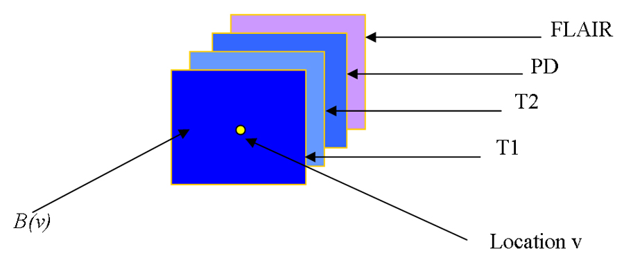
Image intensities from all modalities and all voxels in the spatial neighborhood of a voxel from an AV that serves as an “imaging signature” of each voxel.

Fig. 4.

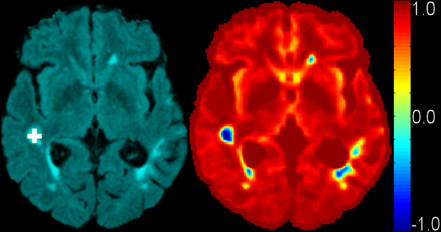
Discrimination ability of AV. Left: FLAIR image with selected lesion voxel marked as white cross. Right: distance distribution in Hilbert space from all other voxels to this selected voxel. AVs of other lesion voxels are similar (having small distance in the attribute space) to the selected voxel, indicating that this imaging signature is characteristic of lesions.

Support Vector Machines (SVM)

SVM are a relatively new machine learning tool and have emerged as a powerful technique for learning from data and in particular, for solving binary classification problems. SVM originate from Vapnik’s statistical learning theory [61] and they formulate the learning problem as a quadratic optimization problem whose error surface is free of local minima and has global optimum. In a binary classification task like the one in our study (normal tissue/lesion tissue), the aim is to find an optimal separating hyperplane (OSH) between the two data sets. Fig. 5 illustrates a two-class problem with a hyperplane separating the two groups. SVM find the OSH by maximizing the margin (minimum distance) between the classes. The main concepts of SVM are to first transform input data into a higher dimensional space (Hilbert Space) by means of a kernel function, and then construct an OSH between the two classes in the transformed space (Hilbert Space). Those data vectors nearest to the constructed line in the transformed space are called the support vectors (Fig. 5) that contain valuable information regarding the OSH. SVM are an approximate implementation of the method of “structural risk minimization” aiming to attain low probability of generalization error. Briefly, the theory of SVM can be referenced in [62].

Fig. 5.

An example of two-class (+ and −) problem showing optimal separating hyperplane (dotted line) that SVM uses to divide two groups’ data, and the associated Support Vectors. Data shown by ‘+’ and ‘−’ represent binary class +1 and −1, respectively.

The kernel function used in our application is Gaussian radial basis function kernel, defined as

$$K(x,y)=\text{exp}\left(\frac{{\Vert x-y\Vert }^2}{2{\alpha }^2}\right)$$

Where x and y are two feature vectors, and α controls the size of the Gaussian kernel.

The fitness of a hyperplane in feature space is usually measured by the distance between the hyperplane and those training points lying closest to it (the support vectors). A consequence of this is that we can completely specify our decision surface in terms of these support vectors. An overview of SVM pattern recognition techniques may be found in [63].

Training SVM via AdaBoost

Once an AV is defined for each location in each training scan, a nonlinear pattern classifier is constructed from the entire training set, i.e. by using all lesion voxels of all training scans as examples of imaging profiles to be recognized in new scans, along with a large number of normal tissue voxels. These example AVs are provided to SVM [64, 65]. Because the number of normal tissue voxels is far higher than the number of lesion voxels, it is essential to select only a representative set of normal tissue voxels comparable to the number of lesion voxels. This selection is not random, but it is rather guided by the classification results themselves, using the AdaBoost algorithm [66]. This approach is based on a sequence of classifiers that rely increasingly on misclassified voxels, since those are presumably the voxels on which the classifier must focus. During this adaptive boosting procedure, each sample receives a weight that determines its probability of being selected in a training set for the next iteration. If a training sample is accurately classified, then its likelihood of being used again in subsequent iterations is reduced; conversely, if a training sample is inaccurately classified, then its likelihood of being used again is increased.

Segmenting a new image

Voxel-wise segmentation of WML by SVM

In the testing stage, T1-w, T2-w and PD images of a new (not in the training set) scan are firstly co-registered to FLAIR space of the subject using mutual-information registration method mentioned before, and then the pseudo-likelihood of each voxel being WML is measured by the generated SVM classifier, as described earlier. The output of SVM is a scalar measure of abnormality (as shown in Fig. 6 left), which is further binarized by an optimal threshold to produce the labels for WMLs (as shown in Fig. 6 right). These labels are called initial WML labels, since false positive labels will be screened out by the methods proposed next.

Fig. 6.

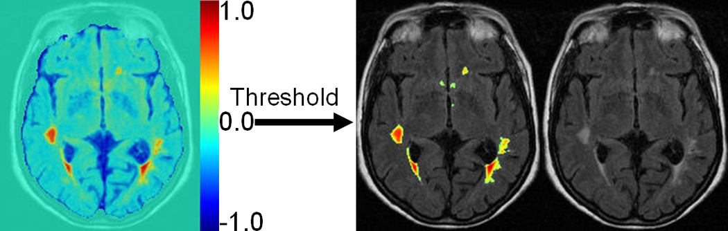
Illustration of voxel-wise segmentation by SVM. Left is the result of voxel-wise evaluation map showing different lesion rating for each voxel, based on generated SVM model (1: lesion; −1: normal). Right is WML segmentation result after thresholding the map on the left superimposed on FLAIR image. Threshold actually corresponds to SVM classification boundary as illustrated in Fig. 7., with 2 classes labeled as −1 and 1 respectively, 0.0 is selected as a threshold.

Elimination of false positive labels

Misregistration between the 4 MR images usually results in a number of false positives around the cortex. This is because of the convoluted nature of the cortex which amplifies the adverse effect of slight registration inaccuracies. By analyzing the spatial distribution of AVs from different samples, we found that AVs of false positive voxels actually form a third class associated with the SVM training samples, which is far away from both classes of lesion and non-lesion training samples. In other words these voxels don't match either lesion or normal tissue, according to the training set. Thus, these false positive voxels can be eliminated to a large extent by computing the distance of their AVs to the training samples in the Hilbert space that the SVM training model was built on, as described before in Support Vector Machine section.

The distance measure in Hilbert space between two vectors ν₁ and ν₂ can be calculated as

$$D_h^2({\nu }_1,{\nu }_2)=K({\nu }_1,{\nu }_1)+K({\nu }_2,{\nu }_2)-2K({\nu }_1,{\nu }_2),$$

where K is the Gaussian kernel function used by the SVM.

Suppose $L=\{{\nu }_i^{\ell },1\le i\le m\}$ is the set of lesion AVs in training samples, m is the total number of AVs in L; $\mathrm{N}=\{{\nu }_i^n,1\le i\le p\}$ is the set of normal tissue AVs in training samples, p is the total number of AVs in N; $F=\{{\nu }_i^f,1\le i\le q\}$ is the set of AVs of false positives, q is the total number of AVs in F. Fig. 7 illustrates the distribution of L, N and F in Hilbert space. Thus, we measure the distance of each AV to a certain set of AVs in the following way. For each ${\nu }_i^{\ell }$, its distance to L in Hilbert space is defined as $d_{{\nu }_i^{\ell }}=\underset{j=1}{\overset{m}{\mathbf{\text{min}}}}{D}_h^2({\nu }_i^{\ell },{\nu }_j^{\ell }),$ where j ≠ i; similarly, for each ${\nu }_i^n$, its distance to N in Hilbert space is defined as $d_{{\nu }_i^n}=\underset{j=1}{\overset{p}{\mathbf{\text{min}}}}{D}_h^2({\nu }_i^n,{\nu }_j^n),$ where j ≠ i; for each ${\nu }_i^f$, its distance to L in Hilbert space is defined as $d_{{\nu }_i^f}^L=\underset{j=1}{\overset{m}{\mathbf{\text{min}}}}{D}_h^2\left({\nu }_i^f,{\nu }_j^{\ell }\right);$ similarly its distance to N in Hilbert space is defined as $d_{{\nu }_i^f}^N=\underset{j=1}{\overset{p}{\mathbf{\text{min}}}}{D}_h^2\left({\nu }_i^f,{\nu }_j^n\right).$ Fig. 8 shows the distributions of these distances, which indicates that we can simply use this minimal distance measure to eliminate the false positive samples, by selecting a suitable threshold.

Fig. 7.

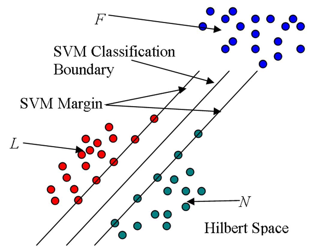
Illustration of L, N and F distribution in Hilbert space. Green and red represent AVs of healthy and lesion tissue, respectively, whereas blue represents AVs of voxels that are misclassified mostly because minor registration errors between the 4 different acquisitions (T1, T2, PD and FLAIR) causes them to have imaging profiles that are drastically different from the training set, and hence prone to misclassification.

Fig. 8.

Demonstration of false positive elimination via AV distance in Hilbert space. (a) Distance distribution of $\{d_{{\nu }_i^{\ell }}\}$ (blue, true positives), $\{d_{{\nu }_i^f}^L\}$ (red, false positives) and the overlap between $\{d_{{\nu }_i^{\ell }}\}$ and $\{d_{{\nu }_i^f}^L\}$ (violet). (b) Distance distribution of $\{d_{{\nu }_i^n}\}$ (blue, true negatives), $\{d_{{\nu }_i^f}^N\}$ (red, false positives) and the overlap between $\{d_{{\nu }_i^n}\}$ and $\{d_{{\nu }_i^f}^N\}$ (violet). WML segmentation results (c) before false positive elimination, and (d) after false positive elimination via thresholding the distance map.

Extra-axial hyperintense regions, like fat in the orbits, can not always be completely removed by the skull-stripping algorithm used in preprocessing stage. Imaging profiles belonging to these regions are more similar to WMLs than that of normal tissue and therefore they are eliminated from the segmentation mask after SVM classification. This is done by morphological operations combined by adaptive thresholding in skull-stripped FLAIR image. Fig. 9 demonstrates one sample result from the algorithm.

Fig. 9.

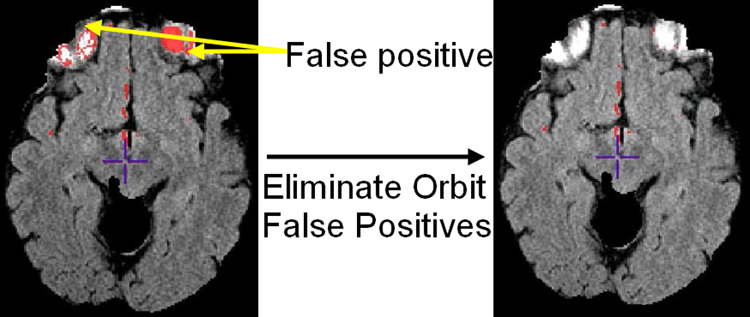
Demonstration of orbital false positive elimination. Left: orbital false positives (red) overlaid on FLAIR before false positive elimination; Right: After orbital false positive elimination.

Results

Two representative results are shown in Fig. 10. “Gold standard” (manual) and computer-assisted segmentation results are superimposed on the FLAIR images, respectively.

Fig. 10.

Comparison of WML segmentation results between gold standard and computer-assisted segmentation for two individual subjects. In subject 1, gold standard and computer-assisted lesion measurements are 11714.9 mm³ and 12397.9 mm³ respectively; in subject 2, gold standard and computer-assisted lesion measures are 15978.5 mm³ and 17884.9 mm³ respectively.

ROC analysis

We have computed the receiver operating characteristic (ROC) curve for our computer-assisted lesion segmentation algorithm. The ROC curve is a graphical plot of the sensitivity vs. (1 - specificity) for a binary classifier system as its discrimination threshold is varied [67]. Fig. 11 shows a zoomed version of ROC curve showing detail in the region of interest. Different symbols on the ROC curve show different thresholds we used. Additionally, “*” shows 2^nd rater’s manual segmentation result, compared to our gold standard.

Fig. 11.

A zoomed part of ROC curve of our segmentation algorithm. The ‘*’ indicates the result of the 2^nd rater compared to gold standard (1^st rater). Other symbols on the curve denote different thresholds, i.e., ‘△’ threshold = −0.15, ‘+’ threshold = 0.0, ‘○’ threshold = 0.05, ‘□’ threshold = 0.2 (see Fig. 6. for definition of threshold).

By investigating the balance between sensitivity and specificity, we determined the optimal threshold to be 0.05. The specificity of an ROC is defined as $\frac{TN}{TN+FP}$, where TN represents the volume of true negatives and FP represents the volume of false positives. In WML segmentation, TN is always a very large number as compared to FP which makes specificity of ROC insensitive to FP change.

Statistical analysis

We trained the classifier on data from 10 participants, and tested it on the remaining 35 cases. We have performed statistical comparisons between the lesion volume obtained by manual and computer-assisted segmentation (with threshold = 0.05) of these 35 subjects. Paired Spearman Correlation (SC) measurements among 1^st rater, 2^nd rater and computer-assisted method shows high correlation among them (p < .001 and ρ = 0.95 between 2^nd rater and 1^st rater; p < .001 and ρ = 0.79 between computer and 1^st rater; p < = .001 and ρ = 0.74 between computer and 2^nd rater). Although high in correlation measurement, mean ± standard deviation (Median) of the lesion volumes obtained from 1^st, 2^nd and computer raters were 1494 mm³ ± 3416 mm³ (559 mm³); 2839 mm³ ± 6192 mm³ (1461 mm³); and 1869 mm³ ± 3416 mm³ (393 mm³) respectively, the mean volume of 2^nd rater is approximate twice of 1^st rater, which suggests that manual segmentation is subject to large inter-rater variability as shown in Fig. 12.

Fig. 12.

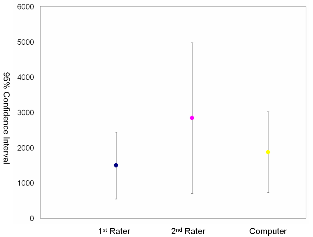
95% CI (Confidence Intervals) for gold standard (1^st rater), 2^nd rater and computer assisted segmentation method (Computer) over 35 subjects respectively. Volume measurements are mm³.

To investigate the variation of the lesion load’s distribution of the 35 evaluated subjects, the coefficient of variation (CV) was calculated. It is a statistical measurement of the dispersion of data around the mean and calculated as: $CV=\frac{\sigma }{\mu }$, where σ is standard deviation and μ is the mean. The CV for the three raters was 189%, 218%, and 182% respectively, which shows that all 3 raters agree on the large variation in lesion load from this set of subjects. Since the distribution of lesion volume is skewed, log transformation (log₁₀) was performed and further statistical analysis was done using the log transformed data. Comparisons between means of the log transformed lesion load (volume in mm³) among raters were performed using paired t-test. On average, the mean of 1^st rater reading was .37 (log₁₀ mm³) lower than 2^nd rater (p < .001), and not significantly higher by .07 (log₁₀ mm³) than computer rater (p <.001). The 2^nd rater’s reading was significantly higher (p < .001) than the computer rater by .38 (log₁₀ cc). The agreement between the computer rater and the 1^st rater is better than that between 2^nd rater and 1^st rater. Computer assisted segmentation is an extension of human rater’s power to more accurately and precisely quantification lesion volume.

Discussion

We have presented an approach to the problem of WML segmentation, based on integrating multiple MR acquisitions and training a nonlinear pattern classification algorithm to recognize imaging profiles that are representative of a brain lesion. By combining 4 types of MR acquisition protocols, namely FLAIR, T₂, PD and T₁, a multi-variant imaging signature is constructed for every image voxel, and is subsequently evaluated by a nonlinear pattern classifier. Results that agree well with human experts were obtained.

The objective, quantitative, and reproducible evaluation of WML has been a challenge in many neuroimaging studies. Although qualitative readings have been employed by many studies, the relatively limited sensitivity and inter-rater agreement is an obstacle, particularly in longitudinal studies or in studies seeking to detect subtle effects. Our experiments confirm that, although human experts are relatively internally consistent in what they define as lesion, they can differ considerably between each other; thereby their readings when combined, increases the measurement mean and standard deviation, and therefore decreases study power.

We did not rigorously evaluate the relative value of each acquisition protocol. Although FLAIR provides the best contrast between periventricular WMLs and ventricles, PD helps avoid potential “overestimation” of lesion load that has been observed with the FLAIR sequence, especially in the posterior fossa. PD may also help in eliminating false positive in regions in which FLAIR has hyperintense artifacts. We experimented with different combinations of 3 modalities and observed that the quality of the segmentation deteriorated when omitting any of the 4 image types. Therefore it appears that all 4 protocols carry some discriminatory power, albeit of different degrees.

One of the challenges we faced during the development of the segmentation method was that the number of lesion training voxels that we had available were dramatically smaller than the number of training voxels for healthy tissue, since lesions constitute a very small percentage of the entire brain. Even smaller was the number of voxels that were misclassified. Therefore, a natural bias toward healthy tissue was inevitable. Although one could randomly select an equal number of voxels for training, the bias toward the more frequent tissues would still persist. We overcame this problem by using adaptive boosting, i.e. via an iterative procedure that progressively emphasized voxels being misclassified. Voxels that were incorrectly classified had more likelihood to influence subsequent iterations. Therefore, in the end the classifier was constructed mainly from “difficult to classify” voxels.

Although in the experiments reported herein we mainly used a binary segmentation output, our approach actually derives a continuous spatial map that provides a pseudo-likelihood of each voxel corresponding to abnormal tissue. Such a continuous map can ultimately be a more appropriate way to characterize certain types of tissues, such as periventicular abnormalities, which might present a continuous scale of pathology.

Although an extensive experimental comparison between this approach and alternative methods in the literature is beyond the scope of this paper, our algorithm has several features that render it novel and likely to be relatively more robust. In particular, we used the currently most robust machine learning method, i.s. SVM, which is known to provide optimal generalization ability. Moreover, we used Adaboost, which is a significant aspect of our approach, since it progressively learns from misclassified examples. Put simply, instead of weighting all voxels similarly, the “difficult” ones are identified by the algorithm, which places relatively more emphasis on them. Automated removal of falase positives via examination of the distance in the Hilbert space is also an important novelty of our approach; this step is most often performed manually in a post-processing step.

The framework of our method is somewhat similar to Abeeck’s approach [44]. Methodologically, both approaches start with a number of pre-processing steps (intra-subject coregistration, skull stripping, inhomogeneity correction, and intensity normalization), and use a supervised classifier (KNN in Anbeek’s approach, SVM here) to separate lesions from normal brain tissue. The key difference is AV definition. In Anbeek’s approach, both intensity and spatial information are used in AV definition. Due to the arbitrary occurrence nature of WML, it’s kind of difficult to form a “complete” training set that covers all occurrences in practice; our approach uses only intensity in AV definition, combined with Adaboost based training samples selection method, thus is easier in forming a “complete” empirical training set. KNN is known to be computational intensive with high dimensional AV, that’s why the AV definition in Anbeek’s approach includes intensity and spatial features only on a single voxel, which may make such AV definition vulnerable to misregistration. SVM does not have such limitation and our AV definition includes not only multi-spectral signals on a certain voxel but also its small neighborhood which makes it more robust to mis-registration.

Several improvements and extensions to our basic methodology are possible. In particular, the current algorithm examines the data voxel-by-voxel, with the exception of using some signal information from a small neighborhood around each voxel. The anatomical context around each voxel could potentially help improve accuracy and reduce false positives. In our previous work [46], we have used a statistical atlas derived from deformable registration of many images of healthy individuals without any pathology, and we detected abnormalities as deviations from the normal spatial variation of healthy tissue. We anticipate that adding such statistically-based anatomical information to the signal-based information examined herein, is likely to improve segmentation accuracy. A second direction of work that might benefit the segmentation is toward co-registration among different modalities. The mutual information based co-registration method we are currently using provides a pair-wise alignment between two modalities. A better way would align images of all modalities simultaneously to reach a consistent solution. Although the smoothing procedure in our WML segmentation protocol performed pretty well in dealing with co-registration error, this step can be improved by a neighborhood voting strategy, i.e. for a certain voxel, measuring the correlation of selected AVs in the neighborhood across different modalities to AVs in the training set and selecting the one with the highest correlation coefficient. This will lead to more robust AVs, and more accurate segmentation result.

In summary, by combining 4 different MR acquisition protocols, and using them to train a nonlinear pattern classification technique, we developed a relatively robust and fully automated segmentation method for white matter abnormalities. We are currently in the process of applying this method to data from over a dozen different centers in multi-site studies, and have obtained stable results, which further bolsters our confidence that this approach can facilitate large-scale neuroimaging studies seeking to quantify vascular disease.

REFERENCES

- 1.Prins ND, et al. Cerebral White Matter Lesions and the Risk of Dementia. Archives of Neurology. 2004;61(10):1531–1534. doi: 10.1001/archneur.61.10.1531. [DOI] [PubMed] [Google Scholar]
- 2.Snowdon DA, et al. Brain infarction and the clinical expression of Alzheimer's disease. The Nun study. JAMA. 1997;277(10):813–817. [PubMed] [Google Scholar]
- 3.Schneider JA, et al. Relation of cerebral infarctions to dementia and cognitive function in older persons. Neurology. 2003;60(7):1082–1088. doi: 10.1212/01.wnl.0000055863.87435.b2. [DOI] [PubMed] [Google Scholar]
- 4.Schneider JA, et al. Cerebral infarctions and the likelihood of dementia from Alzheimer disease pathology. Neurology. 2004;62(7):1148–1155. doi: 10.1212/01.wnl.0000118211.78503.f5. [DOI] [PubMed] [Google Scholar]
- 5.Vermeerx SE, et al. Silent brain infarcts and the risk of dementia and cognitive decline. The new england journal of medicine. 2003;348:1215–1222. doi: 10.1056/NEJMoa022066. [DOI] [PubMed] [Google Scholar]
- 6.Gearing M, et al. The Consortium to Establish a Registry for Alzheimer's Disease (CERAD)Part X. Neuropathology Confirmation of the Clinical Diagnosis of Alzheimer's Disease. Neurology. 1995;45(3):461–466. doi: 10.1212/wnl.45.3.461. [DOI] [PubMed] [Google Scholar]
- 7.Ince P, et al. Neuropathology of a community sample of elderly demented and nondemented people. Brain Pathology. 2000;10:592–593. [Google Scholar]
- 8.Vermeer SE, PN, den Heijer T, Hofman A, Koudstaal PJ, Breteler MM. Silent brain infarcts and the risk of dementia and cognitive decline. N Engl J Med. 2003;348:1215–1222. doi: 10.1056/NEJMoa022066. [DOI] [PubMed] [Google Scholar]
- 9.Zekry D, DC, Moulias R, et al. Degenerative and vascular lesions of the brain have synergistic effects in dementia of the elderly. Acta Neuropathol. 2002;103:418–487. doi: 10.1007/s00401-001-0493-5. [DOI] [PubMed] [Google Scholar]
- 10.Snowdon DA, GL, Mortimer JA, Riley KP, Greiner PA, Markesbery WR. Brain infarction and the clinical expression of Alzheimer disease. JAMA. 1997;277:813–817. [PubMed] [Google Scholar]
- 11.Schneider JA, WR, Bienias JL, Evans DA, Bennett DA. Cerebral infarctions and the likelihood of dementia from Alzheimer disease pathology. Neurology. 2004;13:1148–1155. doi: 10.1212/01.wnl.0000118211.78503.f5. [DOI] [PubMed] [Google Scholar]
- 12.de Groot JC, et al. Cerebral white matter lesions and cognitive function: the Rotterdam Scan Study. Annals of Neurology. 2000;47(2):145–151. doi: 10.1002/1531-8249(200002)47:2<145::aid-ana3>3.3.co;2-g. [DOI] [PubMed] [Google Scholar]
- 13.de Groot JC, et al. Cerebral white matter lesions and depressive symptoms in elderly adults. Archives of General Psychiatry. 2000;57(11):1071–1076. doi: 10.1001/archpsyc.57.11.1071. [DOI] [PubMed] [Google Scholar]
- 14.Longstreth WT, Jr, et al. Clinical correlates of white matter findings on cranial magnetic resonance imaging of 3301 elderly people. The Cardiovascular Health Study. Stroke. 1996;27(8):1274–1282. doi: 10.1161/01.str.27.8.1274. [DOI] [PubMed] [Google Scholar]
- 15.Briley DP, et al. Does leukoaraiosis predict morbidity and mortality? Neurology. 2000;54(1):90–94. doi: 10.1212/wnl.54.1.90. [DOI] [PubMed] [Google Scholar]
- 16.Allen KV, Frier BM, Strachan MWJ. The relationship between type 2 diabetes and cognitive dysfunction: longitudinal studies and their methodological limitations. European Journal of Pharmacology. 2004;490(1–3):169–175. doi: 10.1016/j.ejphar.2004.02.054. [DOI] [PubMed] [Google Scholar]
- 17.Arvanitakis Z, et al. Diabetes mellitus and risk of Alzheimer disease and decline in cognitive function. Archives of Neurology. 2004;61(5):661–666. doi: 10.1001/archneur.61.5.661. [DOI] [PubMed] [Google Scholar]
- 18.Luchsinger JA, et al. Diabetes Mellitus and Risk of Alzheimer's Disease and Dementia with Stroke in a Multiethnic Cohort. American Journal of Epidemiology. 2001;154(7):635–641. doi: 10.1093/aje/154.7.635. [DOI] [PubMed] [Google Scholar]
- 19.Araki Y, et al. MRI of the brain in diabetes mellitus. Neuroradiology. 1994;36(2):101–103. doi: 10.1007/BF00588069. [DOI] [PubMed] [Google Scholar]
- 20.Eguchi K, Kario K, Shimada K. Greater impact of coexistence of hypertension and diabetes on silent cerebral infarcts. Stroke. 2003;34(10):2471–2474. doi: 10.1161/01.STR.0000089684.41902.CD. [DOI] [PubMed] [Google Scholar]
- 21.Heijer T, et al. Type 2 diabetes and atrophy of medial temporal lobe structures on brain MRI. Diabetologia. 2003;46(12):1604–1610. doi: 10.1007/s00125-003-1235-0. [DOI] [PubMed] [Google Scholar]
- 22.Inoue T, et al. Asymptomatic multiple lacunae in diabetics and non-diabetics detected by brain magnetic resonance imaging. Diabetes research and clinical practice. 1996;31(1–3):81–86. doi: 10.1016/0168-8227(96)01196-5. [DOI] [PubMed] [Google Scholar]
- 23.Kariox K, et al. Diabetic brain damage in hypertension: role of renin-angiotensin system. Hypertension. 2005;45(5):887–893. doi: 10.1161/01.HYP.0000163460.07639.3f. [DOI] [PubMed] [Google Scholar]
- 24.Schmidt R, et al. Magnetic Resonance Imaging of the Brain in Diabetes: The Cardiovascular Determinants of Dementia (CASCADE) Study. Diabetes. 2004;53(3):687–692. doi: 10.2337/diabetes.53.3.687. [DOI] [PubMed] [Google Scholar]
- 25.Williamson J, et al. The Action to Control Cardiovascular Risk in Diabetes Memory in Diabetes Study (ACCORD-MIND): Rationale, Design, and Methods. American Journal of Cardiology. 2007 doi: 10.1016/j.amjcard.2007.03.029. [DOI] [PubMed] [Google Scholar]
- 26.Mäntylä R, et al. Variable Agreement Between Visual Rating Scales for White Matter Hyperintensities on MRI Comparison of 13 Rating Scales in a Poststroke Cohort. Stroke. 1997;28(8):1614–1623. doi: 10.1161/01.str.28.8.1614. [DOI] [PubMed] [Google Scholar]
- 27.Bryan RN, et al. A method for using MR to evaluate the effects of cardiovascular disease of the brain: the cardiovascular health study. American journal of Neuroradiology. 1994;15:1625–1633. [PMC free article] [PubMed] [Google Scholar]
- 28.De Groot JC, et al. Periventricular cerebral white matter lesions predict rate of cognitive decline. Annals of Neurology. 2002;52(3):335–341. doi: 10.1002/ana.10294. [DOI] [PubMed] [Google Scholar]
- 29.Benson RR, et al. Older people with impaired mobility have specific loci of periventricular abnormality on MRI. Neurology. 2002;58(1):48–55. doi: 10.1212/wnl.58.1.48. [DOI] [PubMed] [Google Scholar]
- 30.Smith CD, et al. White matter volumes and periventricular white matter hyperintensities in aging and dementia. Neurology. 2000;54(4):838–842. doi: 10.1212/wnl.54.4.838. [DOI] [PubMed] [Google Scholar]
- 31.Kamber M, et al. Model-Based 3-D segmentation of multiple sclerosis lesions in magnetic resonance brain images. IEEE Transactions on Medical Imaging. 1995;14(3):442–453. doi: 10.1109/42.414608. [DOI] [PubMed] [Google Scholar]
- 32.Warfield S, et al. Automatic identification of grey matter structures from MRI to improve the segmentation of white matter lesions; Proc. of the Conf. on Med Rob and Comp Ass. Surg; 1995. [DOI] [PubMed] [Google Scholar]
- 33.Udupa J, Wei L, Samarasekera S, Miki Y, van Buchem MA, Grossman RI. Multiple Sclerosis Lesion Quantification Using Fuzzy-Connectedness Principles. IEEE Transactions on Medical Imaging. 1997;16(5):598–609. doi: 10.1109/42.640750. [DOI] [PubMed] [Google Scholar]
- 34.Welti D, et al. Spatio-temporal segmentation and characterization of active multiple sclerosis lesions in serial MRI data; Proceedings of Information Processing in Medical imaging; 2001. [Google Scholar]
- 35.Zijdenbos AP, et al. Morphometric analysis of white matter lesions in MR images: method and validation. IEEE Transactions on Medical Imaging. 1994;13(4):716–724. doi: 10.1109/42.363096. [DOI] [PubMed] [Google Scholar]
- 36.Alfano B, et al. Automated segmentation and measurement of global white matter lesion volume in patients with multiple sclerosis. Journal of Magnetic Resonance Imaging. 2000;12(6):799–807. doi: 10.1002/1522-2586(200012)12:6<799::aid-jmri2>3.0.co;2-#. [DOI] [PubMed] [Google Scholar]
- 37.Van Leemput K, et al. Automated segmentation of multiple sclerosis lesions by model outlier detection. IEEE Transactions on Medical Imaging. 2001;20(8):677–688. doi: 10.1109/42.938237. [DOI] [PubMed] [Google Scholar]
- 38.Udupa JK, et al. Multiprotocol MR image segmentation in multiple sclerosis: Experience with over 1,000 studies. Academic Radiology. 2001;8(11):1116–1126. doi: 10.1016/S1076-6332(03)80723-7. [DOI] [PubMed] [Google Scholar]
- 39.Leemput KV, et al. Automated Segmentation of Multiple Sclerosis lesions my model outlier detection. KU-Leuven; 2000. [DOI] [PubMed] [Google Scholar]
- 40.Wu Y, et al. Automated segmentation of multiple sclerosis lesion subtypes with multichannel MRI. NeuroImage. 2006;32(3):1205–1215. doi: 10.1016/j.neuroimage.2006.04.211. [DOI] [PubMed] [Google Scholar]
- 41.Zijdenbos AP, Forghani R, Evans AC. Automatic "pipeline" analysis of 3-D MRI data for clinical trials: application to multiple sclerosis. IEEE Transactions on Medical Imaging. 2002;21(10):1280–1291. doi: 10.1109/TMI.2002.806283. [DOI] [PubMed] [Google Scholar]
- 42.Warfield SK, et al. Adaptive, template moderated, spatially varying statistical classification. Medical Image Analysis. 2000;4(1):43–55. doi: 10.1016/s1361-8415(00)00003-7. [DOI] [PubMed] [Google Scholar]
- 43.Wei X, et al. Quantitative Analysis of MRI Signal Abnormalities of Brain White Matter With High Reproducibility and Accuracy. Journal of Magnetic Resonance Imaging. 2002;15(2):203–209. doi: 10.1002/jmri.10053. [DOI] [PubMed] [Google Scholar]
- 44.Anbeek P, et al. Probabilistic segmentation of white matter lesions in MR imaging. NeuroImage. 2004;21(3):1037–1044. doi: 10.1016/j.neuroimage.2003.10.012. [DOI] [PubMed] [Google Scholar]
- 45.Admiraal-Behloul F, et al. Fully automatic segmentation of white matter hyperintensities in MR images of the elderly. NeuroImage. 2005;28(3):607–617. doi: 10.1016/j.neuroimage.2005.06.061. [DOI] [PubMed] [Google Scholar]
- 46.Yu S, et al. ISBI 2004. Arlington, Va.: 2004. Automatic segmentation of white matter lesions in T1-weighted brain MR images. [Google Scholar]
- 47.Anbeek P, et al. Probabilistic segmentation of brain lesion in MR imaging. NeuroImage. 2005;27(4):795–804. doi: 10.1016/j.neuroimage.2005.05.046. [DOI] [PubMed] [Google Scholar]
- 48.Gerig G, et al. MICCAI. Cambridge, MA.: 1999. Exploring the discrimination power of the time domain for segmentation and characterization of lesions in serial MR data. [DOI] [PubMed] [Google Scholar]
- 49.Meier DS, Guttmann CRG. MRI time series modeling of MS lesion development. NeuroImage. 2006;32(2):531–537. doi: 10.1016/j.neuroimage.2006.04.181. [DOI] [PubMed] [Google Scholar]
- 50.Jack CRJ, O'Brien PC. FLAIR Histogram Segmentation for Measurement of Leukoaraiosis Volume. Journal of Magnetic Resonance Imaging. 2001;14:668–676. doi: 10.1002/jmri.10011. [DOI] [PMC free article] [PubMed] [Google Scholar]
- 51.Mohamed FB, et al. Increased differentiation of intracranial white matter lesions by multispectral 3D-tissue segmentation: preliminary results. Magnetic Resonance Imaging. 2001;19(2):207–218. doi: 10.1016/s0730-725x(01)00291-0. [DOI] [PubMed] [Google Scholar]
- 52.Viola P, Wells WM., III . Proceedings of the International Conference in Computer Vision. Los Alamitos, CA.: 1995. Alignment by maximization of mutual information. [Google Scholar]
- 53.Smith SM, et al. Advances in functional and structural MR image analysis and implementation as FSL. NeuroImage. 2004;23(S1):208–219. doi: 10.1016/j.neuroimage.2004.07.051. [DOI] [PubMed] [Google Scholar]
- 54.Smith SM. BET: Brain Extraction Tool. FMRIB technical report TR00SMS26. [Google Scholar]
- 55.Sled J, Zijdenbos A, Evans A. A nonparametric method for automatic correction of intensity nonuniformity in MRI data. IEEE Transactions on Medical Imaging. 1998;17(1):87–97. doi: 10.1109/42.668698. [DOI] [PubMed] [Google Scholar]
- 56.Gawne-Cain ML, et al. MRI lesion volume measurement in multiple sclerosis and its correlation with disability: a comparison of fast fluid attenuated inversion recovery (fFLAIR) and spin echo sequences. J. Neurol. Neurosurg. Psychiatry. 1998 February;64:197–203. doi: 10.1136/jnnp.64.2.197. [DOI] [PMC free article] [PubMed] [Google Scholar]
- 57.Bastianello S, et al. Fast spin-echo and fast fluid-attenuated inversion-recovery versus conventional spin-echo sequences for MR quantification of multiple sclerosis lesions. Am. J. Neuroradiology. 1997;18(4):699–704. [PMC free article] [PubMed] [Google Scholar]
- 58.Rovaris M, et al. Relevance of Hypointense Lesions on Fast Fluid-Attenuated Inversion Recovery MR Images as a Marker of Disease Severity in Cases of Multiple Sclerosis. Am. J. Neuroradiology. 1999;20(5):813–820. [PMC free article] [PubMed] [Google Scholar]
- 59.Bakshi R, et al. Intraventricular CSF Pulsation Artifact on Fast Fluid-Attenuated Inversion-Recovery MR Images: Analysis of 100 Consecutive Normal Studies. Am. J. Neuroradiology. 2000;21(3):503–508. [PMC free article] [PubMed] [Google Scholar]
- 60.Tanaka N, et al. Applicability and Advantages of Flow artifact–insensitive Fluid-attenuated Inversion-recovery MR Sequences for Imaging the Posterior Fossa. Am. J. Neuroradiology. 2000;21(6):1095–1098. [PMC free article] [PubMed] [Google Scholar]
- 61.Vapnik VN. Statistical Learning Theory. Wiley; New York: 1998. p. 736. [Google Scholar]
- 62.Vapnik VN, editor. The Nature of Statistical Learning Theory (Statistics for Engineering and Information Science) 2nd edition. Springer-Verlag; 1999. [Google Scholar]
- 63.Burges CJC. A tutorial on support vector machines for pattern recognition. Data Mining and Knowledge Discovery. 1998;2(2):121–167. [Google Scholar]
- 64.Vapnik VN. Statistical Learning Theory. New York: Wiley; 1998. [Google Scholar]
- 65.Lao Z. Morphological classification of brains via high-dimensional shape transformations and machine learning methods. Neuroimage. 2004;21(1):46–57. doi: 10.1016/j.neuroimage.2003.09.027. [DOI] [PubMed] [Google Scholar]
- 66.Duda RO, Hart PE, Stork DG. Pattern Classification. John Wiley and Sons, Inc; 2001. [Google Scholar]
- 67.Zweig MH, Campbell G. Receiver-operating characteristic (ROC) plots: a fundamental evaluation tool in clinical medicine. Clinical Chemistry. 1993;39(8):561–577. [PubMed] [Google Scholar]