

Abstract
The dynamics of the electric fields in the interior of DNA are measured by using oligonucleotides in which a native base pair is replaced by a dye molecule (coumarin 102) whose emission spectrum is sensitive to the local electric field. Time-resolved measurements of the emission spectrum have been extended to a six decade time range (40 fs to 40 ns) by combining results from time-correlated photon counting, fluorescence up-conversion and transient absorption. Recent results showed that when the reporter is placed in the center of the oligonucleotide, the dynamics are very broadly distributed over this entire time range and do not show specific time constants associated with individual processes [J. Am. Chem. Soc. 2005, 127, 7270]. This paper examines an oligonucleotide with the reporter near its end. The broadly distributed relaxation seen before remains with little attenuation. In addition, a new relaxation with a well defined relaxation time of 5 ps appears. This process is assigned to the rapid component of “fraying” at the end of the helix.
Introduction
An extended DNA double helix is a much more stable and robust structure than an isolated base pair due to cooperative interactions along the helix. However, as part of its biological functioning, these interactions are frequently disrupted: at bulges, junctions, hairpins and so on. How do these disruptions destabilize the nearby helix? The terminus of a helix serves as a prototype for exploring this question. At a helix terminus, the interactions with half of the helix are removed, and some degree of “fraying” is expected. In addition, fraying and other end-effects are inevitably present in oligonucleotides. These short helices are commonly used both as biochemical model systems and as components in building nanostructures. Thus, understanding end effects is an important component of understanding the overall behavior of DNA and oligonucleotides.
The best studied end effect is the intermittent breaking of hydrogen bonds and opening of the terminal base-pair.1,2 However, the terminal base-pair spends only a small fraction of the time in the open state. Another aspect of fraying is that the closed base-pair experiences increased mobility due to the reduced structural constraints at the end of the helix. Evidence for this increased mobility is seen by x-ray crystallography,3 by NMR spectroscopy4–6 and by computer simulation.7–9 However, none of these studies have given specific rates for these extra motions. In addition to increased motion of the terminal base pair itself, the conditions in the interior of the helix may change near the helix terminus due to changes in the nearby solvent and counterions. Water now occupies the space of the missing portion of the helix. In addition, the counterion density is believed to be lower near the end of an oligonucleotide than at its center.10
This paper is concerned with these additional fast dynamics at the end of a DNA helix. We apply the method of time-resolved Stokes shifts (TRSS) to this problem. In a recent letter, we showed that this method can measure dynamics in DNA over a six order-of-magnitude time range from 40 fs to 40 ns.11 In this paper, we extend those experiments to identify the additional dynamics that occur at the end of a DNA helix. TRSS measurements with the probe molecule in the middle of an oligonucleotide are compared to measurements with the probe near the end of the helix over the extended six order-of-magnitude time range.
The TRSS method relies on a chromophore whose spectrum is sensitive to its local environment. Because DNA does not have any suitable native chromophores, we replace a native base pair with a coumarin 102 group12 paired with an abasic-site analog (THF) (Figure 1). The coumarin’s absorption and emission spectra are sensitive to the electric field because coumarin’s excited state has a substantially larger dipole moment than its ground state.13,14 In the presence of a local electric field, the excited state is stabilized more than the ground state, and the electronic transition shifts to lower frequency.
Figure 1.
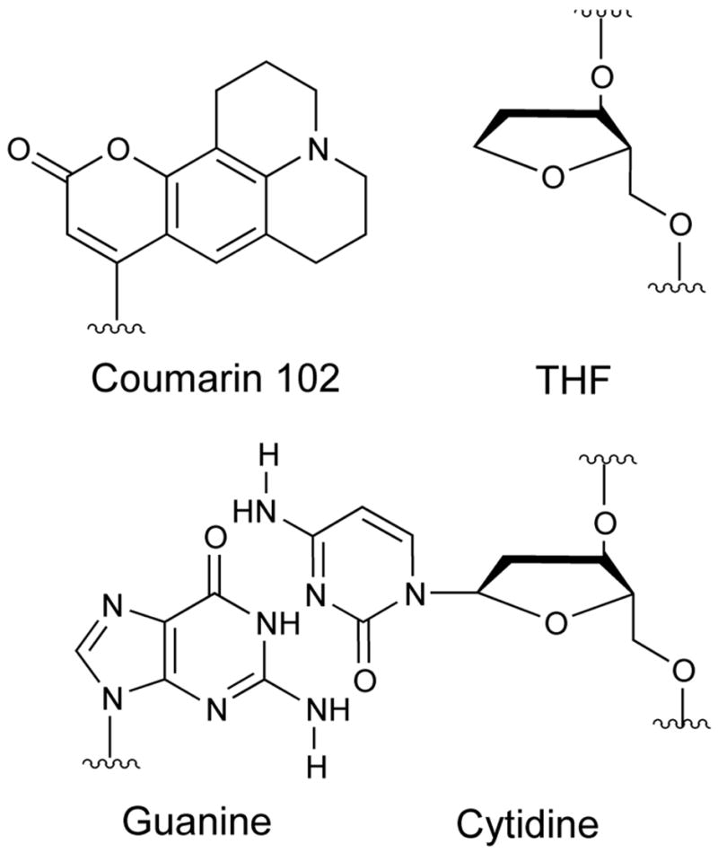
Structures of a native guanine:cytidine base pair (bottom) and of the coumarin:THF base-pair replacement used as a TRSS probe (top).
In a TRSS experiment, the change in dipole moment is used to induce motion as well as to report on the resulting changes in the local electric field. An initial, short light pulse raises coumarin to its excited state. The increased dipole on the coumarin creates a new electric field that extends into the surrounding material and exerts a force on any nearby charge and a torque on any nearby dipole. In DNA, the phosphates, counterions, water and the partial charges on nearby bases all feel this new force and respond by moving to new positions. This movement creates a reaction electric field at the coumarin, which in turn causes a time-dependent shift of the coumarin fluorescence toward lower frequencies.
The TRSS experiment consists of measuring this shift of the fluorescence, i.e., the Stokes shift, as a function of time after excitation. By a linear response argument, the dynamics of the motions induced by the perturbing field of the coumarin are the same as the dynamics of the thermal fluctuations of the unperturbed system.15
A disadvantage of the TRSS experiment in DNA is that the nonnative chromophore may perturb the native DNA properties to some extent. However, the perturbations induced by coumarin appear to be small. Figure 1 suggests that coumarin has a size and shape similar to a native base pair. Molecular modeling confirms this idea: coumarin occupies a position in the DNA helix similar to the position of a native base, and the helix shows little distortion.16 Circular dichroism, melting studies and coumarin spectral shifts in DNA are also consistent with this picture.16 Coumarin-containing oligonucleotides undergo strong and specific binding and cleavage by the APE1 endonuclease.17 It is reasonable to assume that the types of motion seen in coumarin-containing oligonucleotides, their basic time scales and relative amplitudes are representative of the motions in native DNA, even if there is some change in the absolute numbers measured.
Our earlier TRSS studies in DNA focused on the longer times accessible by time-correlated single-photon counting (40 ps to 40 ns), where DNA shows unexpectedly slow relaxation.16–19 Pal, et al. reported on faster motions using fluorescence up-conversion.20
We recently showed that a complete characterization of the TRSS response in DNA requires a combination of measurement techniques to cover six decades in time (40 fs to 40 ns).11 The response over this entire time range can be fit to a simple power-law expression. Recently, similar behavior has been found in a computer simulation of an oligonucleotide that does not contain a nonnative probe.21 The origin of the power-law form is not clear at present. However, it is clear that the data do not show any special time scales that can be associated with specific motions.
In this paper, we compare the TRSS responses over the entire 40 fs – 40 ns time range from two sequences: one with the coumarin probe (coum) in the center of a 17-mer, 5′-GCATGCGC(coum)CGCGTACG-3′ and its complement 5′-CGTACGCG(THF)GCGCAT GC-3′ (centered sequence), and one with the probe in the penultimate position, 5′-C(coum)CGCGTACGGCATGCG-3′ and its complement 5′-CGCATGCCGTACGCG (THF)G-3′ (helix-end sequence). The sequence context of the coumarin is the same in both sequences, except that the helix terminates one base pair after the coumarin in the helix-end sequence. By comparing the two results, we will isolate any additional motions at the terminus of the helix.
Making TRSS measurements over a broad time range requires merging results from different experimental techniques in a self consistent fashion. This procedure introduces special problems that ultimately affect the fits to the data in a significant way. These problems become crucial as we look for small changes in the dynamics as the position of the probe is changed. Therefore, the paper begins with a detailed description of the essential elements in the data analysis.
The results from a probe in the middle of the helix, which have been presented in a previous letter,11 are then reviewed to provide a baseline for comparison to the results with the probe near the helix terminus.
Finally, new measurements with the probe near the helix end are presented. When the probe is placed at the penultimate position in the helix, the power-law dynamics seen in the center of the helix are retained, with only a modest reduction in intensity. In addition, a new process that is well described by a 5 ps single exponential is introduced. We assign this process to fraying motions.
Experimental Methods
Oligonucleotide Preparation
The 17-mers 5′-GCATGCGC(coum)CGCGTACG-3′ (centered sequence) and 5′-C(coum)CGCGTACGGCATGCG-3′ (helix-end sequence) (coum = coumarin-102 C-deoxyriboside) were synthesized as described previously.12,16 The complementary strands, containing an abasic-site analog opposite the coumarin, were purchased commercially. Double stranded DNA was prepared by dissolving the single strands in 100 mM sodium phosphate buffer (pH 7.2) and annealing at 90 °C. No extra salt was added to any of the samples. To reduce scattering from DNA absorbed to the walls, all sample cells were treated with a 5% solution of dimethyldichlorosilane in chloroform prior to use.
Steady-State Spectroscopy
Steady-state emission spectra were excited at 390 nm at the magic angle with a 4 nm bandwidth. Excitation spectra were detected at 500 nm with a 4 nm bandwidth. The raw data were corrected for instrumental effects using quinine sulfate as a standard.22 The standard was run within a few days of the sample measurement and in the same sample cell. The spectra were then converted from intensity versus wavelength to susceptibility versus frequency before further analysis.19
For emission spectra in a glass, glycerol was added to the sample to make a 1:3 solution of buffer:glycerol. The addition of glycerol shifted the spectrum by less than 2 nm. The samples were frozen using a dry ice/acetone bath at a temperature of −78 °C (195 K).
All these spectra, as well as the time-resolved spectra discussed later, are converted from intensity and absorbance versus wavelength to susceptibility χ versus frequency ν.19 For absorption and excitation spectra χ ∝ ε/ν. For emission spectra, the intensity in radiometric units I(λ) (W/nm) are first converted to units of photons/cm−1, Iν (ν) ∝ I(λ)/ν3, and then converted to susceptibility, χ ∝ Iν (ν)/ν3 This scale corrects for frequency dependent factors in the spectral intensities and allows absorption, spontaneous-fluorescence and stimulated-emission spectra to be compared directly and quantitatively.
Time-Resolved Spectroscopy
Time-resolved emission spectra were measured by three different techniques: time-correlated single-photon counting23 (TCSPC) from 40 ps to 40 ns, fluorescence upconversion24 from 1 ps to 150 ps and stimulated-emission spectra derived from transient-absorption (TA) spectra from 40 fs to 125 ps.
A standard experimental setup was used for the TCSPC. Briefly, light pulses from a mode-locked Ti:sapphire laser (~100 fs) were selected at 6 MHz and frequency-doubled to 390 nm. The sample fluorescence was excited by 4 mW of this light. Fluorescence was collected at right angles, polarized at magic angle, dispersed in a 0.22 meter single monochromator and detected by a multichannel-plate detector. Single-photon events were timed with standard electronics23 to yield fluorescence decay data at 12 wavelengths. The typical instrument response function was 45 ps FWHM. The sample had a concentration of 45 μM in coumarin (helices). The static sample cell was held in a temperature regulated sample holder at 15 °C. In a typical decay, 3×10⁷ photons were collected. Sample degradation was not noticeable over the period of data collection.
The broadband TA setup has also been described in detail elsewhere.25,26 The samples were excited at 160 Hz by 1–2 μJ pulses at 403 nm focused to a 200 μm spot. The change in absorption was measured using a white-light probe pulse focused to 100 μm and at magic-angle polarization. Signals from pure solvent were measured and subtracted from the data to remove the solvent electronic and Raman contributions. The peak in time of the solvent signal was taken as the zero point of time for each wavelength. The temporal width of the Raman signals was 60 fs, indicating the time resolution of the technique. Multiple scans were checked for consistency and then averaged. Data collected with various temporal step sizes and ranges were combined and averaged in bins that are evenly spaced in logarithmic time.11 The TA samples were 1 mM in coumarin/helices and 0.5 M in buffer and were held in a specially fabricated 400 μm thick cell with 200 μm thick silanized silica windows. The sample was circulated slowly during the experiment. The sample was kept at 17 °C by regulating the room temperature.
The upconversion data were obtained from a home-built instrument. A home-built Ti: sapphire oscillator produced 65 fs pulses with an average power of 250 mW. This beam was frequency doubled to produce a beam at 395 nm with an average power of 15 mW, which was used to excite the sample. The remaining light at 800 nm was used as the gate for the upconversion. After excitation, the fluorescence was collected by an off-axis parabolic mirror and refocused by a second parabolic mirror onto a 1 mm thick β-BBO crystal. The second parabolic mirror also focused the gate pulse on the BBO crystal. The sum-frequency beam was collected by a 50 mm silica lens, the stray light was removed by a 1 mm Schott Glass UG-11 filter and the signal was dispersed by a single monochromator with a 300 grooves/mm grating blazed at 300 nm. The signal was detected by standard photon-counting electronics.
The up-conversion sample was stirred and kept under flowing nitrogen in a standard 1 mm cuvette. The sample was kept at 25 °C by regulating the room temperature. With a sample concentration of 1.5 mM in coumarin, a volume of 100 μL and an excitation power of 15 mW, loss of absorption due to sample degradation was significant and limited the data collection time to 4 hrs. Scans moving forward and backward in delay were averaged to correct for the small signal loss during a single scan.
Merging Data from Different Techniques
TRSS experiments in DNA present special problems because the dynamics are spread over a wide range of time scales. To the best of our knowledge, TRSS has not been previously applied to such a broad time range. Several different techniques must be used to cover the entire time range. The results from these techniques must be combined in a self-consistent manner to avoid introducing artifacts in the matching procedure. At the longest measured time, the system is still not fully equilibrated, so the common assumption that the steady-state spectrum is the equilibrium spectrum cannot be made. The need for to avoid artifacts and to achieve good accuracy is heightened in the current experiments, where differences between samples with small structural changes are being measured. For these reasons, we describe the data analysis in some detail in this section.
Steady-state spectroscopy
The analysis starts with steady-state spectra, which are shown in Figure 2. The emission spectra in the glass are shifted to lower frequency than the absorption spectra as a result of vibronic structure, fast vibrational relaxation in the excited state and emission of phonons into the glass. None of these very rapid dynamics are of concern to this paper; we wish to focus on diffusive dynamics, those dynamics that cannot be described as quasi-harmonic vibrations. Diffusive dynamic are described as outer-sphere reorganization in the context of electron-transfer theory or as non-inertial dynamics in the context of liquid dynamics.
Figure 2.
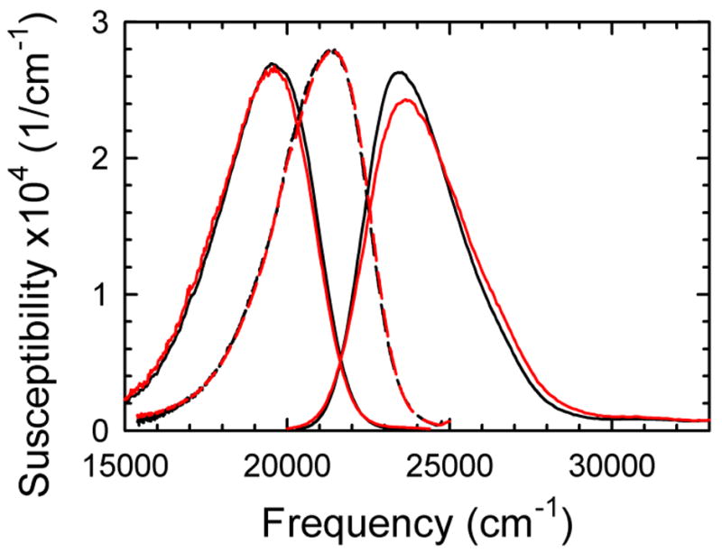
Steady-state excitation (right), emission at room temperature (left) and emission in a glass (middle) for the centered (black) and helix-end (red) sequences. The differences between the steady-state spectra of the two sequences are small. Normalized to unit area.
We use the position of the glass spectra as the zero point for measuring Stokes shifts. Assuming that there are no spectral shifts due to addition of the cryogen or due to the low temperature of the glass, this “absolute Stokes shift” scale measures the total amplitude of diffusive dynamics and removes the effects of rapid vibrational dynamics. We expect our measurements to extrapolate to zero absolute Stokes shift at zero time.
Time-correlated single-photon counting
Time-correlated single-photon counting (TCSPC) has a modest time resolution (45 ps), but has the sensitivity to follow the fluorescence spectrum to long times, typically four to five excited-state lifetimes (> 40 ns) (Figure 3). Data is collected as decays at individual wavelengths. Excited-state population relaxation causes a common decay at all wavelengths; the difference between decays at different wavelengths is to due to shifting of the emission spectrum with time.
Figure 3.
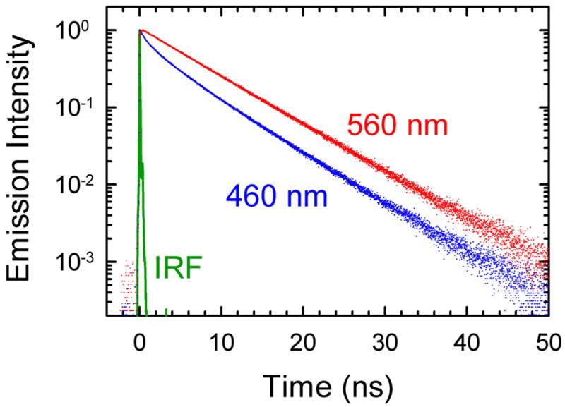
Examples of time-correlated single-photon counting data. Fluorescence decays on the high frequency (blue: 460 nm = 21 740 cm−1) and low frequency (red: 560 nm = 17 860 cm−1) sides of the emission spectrum and the instrument response function (IRF, green) are shown. The decays differ due to the TRSS effect. This effect is clearly present at these long times and can be followed accurately out to several times the fluorescence lifetime. These data are from the centered sequence.
Time-correlated single-photon counting data are converted to a time-dependent Stokes shift by standard methods.13 The data are fit to a multiexponential decay convolved with the instrument response function. The time-dependent emission spectrum is reconstructed by scaling the intensity of each fit so that the time-integration of the time-dependent spectrum matches the steady-state emission spectrum (Figure 2). The procedures for interpolating between wavelength points and for extrapolating the wings of the spectrum have been described previously.19
We do not rely on results shorter than the instrument response function. Replicas of the entire experiment provide estimates of the total range of errors and the maximum time before those errors diverge.27 The Stokes shifts derived from TCSPC data have an estimated error range of ± 30 cm−1 (two standard deviations) out to 40 ns.
Transient absorption
Transient absorption (TA) can have very high time resolution, although its moderate sensitivity and the need for optical delay lines limit its utility at long times. Here, TA data is used from 40 fs to 125 ps.
As measured, TA data are in the form of time-resolved spectra (Figure 4A). Unlike TCSPC data, there is no need for elaborate spectral reconstruction. However, the TA spectrum Δ χTA(ω, t) contains three overlapping contributions: stimulated emission χEm(ω, t), ground-state bleaching χBl(ω, t) [Ed: el (not one) in subscript] and excited-state absorption χEx(ω, t). These three individual components are shown at 65 ps in Figure 4B. (The decomposition procedure is described below.) The stimulated emission is dominant in the region 17 000 to 22 000 cm−1, whereas the ground-state bleach dominates from 22 000 to 25 000 cm−1. Excited-state absorption, which has the opposite sign from the other two components, is the largest component in the region above 25 000 cm−1, but contributes throughout the spectral region shown. The evolution with time of the raw TA spectra is clear in Figure 4B and is primarily due to the TRSS of the stimulated emission.
Figure 4.
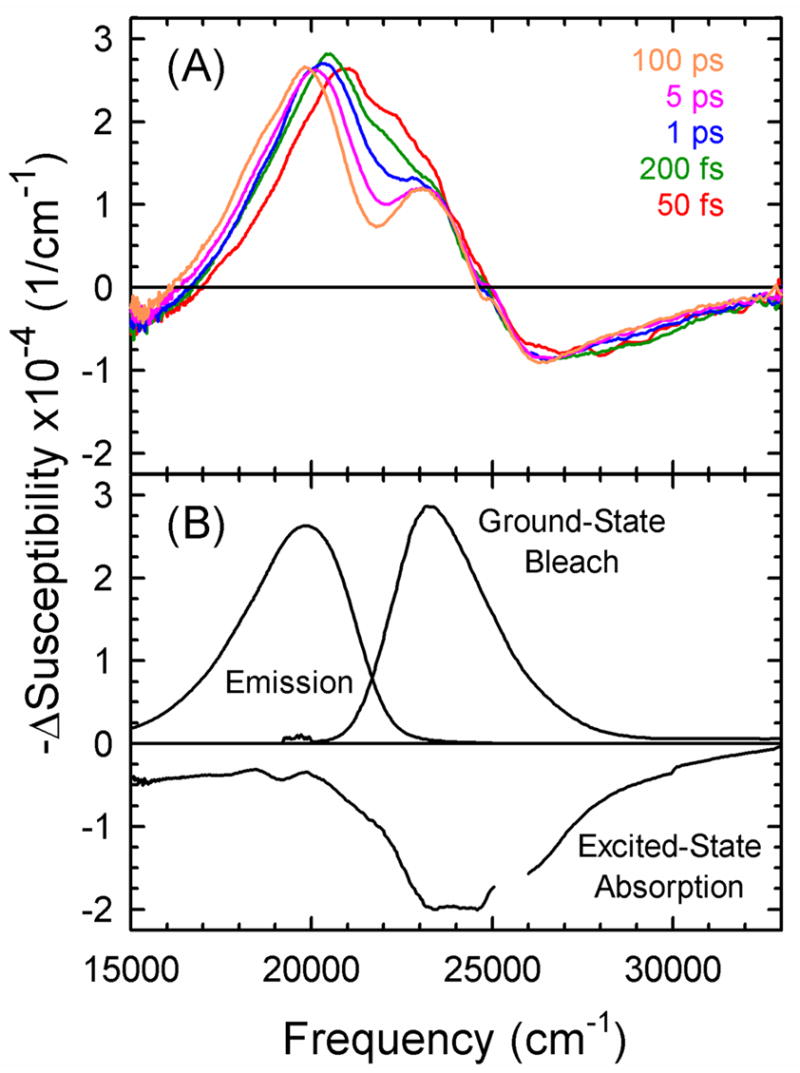
(A) Typical transient-absorption spectra at various times show large changes at early times. (B) The individual components making up the transient-absorption spectrum at 65 ps: stimulated emission, ground-state bleach and excited-state absorption. The Stokes shift of the stimulated emission dominates the changes in the transient-absorption spectra with time. These data are from the centered sequence. Each spectrum has been normalized to unit area.
The stimulated-emission spectra are extracted from the TA spectra using the equation
| (1) |
The bar indicates spectra that have been normalized to unit area. The fact that the areas of the absorption and stimulated-emission spectra (i.e., their transition strengths) are equal has been used. The ratio of the transition strengths of the excited-state absorption and the ground-state absorption is κ. Equation 1 approximates the ground-state bleach with the steady-state absorption χBl(ω, t) = χAb(ω). This approximation neglects vibrational cooling, and it neglects hole-burning effects, which are avoided in the experiment by excitation into the vibronically crowded portion of the ground-state absorption spectrum.
In many systems, the value of κ can be determined at long times, where the emission spectrum is no longer evolving and can be taken to be equal to the steady-state emission spectrum. Because of the long equilibration times in DNA, we cannot use this procedure. Instead, we determine κ by using the emission spectrum from TCSPC at a time where the TCSPC and TA data overlap.
We made the determination at 65 ps, in the middle of the overlap in time ranges. An excited-state spectrum is found from eq 1 by assuming a value of κ, using the TCSPC spectrum for the emission component and the steady-state absorption spectrum for the ground-state bleach,. Figure 5 shows three examples assuming different values of κ. If κ is too large (e.g., κ = 1.6), a distinct peak remains at the position of the overlap of the absorption and emission spectra, near 20 000 cm−1. If κ is too small (e.g., κ = 1.3), the spectrum develops a negative region, which is physically impossible, or more subtly, it develops a valley at the position of absorption and emission overlap. An optimal value of κ = 1.45 is found, but there is some subjectivity within a range around this value.
Figure 5.
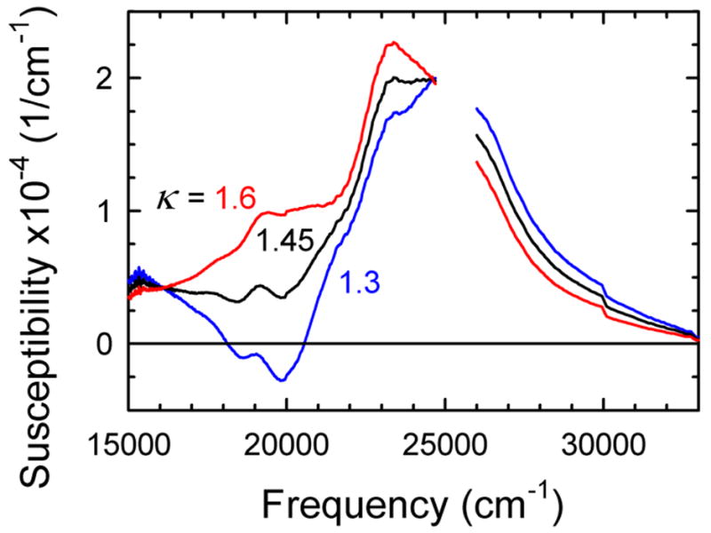
Excited-state absorption spectrum assuming various values of κ, the strength of the excited-state absorption relative to the strength of the ground-state absorption. The value κ = 1.45 gives the most reasonable spectral shape and is used in the rest of the analysis. The spectra are normalized to unit area. These data are from the centered sequence at 65 ps. The region near the pump frequency (25 000 cm−1) is perturbed by scattered light and has been left blank.
Often the time dependence of the excited-state absorption can be neglected. In that approximation, the excited-state absorption derived at 65 ps and the experimental absorption spectrum are subtracted from the TA spectrum at every time to yield the time-dependent stimulated-emission spectrum. The validity of this approximation is tested in the next subsection.
Fluorescence up-conversion and time-dependent excited-state absorption
Although the above procedures make the emission spectrum from TCSPC and TA agree at 65 ps by construction, they do not eliminate the concerns in matching the data from different techniques. Both techniques involve substantial data analysis: TCSPC relies on deconvolution and smoothing procedures; TA invokes several reasonable, but untested assumptions. If one of the techniques approaches the cross-over time with the incorrect slope, the resulting break in the slope could be misinterpreted as a dynamical process near that time. If the determination of the excited-state absorption, which relies on short time TCSPC data, is distorted, systematic errors might propagate throughout the TA time range.
To test for these types of problems, we performed fluorescence up-conversion measurements on the centered sequence (Figure 6). These measurements extend from 1 ps to 150 ps, overlapping well with both the TA and TCSPC data. The decays at different wavelengths were scaled in amplitude to match the emission spectrum from TCSPC at 65 ps. The instrument response function is less than 0.5 ps, so no deconvolution was required. There are no ground-state or excited-state absorption components to subtract from the data. The upconversion data can be interpreted with a minimum of data manipulation.
Figure 6.
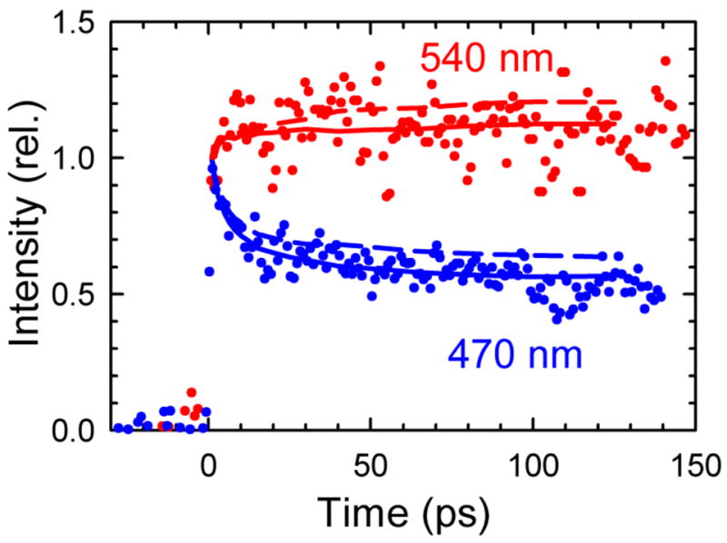
Examples of fluorescence up-conversion data (points) on the high frequency (blue: 470 nm = 21 280 cm−1) and low frequency (red: 540 nm = 18 520 cm−1) sides of the emission spectrum are quite different, indicating a pronounced Stokes shift at intermediate times. The stimulated-emission decays extracted from transient-absorption data (lines) do not agree well if shifting of the excited-state absorption spectrum is ignored (α = 0, dashed), but do agree if this shift is accounted for (α = 1, solid). These data are from the centered sequence.
Unfortunately, up-conversion is an inefficient process, which limits the signal-to-noise ratio. In principle, longer data collection times could improve the noise, but photodegradation and the small amount of sample available limited the collection times.
The initial agreement of the up-conversion data with TA results was marginal. This is illustrated in Figure 6, which shows the up-conversion results at two wavelengths compared to the emission decays at those wavelengths derived from the TA spectra when analyzed as described above (α = 0). The TA decays fall within the scatter of the up-conversion data, but do not run through the middle of the data.
The most severe approximation made in analyzing the TA data is that the excited-state absorption does not shift in time. In principle, the excited-state absorption spectrum is shifted by the same reaction field that produces the Stokes shift of the emission spectrum. Thus, we assume
| (2) |
The excited-state absorption spectrum at time t is the spectrum determined at 65 ps, shifted by an amount δω. This shift is taken to be proportional to the Stokes shift of the emission spectrum S(t) relative to its value at 65 ps, with the proportionality constant α. If the final state of the excited-state absorption Sn has the same dipole moment as S1, then the excited-state absorption does not shift, and α = 0. On the other hand, if Sn has the same dipole moment as S0, then the excited-state absorption shifts at the same rate as the emission spectrum, although in the opposite direction (α = 1).
An iterative procedure was used to solve the combination of eqs 1 and 2. An initial Stokes shift was derived using eq 1 and neglecting the shift of the excited-state absorption (α = 0). This initial Stokes shift was used in eq 2 along with an assumed value of α to produce an improved estimate of the time-dependent excited-state absorption. Iterating between eqs 1 and 2 produced full convergence within 5–6 cycles. Changing the value of α changed the level of agreement between the stimulated-emission and up-conversion results. The value of α also changed the position and width of the earliest stimulated-emission spectrum (40 fs), which can be compared to the steady-state emission spectrum in the glass.
The S1 state of coumarin has an unusually large dipole moment, so a priori one expects the Sn dipole moment to be closer to the S0 dipole moment, i.e., α > 0. Using α = 0.5–1.0 gives improved results: the agreement between the TA and up-conversion is better (Figure 6), the Stokes shifts from the three methods match more smoothly, and the short-time emission spectrum is closer to the spectrum in the glass (see Supporting Information). However, it is not possible to determine the value of α more precisely. Value between α = 1 to α = 0.5 all give reasonable results. However, as we shall see below, the final TRSS results changes somewhat within this range (Figure 9 below).
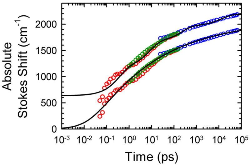
Figure 9.
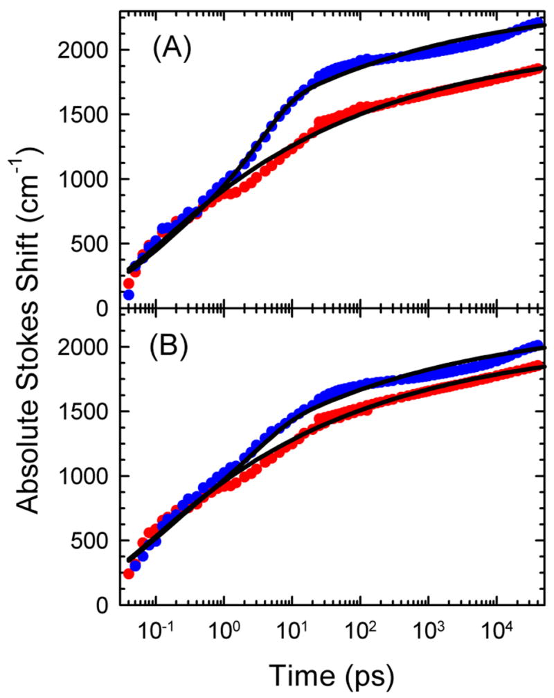
Comparison of TRSS results from the centered sequence (red) and the helix-end sequence (blue) and fits (black) to eq 5. Results are shown for two possible values for the relative magnitude of the excited-state absorption shift: (A) α = 1 and (B) α = 0.5. In (B), the helix-end data have been shifted vertically by +200 cm−1. There is no shift between the data sets in (A).
Despite this small ambiguity, the overall matching of the three different techniques is very good. Examples of the time-resolved emission spectra from the three techniques are compared in Figure 7. The earliest measured spectrum (40 fs) is close to the spectrum in the glass (0 fs), as expected. The final TRSS results, consisting of the first moments of these spectra minus the first moment of the spectrum in the glass, are shown in Figure 8. The results from each of the three techniques agree at 65 ps by construction, but the smoothness of agreement over the rest of the overlap region is a sign of the consistency of the different measurements.
Figure 7.
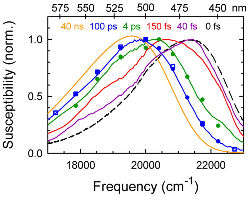
Time-resolved spectra from various techniques show Stokes shifting over the entire time range from 40 fs to 40 ns. The steady-state spectrum in the glass (dashed curve) is used as an estimate of the 0 fs limit of the spectral shift. The spectra are from transient absorption (solid) at 40 fs, 150 fs, 4 ps and 100 ps, from fluorescence up-conversion (circles) at 4 ps and 100 ps and from time-correlated single-photon counting at 100 ps (squares) and 40 ns (solid). The data shown are from the centered sequence with α = 0.5.
Figure 8.
Combined TRSS results from time-correlated single-photon counting (blue points), fluorescence up-conversion (green points) and transient absorption (red points). The lower set of points is fit (black curve) to a power law (eq 3). The upper set of points has been shifted vertically by 300 cm−1 and fit to a sum of four exponentials. The data shown are from the centered sequence with α = 0.5.
Results
Centered Sequence
The final TRSS results for the centered sequence are shown in Figure 8. These results have been presented previously, but because they form the baseline for discussing the helix-end sequence, the main features are reviewed here.
The first important result is that shifting occurs throughout the six-decade range of the measurements. This fact is already evident in the raw data from each technique (Figures 3, 4 and 6) and in the time-resolved spectra (Figure 7).
The final quantified results in Figure 8 also show that the data are smooth on the logarithmic time plot. There are no steps or breaks to indicate special time scales. An exponential relaxation gives a distinct step at the characteristic relaxation time when the data are plotted on a logarithmic time axis. A stretched exponential also gives a step, although a broader one. A sum of a sufficient number of exponentials can mimic the smooth behavior of the data. A minimum of four exponentials is needed as shown in Figure 8. However, remnants of steps at the four time constants remain in the fit, but are not seen in the data. Ultimately a multiexponential fit to the data is not satisfactory. Because the data do not contain identifiable features to fix the time constants at specific times, the fitting parameters are not unique, and there is no reason to believe that they correctly represent the underlying physical processes.
A simpler fitting function for the TRSS S(t) is the power-law
| (3) |
which is shown fit to the data in Figure 8 with n = 0.15±0.03, S∞ = 2060 cm−1 and t0 = 25 fs. This fit has three parameters, compared to the eight parameters of the four exponential fit.
The parameter t0 indicates a cut-off time for the power law. Without it, the fit would diverge when extrapolated to t = 0, a physically unreasonable result. The fit has been constructed to reach zero on the absolute Stokes shift scale at t = 0. This feature is not required by the data (see Supporting Information), but it is consistent with the data. (Note that the four-exponential fit does not go to zero at t = 0).
The parameter S∞ gives the total range of the Stokes shift (recalling our exclusion of vibrational or inertial processes). The data only reach 90% of this value at 40 ns; the value from the fit is a modest extrapolation.
With the proviso that both the long and short time limiting values of the fit are extrapolations, the solvation correlation function can be constructed from eq 3
| (4) |
The limiting form of eq 4, which applies to most of the data, is a very simple power law that contains no important time constants.
The power-law fit is purely empirical; no theoretical explanation exists at present. Power-law dynamics have been seen in other systems: geminate recombination,28 protein relaxation,28 dynamics near critical points or weak first-order transitions.29 However, the relationship between those systems and DNA is not clear. The magnitude of the power law exponent in DNA, n = 0.15, is also very low in comparison to other the exponents seen in other systems.
As an empirical description, the power-law fit is a good representation of the data. It represents in a quantitative fashion that the dynamics are spread evenly over a broad range of times. We will use this function as the baseline for analyzing the additional dynamics introduced at the end of the helix.
Helix-end sequence
Figure 9 compares the TRSS results from the helix-end sequence to those from the centered sequence using two different values of α in the data analysis. Regardless of the value of α, the difference between the two sequences is clear. The power-law dynamics of the centered sequence are largely preserved at the helix end, but there is an additional relaxation at the helix end. This extra relaxation occurs in a well defined period between 1 and 20 ps.
The helix-end data have been fit by combining the power-law relaxation of the centered sequence with a single-exponential decay
| (5) |
The power-law parameters n, t0 and S∞ have been determined by fitting the centered sequence (with A = 1 and B = 0) and are kept the same for the helix-end sequence; only the relative amplitudes of the power-law and exponential relaxations, A and B, and the exponential time constant τ have been adjusted for the helix-end sequence.
Both fits in Figure 9 use τ = 5 ps. This time is assigned to the fraying motions that are unique to the end of the helix. Unlike the power-law dynamics, this motion has single, well-defined relaxation time. This result suggests that the fraying motions are localized motions that are only weakly coupled to the dynamics of the rest of the system.
The relative amplitudes of the background power-law dynamics and the fraying motions are sensitive to the value of α used in the data analysis. At one end of the acceptable range, α = 1.0 (Figure 9A), the fraying amplitude is 15% of the power-law component. With this value of α, the data before 1 ps match for both sequences, as is expected.
At the other end of the acceptable range, α = 0.5, the amplitude of the fraying component is reduced by a factor of two, to 7% of the power-law component (Figure 9B). In this fit, the early time data from the two sequences do not match without additional adjustment. The helix-end data have been shifted +200 cm−1 to make this match. We cannot exclude the possibility of a systematic error of this size. Although there is some uncertainty in the magnitude of the fraying component, it is not possible to eliminate it completely without creating inconsistencies elsewhere in the data analysis.
In a previous study using only TCSPC data at times greater than 40 ps, we noted small differences between results with the centered and helix-end sequence.19 Those differences are minor compared to the change revealed in this study over a broader time range. The current fits have neglected those small changes, and their physical significance needs further investigation.
Discussion and Conclusions
TRSS experiments show a distinct relaxation process associated with the end of the helix, a relaxation that constitutes the rapid component of the fraying of the oligonucleotide at its terminus. Unlike the broadly distributed power-law dynamics that are seen everywhere in the oligonucleotide, the fraying has a well defined time of 5 ps. Previous NMR measurements have detected an increased amplitude of motion at the ends of oligonucleotides in the picosecond time range, but could not isolate a time constant for this motion.4–6
X-ray,3 NMR4–6 and computer7–9 experiments agree that fraying is largely confined to the last two base-pairs, with most of the motion on the terminal base pair. Two general types of motion can be envisioned, each of which could be detected in a TRSS experiment. Without the steric constraints of neighboring bases on one side, rolling, buckling and propeller twisting of the terminal base pair should be enhanced. These motions would allow greater solvent access to the coumarin probe in the penultimate position. This solvent motion would affect the electric field at the probe, allowing the motion to be detected in a TRSS experiment. Alternatively, winding/unwinding motion of the helix would cause large movements of the terminal phosphates. Because the phosphates are charged, this motion would also cause changes in the electric field at the probe and thereby would be detected in a TRSS experiment. In the computer simulation of Young, et al., the phosphates show the largest increase in motion at the helix terminus.8 Thus, these simulations suggest that winding/unwinding motions dominate. More detailed analysis of simulations for the type of motion enhanced at the helix terminus and particularly for the rates of these motions would assist in the interpretation of the TRSS results.
In addition to the new motions induced at the end of the helix, it is also interesting to consider what happens to the “normal” dynamics seen in the middle of the helix when the probe is translated to the helix terminus. The power-law relaxation that occurs in the middle of the helix persists at the end of the helix with no change in the power-law exponent and only a minor reduction in amplitude to 75–90% of its value in the center (see Supporting Information). Because the entire helix beyond the probe’s nearest neighbor has been removed and replace with solvent, the power-law relaxation must arise from interactions on a fairly short range, approximately the distance to its neighboring bases. This inference is supported by computer simulations that suggest an effective interaction range of ~15 Å.21
The unusually long TRSS times in DNA raises the possibility that the power-law relaxation is due to a long range interaction along the one dimensional helix. As examples, ion diffusion along the helix or bending and writhing motions of the helix sensed by long range interactions with phosphates could be imagined as sources of the long relaxation times. However, these types of long range interactions would be changed significantly when the probe is near the end of the helix. Because the power-law relaxation is not strongly perturbed at the helix terminus, such long range mechanisms cannot be the cause of the slow relaxation.
The overall message from these results is that the changes in dynamics at the end of the helix are quite modest, so long at the terminal base pair remains closed. The power-law dynamics seen in the center of the helix persist with only a small reduction in amplitude. The new motions induced at the terminus has a small amplitude compared to these pre-existing dynamics. Increased mobility of the final base-pair, motion of the backbone ends and increased solvent accessibility have only a small effect, even on the penultimate site. We can infer that other types of disruption of the helical structure; bulges, hairpins, junctions, and so on; will only change the dynamics in a very localized portion of the helix.
Moreover the increased range of conformations allowed at the helix end is sampled very quickly, within about 5 ps. This time is too fast to be the time for opening and closing of the final base pair. It is close to the time that would be needed to move water around the structure in response to a base opening. For base opening to be this fast, it would need to be essentially barrierless. The base-opening time is known to be faster than 1 ms from proton-exchange measurements.1 From the lack of any longer time features in the TRSS experiments, we can also say that this time is longer than 40 ns.
In our samples, a certain fraction of the oligomers will be in the open state. As just discussed, our results do not show that actual kinetics of opening and closing. However, they do show a weighted average of the dynamics within the closed state and within any open structures present. In a native oligomer, about 3% of a terminal CG pair are open at 0 °C and 12% at 25 °C.2 Given that the probe increases the melting temperature of an oligonucleotide by 13 °C,16 our samples are probably at the high end of this range.
Given that the relative amplitude of the new exponential feature seen at the helix end is in this same range, it is possible to argue that our results for the helix-end sequence consist of an unperturbed power law for the closed state and a 5 ps exponential and no power-law component for the open state. This interpretation calls for an extreme difference between the dynamics of the two states. More likely, the response due to the open state has a sufficiently small amplitude and is sufficiently similar to the closed state dynamics that the open state response cannot be discerned within the data.
This study has also revealed the technical requirements for the use of TRSS to measure how changes in the structure of DNA change its dynamics. The baseline dynamics of unmodified DNA extend over six decades in time. Because the changes due to modifications are likely to have an amplitude less than the baseline dynamics, measurements with high accuracy and self consistency over this entire range are needed.
The techniques used here were adequate to meet these requirements, but also showed limitations. In particular, transient absorption measurements are susceptible to systematic errors due to the need to subtract large contributions from ground-state bleaching and excited-state absorption. Fluorescence up-conversion can provide high time resolution emission spectra without interfering contributions. However, the low efficiency of conversion from absorbed photons to detected emission becomes a problem with samples that are available in limited supply. Photodecomposition occurs with an efficiency that effectively competes with the detection of upconverted photons and thereby limits the signal-to-noise level of upconversion measurements.
A new up-conversion method developed by some of the current authors, broadband up-conversion, promises to alleviate these problems.30 By using a near-IR gate pulse, a carefully selected up-conversion crystal and a tilted gate pulse, the bandwidth and angular acceptance of the upconversion process are dramatically increased. The ratio of detected to absorbed photons is improved by 6000 fold compared to the measurements reported here. In addition, spectral properties are measured more self-consistently, because the entire spectrum is measured at the same time. With these technical advances, systematic studies of the relationship between DNA structure and dynamics over the entire femtosecond to nanosecond range will be possible through TRSS measurements.
Supplementary Material
Effect of α on early TRSS spectra. Effect of changing t0 in fits to eq 3. Comparison of excited-state absorption spectra of both sequences. Table of fitting parameters. This material is available free of charge at http://pubs.acs.org
Acknowledgments
This work was supported by the National Institutes of Health (GM-61292).
References
- 1.Leroy JL, Kochoyan M, Huynhdinh T, Guéron M. J Mol Biol. 1988;200:223. doi: 10.1016/0022-2836(88)90236-7. [DOI] [PubMed] [Google Scholar]
- 2.Nonin S, Leroy JL, Guéron M. Biochemistry. 1995;34:10652. doi: 10.1021/bi00033a041. [DOI] [PubMed] [Google Scholar]
- 3.Holbrook SR, Kim SH. J Mol Biol. 1984;173:361. doi: 10.1016/0022-2836(84)90126-8. [DOI] [PubMed] [Google Scholar]
- 4.Fujimoto BS, Willie ST, Reid BR, Schurr JM. J Mag Res B. 1995;106:64. doi: 10.1006/jmrb.1995.1009. [DOI] [PubMed] [Google Scholar]
- 5.Borer PN, Laplante SR, Kumar A, Zanatta N, Martin A, Hakkinen A, Levy GC. Biochemistry. 1994;33:2441. doi: 10.1021/bi00175a012. [DOI] [PubMed] [Google Scholar]
- 6.Kojima C, Ono A, Kainosho M, James TL. J Mag Res. 1998;135:310. doi: 10.1006/jmre.1998.1584. [DOI] [PubMed] [Google Scholar]
- 7.Norberg J, Nilsson L. J Chem Phys. 1996;104:6052. [Google Scholar]
- 8.Young MA, Ravishanker G, Beveridge DL. Biophys J. 1997;73:2313. doi: 10.1016/S0006-3495(97)78263-8. [DOI] [PMC free article] [PubMed] [Google Scholar]
- 9.Norberg J, Nilsson L. Biophys J. 2000;79:1537. doi: 10.1016/S0006-3495(00)76405-8. [DOI] [PMC free article] [PubMed] [Google Scholar]
- 10.Anderson CF, Record MT. Annu Rev Phys Chem. 1995;46:657. doi: 10.1146/annurev.pc.46.100195.003301. [DOI] [PubMed] [Google Scholar]
- 11.Andreatta D, Pérez Lustres JL, Kovalenko SA, Ernsting NP, Murphy CJ, Coleman RS, Berg MA. J Am Chem Soc. 2005;127:7270. doi: 10.1021/ja044177v. [DOI] [PubMed] [Google Scholar]
- 12.Coleman RS, Madaras ML. J Org Chem. 1998;63:5700. [Google Scholar]
- 13.Maroncelli M, Fleming GR. J Chem Phys. 1987;86:6221. [Google Scholar]
- 14.Moog RS, Davis WW, Ostrowski SG, Wilson GL. Chem Phys Lett. 1999;299:265. [Google Scholar]
- 15.Chandler D. Introduction to Modern Statistical Mechanics. Oxford University Press; New York: 1987. [Google Scholar]
- 16.Brauns EB, Madaras ML, Coleman RS, Murphy CJ, Berg MA. J Am Chem Soc. 1999;121:11644. [Google Scholar]
- 17.Sen S, Paraggio NA, Gearheart LA, Connor EE, Issa A, Coleman RS, Wilson DM, III, Wyatt MD, Berg MA. Biophys J. 2005;89:4129. doi: 10.1529/biophysj.105.062695. [DOI] [PMC free article] [PubMed] [Google Scholar]
- 18.Brauns EB, Madaras ML, Coleman RS, Murphy CJ, Berg MA. Phys Rev Lett. 2002;88:158101. doi: 10.1103/PhysRevLett.88.158101. [DOI] [PubMed] [Google Scholar]
- 19.Somoza MI, Andreatta D, Coleman RS, Murphy CJ, Berg MA. Nucleic Acids Res. 2004;32:2495. doi: 10.1093/nar/gkh577. [DOI] [PMC free article] [PubMed] [Google Scholar]
- 20.Pal SK, Zhao L, Xia T, Zewail AH. Proc Natl Acad Sci USA. 2003;100:13746. doi: 10.1073/pnas.2336222100. [DOI] [PMC free article] [PubMed] [Google Scholar]
- 21.Sen S, Andreatta D, Ponomarev SY, Beveridge DL, Berg MA. doi: 10.1021/ja805405a. in preparation. [DOI] [PMC free article] [PubMed] [Google Scholar]
- 22.Velapoldi RA, Mielenz KD. Standard Reference Materials: A Fluorescence Standard Reference Material: Quinine Sulfate Dihydrate. U.S. Government Printing Office; Washington DC: 1980. [Google Scholar]; Nat Bur Stand (US), Spec Publ. :260–64. [Google Scholar]
- 23.Birch DS, Imhof RE. In: Time-Domain Fluorescence Spectroscopy Using Time-Correlated Single-Photon Counting. Lakowicz JR, editor. Plenum Press; New York: 1991. p. 1. [Google Scholar]
- 24.Shah J. IEEE J Quantum Electron. 1988;24:276. [Google Scholar]
- 25.Ernsting NP, Kovalenko SA, Senyushkina T, Saam J, Farztdinov V. J Phys Chem A. 2001;105:3443. [Google Scholar]
- 26.Kovalenko SA, Dobryakov AL, Ruthmann J, Ernsting NP. Phys Rev A. 1999;59:2369. [Google Scholar]
- 27.Sen S, Gearheart L, Rivers E, Lui H, Coleman RS, Murphy CJ, Berg MA. submitted for publication. [Google Scholar]
- 28.Leiderman P, Ben-Ziv M, Genosar L, Huppert D, Solntsev KM, Tolbert LM. J Phys Chem B. 2004;108:8043. [Google Scholar]
- 29.Sengupta A, Fayer MD. J Chem Phys. 1995;102:4193. [Google Scholar]
- 30.Zhao L, Lustres JLP, Farztdinov V, Ernsting NP. Phys Chem Chem Phys. 2005;7:1716. doi: 10.1039/b500108k. [DOI] [PubMed] [Google Scholar]
Associated Data
This section collects any data citations, data availability statements, or supplementary materials included in this article.
Supplementary Materials
Effect of α on early TRSS spectra. Effect of changing t0 in fits to eq 3. Comparison of excited-state absorption spectra of both sequences. Table of fitting parameters. This material is available free of charge at http://pubs.acs.org