

Abstract
Determining how a particular neuron, or population of neurons, encodes information in their spike trains is not a trivial problem, because multiple coding schemes exist and are not necessarily mutually exclusive. Coding schemes generally fall into one of two broad categories, which we refer to as rate and temporal coding. In rate coding schemes, information is encoded in the variations of the average firing rate of the spike train. In contrast, in temporal coding schemes, information is encoded in the specific timing of the individual spikes that comprise the train. Here, we describe a method for testing the presence of temporal encoding of information. Suppose that a set of original spike trains is given. First, surrogate spike trains are generated by randomizing each of the original spike trains subject to the following constraints: the local average firing rate is approximately preserved, while the overall average firing rate and the distribution of primary interspike intervals are perfectly preserved. These constraints ensure that any rate coding of information present in the original spike trains is preserved in the members of the surrogate population. The null-hypothesis is rejected when additional information is found to be present in the original spike trains, implying that temporal coding is present. The method is validated using artificial data, and then demonstrated using real neuronal data.
Keywords: Spike trains, rate coding, temporal coding, simultaneous coding, cricket, cerebellum, multielectrode, synchrony
Introduction
It has long been accepted that neurons encode information in their spike trains (Perkel and Bullock, 1968). Many studies have shown that neurons encode information in their average firing rates. Indeed, rate coding is the implicitly assumed method of neuronal coding in most studies, even those in which the average firing rate is obtained within a short time window by using an ensemble of neurons (Shadlen and Newsome, 1998; Mar et al., 1999; van Rossum et al., 2002). Yet, the presence of rate coding does not preclude the possibility of encoding information in other ways. In fact, neuronal spiking is reproducible with a precision on the order of a millisecond (Bryant and Segundo, 1976; Mainen and Sejnowski, 1995; van Steveninck et al., 1997; Strong et al., 1998; MacLeod et al., 1998; Reinagel and Reid, 2000), suggesting that the timing of each spike could convey significant information. Schemes where the precise timing of spikes carries information are referred to as temporal coding schemes. It has been argued that temporal coding allows information to be processed at higher speeds with less energy than does rate coding (Abeles, 1991; Thorpe et al., 1996).
In spite of much investigation, however, determining the encoding mechanisms used in particular cases has remained a difficult problem. A major contributor to this problem is that these two types of coding (rate versus temporal) are not necessarily mutually exclusive, so that both may be used by a neuron or network. Moreover, some models and experimental data suggest that neurons may switch between a rate or temporal coding scheme based on certain parameters, such as noise levels, network heterogeneity, and input correlations (Abeles, 1991; Araki and Aihara, 2001; Lu et al., 2001; van Rossum et al., 2002; Tiesinga et al., 2002; Masuda and Aihara, 2002, 2003, 2004). In this paper, we provide a method for detecting the presence of temporal encoding regardless of whether rate coding is also present. Our method is based on using surrogate data, which are widely used for hypothesis testing in nonlinear time series analysis (Scheinkman and LeBaron, 1989; Theiler et al., 1992; Schreiber and Schmitz, 1996; Small et al., 2001), which is similar to the Monte Carlo method in statistics (Press et al., 1988). Here, the surrogate data set represents a population of spike trains with average local firing rates close to those of the original spike trains. The original spike trains and those of their surrogate data can be compared using various statistics that detect the presence of non-rate coding mechanisms.
Methods
Surrogate data are widely used for hypothesis testing in nonlinear time series analysis (Scheinkman and LeBaron, 1989; Theiler et al., 1992; Schreiber and Schmitz, 1996; Small et al., 2001), and are defined as alternate data sets generated from the original true data set. These surrogate data vary in some manner from the original data, while at the same time preserve specific properties of the original data.
In general, to use surrogate data for hypothesis testing, a null-hypothesis is set. Based on this null-hypothesis, specific characteristics of the spike trains are preserved, while others are randomized to generate new data sets (surrogates). These surrogates form a population that allows statistical testing of the properties of the original data set. That is, by checking whether a test statistic obtained from the original time series is within the confidence interval obtained from the surrogate data or not, we either accept or reject the null-hypothesis, respectively. Hypotheses often used include serial dependence (Scheinkman and LeBaron, 1989), nonlinearity (Theiler et al., 1992; Schreiber and Schmitz, 1996), and long term correlations (Small et al., 2001).
Rate coding surrogate
To address the specific problem of neuronal coding, we take as the null-hypothesis that the set of spike trains uses only rate coding, because rejection of the null-hypothesis would imply the presence of other types of coding. Therefore, we need to generate a set of surrogate data that preserve the short-term average firing rate approximately and the overall firing rate exactly. The distribution of interspike intervals will also be preserved perfectly in the method described below. Because the short-term average firing rate throughout the spike train is essentially preserved during surrogate data generation, any information encoded in the short-term average firing rate is also preserved in the surrogates. In contrast, any information present in the specific timing of the spikes in the train is lost. Thus, any statistically significant difference in information content between the sets of surrogates and the set of the original spike trains is the result of non-rate coding mechanism being used.
The distribution of interspike intervals can be easily preserved by generating surrogates by randomly exchanging interspike intervals. This process, however, would not preserve the short-term average firing rate. To preserve the latter, we used a numerical optimization method as next described.
We start by defining the short-term average firing rate mathematically. Let τ be a time window during which spikes are averaged, and s and s̃ be different spike trains for the same time period [0, T). By s[t1,t2), we mean spike train s for time period [t1, t2) ⊂ [0, T ). Let #(s[t1,t2)) denote the number of spikes in s[t1,t2). The number M is the minimum integer satisfying Mτ ≥ T. Then we define the short-term average firing rates of the spike train s by a series {#(s[(j–1)τ, jτ)))/τ|j = 1, 2, , M}.
To describe the algorithm for generating randomized data, we also need to define the distance between two short-term average firing rates. Thus, we introduce the following distance dτ (s, s̃) between s and s̃:
| (1) |
Let p be a permutation for a sequence of interspike intervals. By sp, we denote the spike train whose interspike intervals have been reordered according to p. As only interspike intervals are reordered, the timing for the first and last spikes does not change. If dτ (s, sp) = 0, then sp preserves the short-term average firing rates as well as the distribution of interspike intervals. Therefore, when dτ (s, sp) is small enough, then sp is a good approximation for s with respect to the rate coding on the time scale of τ.
This problem of generating suitable surrogate data can be formulated as a minimization problem over permutation, the same as was done for the general class of surrogate data (Schreiber, 1998). By following Schreiber (1998), we use simulated annealing for minimizing dτ (s, sp) over p. The algorithm can be stated as follows:
Step (1) Generate s0 from the original spike train s by randomly reordering the interspike intervals;
Step (2) Generate si+1 from the newest spike train si by a permutation of interspike intervals. For this sake, choose one of the following procedures with equal probability:
a: exchange the orders of two interspike intervals and keep the other orders the same (See Fig. 1. The details on how to choose two interspike intervals are discussed later.) or
b: exchange an interspike interval with a set of two successive interspike intervals and keep the other orders the same (See Fig. 2. How to choose these interspike intervals is described later.);
Fig. 1.
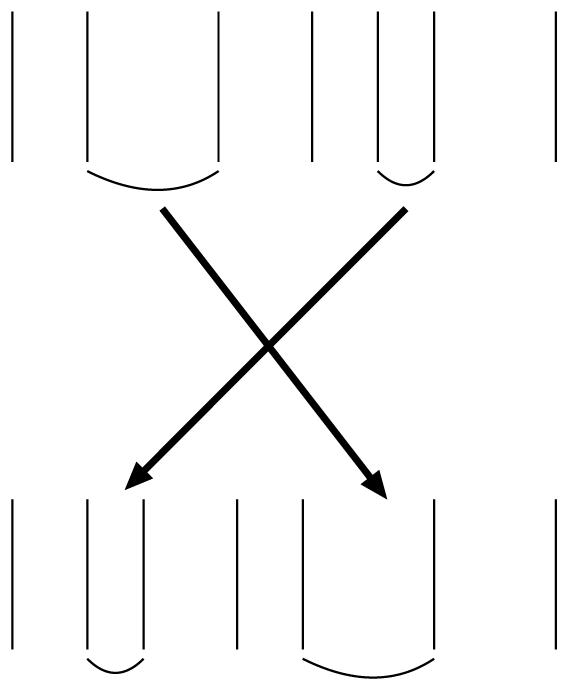
Exchanging the orders of two interspike intervals. The figure shows one of the procedures that was used for generating rate coding surrogates. The upper spike train is changed into a new spike train by the exchange of two randomly chosen interspike intervals.
Fig. 2.
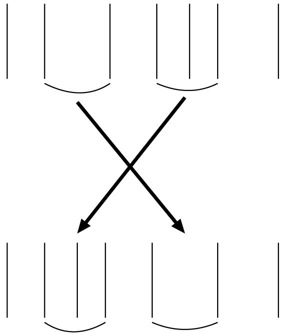
Exchanging an interspike interval with two successive interspike intervals. Another procedure that was used for generating rate coding surrogates is illustrated. In this case one randomly chosen interspike interval is switched with two successive intervals whose combined duration is close to its duration.
Step (3) If dτ (s, si) ≥ dτ (s, si+1), then keep si+1 with a probability of 1. If the new spike train si+1 is worse, namely, dτ (s, si) < dτ (s, si+1), reject si+1 and replace it with si with a certain probability. Specifically, set si+1 ← si with a probability of 1 – exp(– βi(dτ (s, si+1) – dτ (s, si)), where β is a parameter that determines the speed of cooling in the simulated annealing process (Gershenfeld, 1999) and thus how quickly the probability of keeping si+1 when dτ (s, si) < dτ (s, si+1) converges to zero as the number of iterations increases.
Step (4) If the current spike train does not change for 1 000 000 iterations, end the iteration process and take si as a surrogate spike train. Otherwise increment i and go back to Step (2):
In Step (2), we choose either a or b because by choosing a or b, one can avoid local minima of dτ (s, si) more efficiently than by just using one of them.
At Step (2)a, we may choose two interspike intervals randomly. But if this approach is used, it takes long time to decrease dτ (s, si). To speed up the algorithm, in the following applications, we conduct Step (2)a as follows:
Step (2)a: choosing two interspike intervals and exchanging their order.
- 1: Select an interspike interval: Choose the m-th bin with probability
where #(si[a,b))) is the number of spikes in spike train si within time [a, b), and h(x) = 1 if x > 0 and h(x) = 0 otherwise. Then choose randomly an interspike interval that ends within the m-th bin.(2) - 2: Select another interspike interval: Choose the m-th bin with probability
Then choose randomly an interspike interval that ends within the m-th bin.(3) 3: Exchange the interspike intervals selected above.
Note that in Steps (2)a1 and (2)a2 the probability of choosing a bin with no spikes was set to zero. Thus bins without spikes are not selected.
The parameter ρ is set to 0.1 throughout the applications. Step (2)a1 tends to select an interspike interval in a bin where s contains more spikes than si: It follows from Eq. (2), if a bin [(m − 1)τ, mτ) contains more spikes in s than in si, a chance for choosing the bin becomes higher and thus the chance for choosing an interspike interval related to that bin gets higher. The denominator of Eq. (2) normalizes the probabilities. In contrast, Step (2)a2 tends to select an interspike interval in a bin where s contains fewer spikes than si because Eq. (3) raises the selection probability for bins where s contains fewer spikes than si. If we exchange a pair of interspike intervals one of which is in a bin where s has more spikes than si and the other is in a bin where s has fewer spikes than si, there is a higher chance that we can make the numbers of spikes close to those of the original spike train in the two bins. Thus, Eqs. (2) and (3) help in choosing more appropriate pairs of interspike intervals for exchanging.
As for Step (2)b, we first choose two consecutive interspike intervals randomly. Then we choose another interspike interval whose length is close to the sum of the two consecutive interspike intervals. Mathematically, this process can be written as follows: Let I(s, j) be the j-th interspike interval of spike train s. Let j be the first interspike interval of the two chosen consecutive interspike intervals. Then we choose the k-th interspike interval (k ≠ j, j + 1) by using the following probability:
| (4) |
Then we exchange the j-th and (j + 1)-th interspike intervals with the k-th interspike interval. In this paper, we set ø = 0.1.
At Step (3), simulated annealing was employed because there are lots of local minima in dτ (s, si) as a function of si. During the procedure of simulated annealing, even when dτ (s, si) does not decrease, we sometimes still use the new order, si+1, so that we can overcome local minima. In these cases the probability of keeping si+1, the new spike order, was exp(–βi(dτ (s, si+1) – dτ (s, si+1))). This expression has several desirable features. For example, as the number of iterations, i, increases, the probability of keeping a new order whose dτ (s, si+1) is worse than the one of the current si decreases, which is desirable because in earlier stages of the procedure it is more likely that si is trapped by a local minimum, and thus we want to dispose of the previous spike train si more often, but as the iterations increase being trapped in an unacceptable local minimum becomes less likely. The probability of replacing si with si+1 when dτ (s, si+1) > dτ (s, si) also decreases as the magnitude of the difference, dτ (s, si+1) – dτ(s, si), increases, which also makes sense because the larger this difference, the more likely is si+1 to be a worse solution than is si. In this paper, we set β = 0.1.
In Step (3), the temperature of the annealing process is proportional to 1/i and thus it converges to 0 from the above along the number of iterations.
We call the spike train generated by the above algorithm a rate coding surrogate on the time scale of τ, or simply a rate coding surrogate. This process is repeated to generate a population of surrogates, to which the original spike train or set of trains may be compared.
Test statistics
To test the surrogate method for its ability to detect the presence of temporal coding in spike trains, two statistics were used that should be sensitive to the precise timing of spikes within an individual neuron's spike train or across multiple spike trains.
Prediction error
The first statistic is a prediction error. Prediction error quantifies how well an upcoming spike time can be predicted from past ones. If the precise spike times are random, then the times for a set of spikes provide no information about the specific times of other spikes. However, if the spike times do contain meaningful contents, some estimate of the upcoming spike time may be possible from the preceding spikes.
For a population of cells, the prediction error for interspike intervals was calculated by first combining the individual spike trains from all of the cells into a single spike train. Next, the nearest neighbor for each set of consecutive interspike intervals was found. Then, the prediction is given by the interspike interval following the most recent interspike interval that forms the vector of the nearest neighbor. The specific algorithm is as follows:
(1) Obtain the interspike intervals from the spike train of each neuron and concatenate the interspike intervals obtained from all neurons into a single series (Fig. 3). Let Tk be the k-th interspike interval of the concatenated series, where k runs between 1 and N and N is the total number of interspike intervals.
(2) Form a vector (Tk, Tk−1, Tk−2, Tk−3, Tk−4) for each k between 5 and (N − 1).
(3) For each k between 5 and (N − 1), find the index n(k) from a set of indexes {5, 6, ..., k −1, k +1, ..., N − 1} that corresponds to the closest vector (Tn(k), Tn(k)−1, Tn(k)−2, Tn(k)−3, Tn(k)−4) to (Tk, Tk−1, Tk−2, Tk−3, Tk−4) in the Euclidean distance. Let Tn(k)+1 be a prediction for Tk+1 (Fig. 4).
(4) The prediction error is then the mean of |Tk+1 − Tn(k)+1| over k.
Fig. 3.
The first and second steps in the algorithm for obtaining the first test statistic, the prediction error, are shown. If there are some repeated spatio-temporal patterns in spike trains, then the prediction error is reduced. For example, in this figure, the second spike of each neuron has a delay of 2.65 from the first one, and the third one has a delay of 3.56 from the second one. Thus, in the concatenated series of interspike intervals, 2.65 and 3.56 are repeated, which makes the prediction error smaller. Because the spike train in this example is so short it is not possible to take five consecutive interspike intervals, but this is not generally an issue since in most instances spike trains will be made up of a much larger number of intervals.
Fig. 4.
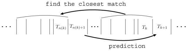
The third step for obtaining the first test statistic, the prediction error. With each current vector of 5 consecutive interspike intervals, all vectors of 5 consecutive interspike intervals are compared to find the most similar. Then the interspike interval following the most similar vector provides a prediction for the interspike interval following the current vector.
If there is temporal structure in the original spike trains that is beyond variations in local average firing rate, the prediction error for the original spike trains will tend to be smaller than that for rate coding surrogates, because the randomization process used to generate the surrogates destroys the additional temporal structure. We decided to use the 5-dimensional vectors for finding the closest match because the number of dimensions for the vectors should be large enough to specify the context but still allow the vectors to be reasonably close neighbors from a given dataset.
Compression ratio of spike trains
The second test statistic is given by the compressed file sizes of the spike train expressed as interspike intervals. The compressed file sizes quantify how much information a set of spike trains contains. Even if there are many spikes, if these spikes code similar information (i.e. they are redundant), then the amount of net information is small. Files containing interspike intervals written up to six decimal places and encoded with the ASCII code were compressed using a universal compression algorithm, the Burrows-Wheeler block sorting algorithm, which is abbreviated as bzip2. We used bzip2 since it is considered to give a fair approximation to the Kolmogorov complexity (Cilibrasi and Vitanyi, 2005). The Kolmogorov complexity for a sequence is defined as the length of the shortest computer program for generating that sequence. A sequence that needs to be generated by a longer program is considered as more complex. Note that the Kolmogorov complexity itself is incomputable, thus we approximated it by bzip2.
Text compression algorithms assign a shorter code to a sequence that appears more frequently. Therefore the more often the same sequence appears, the more compressed the file becomes. For example, a text file containing repeated similar sequences of letters is compressed to a smaller size than is a file without such repeats. Therefore, the file size after compression can be used as a measure of repeated similar sequences for spike trains and hence that of temporal structure in the data.
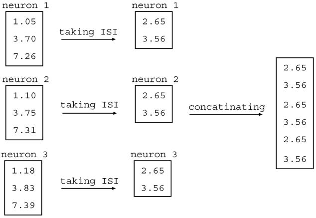
In this paper, the second test statistic is obtained by merging all the spike trains into a single train, taking the interspike intervals (Fig. 5), and applying bzip2 to them. When we use this type of representation, the compressed file obtained from the original set of spike trains will be smaller than those of rate coding surrogates when there are some repeated patterns of spatio-temporal spikes (see Fig. 5). Repeated spatio-temporal patterns look similar in the series of interspike intervals obtained after the process of merging, and thus have similar expressions as well in the ASCII code. Thus the original spike trains are compressed better than their rate coding surrogates.
Fig. 5.

The processes of merging and taking interspike intervals (ISI) for obtaining the second test statistic based on the compression ratio. If there are some repeated patterns of spatio-temporal spikes, then we can also find repeated patterns in the resulting interspike intervals. These parts help to make the compressed file smaller. In the above example, (1.05,1.10,1.18), (3.70,3.75,3.83), and (7.26,7.31,7.39) show repeated firing patterns: spikes in the second and third neurons are delayed from the ones in the first neuron by 0.05 and 0.13, respectively. After merging and taking ISI, this pattern can be seen as repeats of 0.05 followed by 0.08. These repeats make the compressed file smaller.
Since all the test statistics are expected to be smaller for the original spike train if temporal coding is used, we used a one-sided test for statistical significance.
Results
To test the proposed method, artificial data were generated in which only rate coding was present, or in which temporal structure related to the precise timing of spikes was present. Surrogates were then generated according to the procedure detailed in the Methods section, and the two test statistics were calculated for the artificial and surrogate data to determine whether the surrogate method could correctly detect instances of temporal coding or not. Following these tests, the surrogate method was further demonstrated by applying it to real neurophysiological data.
Control: artificial spike trains based on rate coding only (null-hypothesis true)
Spike trains that only used population rate coding were prepared as follows. Ten spike trains were generated that each contained 200 spikes. Each spike time was drawn randomly according to a spike density distribution that was proportional to (0.5 sin(2πt) + 1), where t goes from 0 to 10. Thus the short-term ensemble firing rate (Shadlen and Newsome, 1998) with bins of 0.05 unit time is a noisy sine curve (Fig. 6).
Fig. 6.
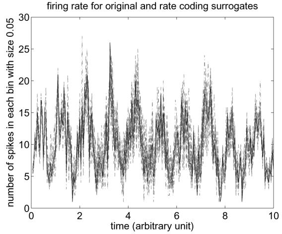
Short-term ensemble firing rates for the original set of spike trains (black solid line) and sets of rate coding surrogates (gray broken lines), in the case of population rate coding.
For the original set of spike trains, 19 sets of rate coding surrogates were generated. Here τ = 0.05 was chosen because we assumed that the time scale of population rate coding, or rate covariance, is about 0.05 s based on Shadlen and Newsome (1998), and that it is equal to or shorter than the mean inter-spike interval of a single neuron. In what follows, we used τ = 0.05 for most cases for the same reason.
The obtained rate coding surrogates preserved the sine curve well, and thus they preserved the information encoded in the local average firing rates of the spike trains (Fig. 6). The two test statistics were calculated for the original set of spike trains and compared with those of rate coding surrogates. The results are summarized in Fig. 7. In this and subsequent figures, the histogram bars show the distribution of the test statistics obtained from the 19 sets of rate coding surrogates, and the vertical line corresponds to the statistic's value for the set of the original spike trains. For each test statistic, comparison of the value for the original spike train set to those of the rate coding surrogates demonstrated that there was no significant difference between the original data and the surrogate population (p > 0.85 and 0.40 for prediction error and compression ratio statistics, respectively). Thus, the results of this control test indicate that the method behaved correctly in that it did not falsely reject the null-hypothesis of population rate coding only.
Fig. 7.

Comparisons between the original set of spike trains and those of rate coding surrogates for the population rate coding case in Fig. 6. Panel (a) shows the values of the prediction error statistic (statistic 1) and panel (b), the values of the compression ratio statistic (statistic 2). In this figure and succeeding ones, the histogram shows the distribution for the test statistics obtained from the set of rate coding surrogates, and the solid line corresponds to the test statistic for the set of the original spike trains. The p-values for (a) and (b) are more than 0.85 and 0.40, respectively.
Synchronous spikes (null-hypothesis is false)
Our second example is the case of synchronous spikes, in which, in contrast to the first example, the temporal structure of the spike trains does contain encoded information (i.e., the precise times of the spikes are critical), but in which there is no regular modulation of the firing rate. Ten identical spike trains were generated such that each had 100 spikes during the time period between 0 and 10. The spike times were determined by a random drawing using a uniform probability distribution between 0 and 10. Given that population rate coding is our null-hypothesis, we generated 19 sets of rate coding surrogates with the bin size τ = 0.05 for the set of spike trains. The original set of spike trains and those of rate coding surrogates were then compared using the two test statistics. The results are shown in Figs. 8(a) and 8(d). The p-values for the first and second test statistics are both less than 0.05. Thus we can rightly reject the null-hypothesis and are led to the correct conclusion that the original spike trains employed temporal coding of information.
Fig. 8.

Comparisons between the original set of spike trains and those of rate coding surrogates for a set of ideally synchronous spike trains ((a) and (d))), a set of synchronous spike trains contaminated by jitter ((b) and (e)), and a set of spike trains synchronized with delays ((c) and (f)). Panels (a)–(c) show the results of using the prediction error statistic (statistic 1) and panels (d)–(f) show the results of using the compression ratio statistic (statistic 2). The p-values for all above cases are less than 0.05.
To test the robustness of the method for uncovering temporal structure even in the presence of some random noise, jitter was added to the spike trains. When the jitter was of a moderate size, both test statistics rejected correctly the null-hypothesis that the spike trains were using only population rate coding. Specifically, Gaussian noise of mean 0 and standard deviation 0.01 was added to all spikes of the 10 spike trains with synchronized spikes described in the preceding paragraph. During the process, spikes that ended up outside of 0-10 interval after addition of the jitter were removed. Then for the noisy spike trains, 19 sets of rate coding surrogates were generated for comparison (Figs. 8(b) and 8(e)). Similar to the noiseless case, the p-values for both test statistics were less than 0.05.
Next, we tested the case where spikes are synchronized with delays (i.e., spikes of one train are shifted by a constant amount from another train.). A master spike train was generated in which spike times were determined by a random drawing using a uniform probability distribution as was done above, except that the range was 0 and 11, in this case. To obtain each spike train, a random number between 0 and 1 was chosen based on a uniform distribution and then subtracted from spike times in the master spike train. The spikes between 0 and 10 for each of these new trains comprised the spike trains used for analysis. As before, for the set of spike trains, 19 sets of rate coding surrogates were generated, and then the original set of ‘synchronized with delays’ spike trains was compared with their corresponding sets of rate coding surrogates (Figs. 8(c) and 8(f)).
Once more a significant difference was found between the original set and those of rate coding surrogates for both test statistics. Therefore, even for the delayed synchrony condition, the proposed method correctly identified the presence of temporal coding in the spike trains.
In sum, these three numerical examples demonstrate that spike trains employing synchrony codes can be correctly detected using the rate coding surrogates.
Cortical songs (null-hypothesis false)
Our third example is cortical songs (Ikegaya et al., 2004). Ikegaya et al. (2004) observed that spontaneous patterns of synaptic inputs are repeated in the same sequential order with millisecond precision in cortical neurons under both in vivo and in vitro conditions. These repeated spatio-temporal patterns of synaptic activity are referred to as cortical songs and are thought to reflect repetitions of spike sequences in the inputs to cortical neurons. When cortical songs exist, the spike trains have temporal-coding aspects. A precisely repeated pattern of spike sequences, such as occurs with cortical songs, would produce repetitions of the same pattern of interspike intervals. Thus the test statistics for the original set of spike trains should be smaller than those for rate coding surrogates in this case.
To test this expectation, 10 cortical-song-like spike trains were prepared in the following way: First, a set of templates was made such that each template comprised 10 spikes over a time period of 0 to π/3. Each spike time was drawn from the uniform distribution between 0 and π/3. Each template was then used to create one spike train of the set by taking the spike pattern of the template and repeating it 10 times. The total duration of each spike train was then cropped to the period 0 to 10.
Here the null-hypothesis is that the cortical-song-like spike trains are based only on the population rate coding. For the spike train set, 19 sets of rate coding surrogates were generated with bin size τ = 0.05. Then the original set of spike trains was compared with those of rate coding surrogates using the two test statistics. The results are shown in Figs. 9(a) and 9(c). Both test statistics correctly rejected the null-hypothesis, implying that they are sensitive to the repeated patterns of interspike intervals in these spike trains.
Fig. 9.

Comparisons between the original set of spike trains and those of rate coding surrogates for ideal cortical songs ((a) and (c)) and jittered cortical songs case ((b) and (d)). Panels (a) and (b) show the results of using the prediction error statistic (statistic 1), and panels (c) and (d) show the results of using the compression ratio statistic (statistic 2). The p-values for all above cases are less than 0.05.
Noise was then added to each spike to test the robustness of the method. For each spike of noise-free spike trains used above, we added jitter that followed a uniform distribution of mean 0 and width 0.001. Then the spikes that were out of the interval between time 0 and 10 were eliminated. The comparison between the original set of noisy cortical-song-like spike trains and those of rate coding surrogates is shown in Figs. 9(b) and 9(d). Once again the null-hypothesis of population rate coding was correctly rejected by both test statistics.
Cricket data
Having tested the surrogate method on simulated data, we now apply it to real data recorded from a cricket wind receptor cell (Suzuki et al., 2000). In this experiment, the abdomen of a cricket was placed in a wind tunnel, which was driven by a Rössler chaos signal delivered by one speaker at each end of the tunnel, and the response of a wind receptor cell was measured. For details of the experiment, see Suzuki et al. (2000).
For the spike train, we generated 19 rate coding surrogates with the bin size of τ = 0.05 s, and compared the wind receptor response to its surrogates using both test statistics (Figs. 10(a) and 10(c)). Both test statistics rejected the null-hypothesis of rate coding only, which leads to the conclusion that the content of the wind receptor spike train employs some form of non-rate coding. This result agrees with the conclusion of Suzuki et al. (2000).
Fig. 10.

Comparisons between the set of original spike trains (solid line) and rate coding surrogates (histogram) for cricket data (Suzuki et al., 2000) ((a) and (c)) and olivocerebellar system data (Blenkinsop and Lang, 2006) ((b) and (d)). Panels (a) and (b) are the results of using the prediction error statistic (statistic 1) and panels (c) and (d), the results of using the compression ratio statistic (statistic 2). The p-value for (b) is more than 0.05, while the p-values for the other cases are less than 0.05.
Olivocerebellar system of rat
Next, we applied the proposed method to data recorded from the rat olivocerebellar system (For a detailed description of experimental data, see Blenkinsop and Lang (2006)). The data set tested here consisted of complex spikes recorded from 36 individual Purkinje cells simultaneously in a ketamine-xylazine anesthetized rat. Only the first 100 seconds of the data set were used. For the spike train set, 19 sets of rate coding surrogates were generated using the bins of size τ = 0.05s. We used τ = 0.05 s since we are interested in population rate coding, which is generally on the order of 0.05 s (Shadlen and Newsome, 1998).
The original set of spike trains and those of rate coding surrogates are compared in Figs. 10(b) and 10(d), which show that the null-hypothesis of population rate coding was rejected when using the second test statistic (the compression ratio). This suggests that the dataset contains information encoded using non-rate coding schemes. These results are consistent with previous physiological studies, which have shown significant levels of synchronization among Purkinje cells (Welsh et al., 1995; Lang et al., 1999; Blenkinsop and Lang, 2006). In this example, the first test statistic, the prediction error, did not reject the null-hypothesis since it cannot extract the information that spreads over more than 5 interspike intervals. This reasoning applies to a general case.
Possibility for simultaneous coding
Lastly, we applied our method to the dual-coding network model of Masuda and Aihara (2002). This network contains two layers. The sensory layer receives common input from a chaotic system and the cortical layer receives its input from the sensory layer. Masuda and Aihara (2002) varied the noise level of neurons in the cortical layer and examined their behavior. When the noise level was low, the cortical layer of the network operated as a temporal coder with synchronous firing, whereas when the noise level was high, it functioned as a poorly performing rate coder. When the noise level was intermediate, the network employed rate coding and performed its best.
To generate spike train data to be tested, the model was run for a sufficient time so that the transient states died away, and then for an additional 10s from which spike activity was used to create 30 spike trains from the cortical layer neurons. We used the same parameter set as Masuda and Aihara (2002) did for generating their Fig. 3(a). Then we tested whether we can correctly identify the rate coding case from others in the following way: For each case, we generated 19 sets of rate coding surrogates for the set of spike trains with the bin size τ = 0.05 s. Then the original set of spike trains was compared with those of rate coding surrogates using the second test statistic, the compression ratio statistic. Here we only used the compression ratio statistic since the example of olivocerebellar system showed that the compression ratio has the stronger power of detection than the first test statistic (the prediction error).
The results are compared in Fig. 11. When there was no noise present (σ = 0), the null-hypothesis of rate coding only was correctly rejected (Fig. 11(a)). When a large amount of noise was added (σ = 0.02), the null-hypothesis was not rejected (Fig. 11(c)). These results agree with our expectation and the previous findings. When the intermediate-size noise was added (σ = 0.005), the null-hypothesis was rejected (Fig. 11(b)), suggesting that some form of temporal coding was present. This implies that there are still significantly more synchronous spikes than expected by chance under the intermediate-size noise.
Fig. 11.

Comparisons between the original set of spike trains and those of rate coding surrogates with the dual-coding model of Masuda and Aihara (2002). In these figures, we used 0.05 s for τ. Panel (a) is the case without noise (σ = 0), panel (b) is the case with intermediate-size noise (σ = 0.005), and panel (c) is the case with large noise (σ = 0.02). All panels are obtained by using the compression ratio statistic. Here σ is the standard deviation of the Gaussian noise defined in Masuda and Aihara (2002). The p-value for (c) is more than 0.95, while the p-values for the other cases are less than 0.05.
Before accepting this conclusion, however, we consider the possibility that the time scale for the population rate coding is shorter than 0.05s. To test this possibility, τ was reduced to 0.01s, and the analysis was repeated. Similar results were obtained (Fig. 12), supporting the original suggestion that temporal coding was present under the intermediate-size noise.
Fig. 12.

Comparisons between the original set of spike trains and those of rate coding surrogates with the dual-coding model of Masuda and Aihara (2002). All parameters and tests are the same as in Fig. 11 except that here τ = 0.01s. The p-values for (c) is more than 0.90, while the p-values for the other cases are less than 0.05.
According to Masuda and Aihara (2002), this intermediate-size noise case is one where population rate coding is most effective. However, although rate coding is effective, it appears that the network still uses temporal coding to some extent. Therefore, these results indicate the possibility that temporal and rate coding can both be used in a single neural network simultaneously to improve its efficiency. We call this situation simultaneous coding (Masuda, 2006). Some prior experimental (Riehle et al, 1997; Huxter et al., 2003; Friedrich et al., 2004) and theoretical (Masuda, 2006) reports suggest that the firing rate and synchrony can encode different types of information, which is one reason for why a network would employ simultaneous coding.
Discussion
In this paper, we have proposed an algorithm for generating surrogate data of spike trains, or rate coding surrogates. The surrogate data are generated so as to preserve the distribution of interspike intervals perfectly and the short-term average firing rates in bins approximately. Therefore, these surrogates can be used for constructing hypothesis testing related to whether or not only rate coding is being used by neurons or neuronal populations. We also described two test statistics for detecting the difference between the original data and rate coding surrogates: the first test statistic is based on prediction using nearest neighbors; the second test statistic is the compression ratio of interspike intervals. The compression ratio statistic is more powerful than the prediction error statistic since there is no assumption on how future spike times depend on past ones. Although we used bzip2 for obtaining the second test statistic, other compression algorithms can be used instead, and might be more applicable depending on the specific coding schemes that are suspected.
Number of surrogate data
We used 19 sets of surrogates for the 5% confidence level since when the original dataset follows the null-hypothesis, one needs 1/α − 1 surrogates so that the original dataset yields the smallest value of the statistic among the original dataset and its surrogates with probability by chance (Kantz and Schreiber, 1997). In practice, 19 was also enough for getting consistent results. We repeated the same calculations for obtaining Fig. 10 for 9 more times. Then, as for the cricket data, the 5% point of the compression ratio statistic was distributed in [0.1810, 0.1827]. Therefore, we obtained rejections for all 10 times. As for inferior olive data, the 5% point of the compression ratio statistic was distributed in [0.0808, 0.0811]. Hence, from all 10 trials, we had rejections.
Choice of bin width τ
The bin width τ should be chosen based on the timescale for the assumed rate coding. In this paper, we took the value from Shadlen and Newsome (1998) and set τ = 0.05 (s) for most analyses. However, to investigate the sensitivity of the results to the choice of τ, we repeated the analysis for some of the examples presented in the Results section using values of τ that were one order of magnitude greater or smaller than the standard value of τ(=0.05) that was generally used through out the rest of the paper (see Figs. 13 and 14 for the cases of τ = 0.005(s) and τ = 0.5(s), respectively; also compare Figs. 11 and 12). The results shown in Figs. 13 and 14 suggest that the obtained results using surrogate data are relatively insensitive to the specific value of the bin width τ.
Fig. 13.

Dependence of results on choice of τ. Most of the analysis so far used a τ of 0.05s. This figure shows the results of the analysis using a τ = 0.005s for selected datasets. The compression ratio statistic was used for all panels. Panels (a), (b), (c), (d), and (e) correspond to the datasets of rate coding, clean synchrony, clean cortical songs, cricket, and olivecerebellar system, respectively. For producing (e), the first 20 seconds of the data were used.
Fig. 14.

Dependence of results on choice of τ. The same as Fig. 13 except that here τ = 0.5s. Also, in panel (e), the first 100 seconds of the dataset were used.
By changing τ, we might be able to evaluate the precision of temporal coding.
Other possible alternatives
Three other possible alternative methods for generating spike train surrogates that preserve the short-term average firing rate have been described previously. The first is adding jitter to each spike (Bialek et al., 1991; Reinagel and Reid, 2000; Gerstein, 2004), the second involves using a time-varying model (Poisson or non-Poisson) (van Steveninck et al., 1997; Reinagel and Reid, 2000; Ventura et al., 2002, 2005), and the third is to use multiple trials (Pipa et al., 2003; Pipa and Grün, 2003). However, each of these has significant disadvantages. By adding jitter to the spikes, the distribution of interspike intervals is changed, which may cause a spurious rejection or weaken the discrimination power of the statistical tests, because it is not a constrained realization (Theiler and Prichard, 1996). In the case of a time varying model, estimation of the time varying parameters is difficult and problematic. For example, if a Poisson process is used as the underlying model, then that requires the assumption that interspike intervals have an exponential distribution. This assumption is too strong and not strictly correct because of refractory periods of neurons. In the case of using a multiple trials approach, datasets need to have multiple trials, which assumes event-related responses and thus is not always possible, for example, in the case of spontaneous activity.
Therefore, compared with the other potential approaches, the proposed method of rate coding surrogates has three advantages. The first is that no underlying model is assumed. Second, we need not fit any parameters that may cause spurious rejections. Third, by choosing τ properly, we can cover situations from the rate coding for a single neuron to the population rate coding (Shadlen and Newsome, 1998; Mar et al., 1999; van Rossum et al., 2002).
In sum, although there are some interesting works that have characterized aspects of temporal coding schemes (Bialek et al., 1991; van Steveninck et al., 1997; Strong et al., 1998; Reinagel and Reid, 2000; Gerstein, 2004; Ventura et al., 2002, 2005; Pipa et al., 2003; Pipa and Grün, 2003; Panzeri and Schultz, 2001), there has been no published work, as far as the authors know, that constructs hypothesis testing with explicit surrogates by preserving the distribution of interspike intervals completely for this purpose. Recently, we learned that Denker et al. (2005) also used a technique similar to ours for detecting phase locking in spike trains. In their method, interspike intervals were exchanged locally. For their purpose, this local exchange was appropriate because their goal was simply to preserve the temporal change of distribution for interspike intervals. However, to test the rate coding hypothesis, it is necessary to exchange interspike intervals globally because the temporal change of interspike interval distribution may convey the information and we want to separate it from the rate coding.
Implications of results
Application of the proposed method to the cricket data showed that information in the cricket dataset is not based on rate coding only. Similarly, for the olivocerebellar data, the proposed method detected the presence of temporal coding, strengthening prior conclusions on the importance of synchronization in the olivocerebellar system (Lang et al., 1999). We have also pointed out the possibility of the simultaneous coding, under which the short-term average firing rate and spike times are used simultaneously for coding the information. We have demonstrated the ability of the method to detect such simultaneous coding of information. Given the complexity of neuronal codes and possibility of multiple codes being used, the rate coding surrogates method described here represents a potentially powerful tool for guiding analysis of spike train data, particularly that from large neuronal ensembles.
Acknowledgments
This research is partially supported by Grant-in-Aid for Scientific Research on Priority Areas —Higher-Order Brain Functions—(17022012), the Advanced and Innovational Research program in Life Sciences from MEXT of Japan, NIAAA(AA016566), and NINDS (NS037028).
Footnotes
Publisher's Disclaimer: This is a PDF file of an unedited manuscript that has been accepted for publication. As a service to our customers we are providing this early version of the manuscript. The manuscript will undergo copyediting, typesetting, and review of the resulting proof before it is published in its final citable form. Please note that during the production process errors may be discovered which could affect the content, and all legal disclaimers that apply to the journal pertain.
References
- Abeles M. Corticonics. Cambridge University Press; Cambridge, UK: 1991. [Google Scholar]
- Araki O, Aihara K. Dual information representation with stable firing rates and chaotic spatiotemporal spike patterns in a neural network model. Neural Comp. 2001;13(12):2799–822. doi: 10.1162/089976601317098538. [DOI] [PubMed] [Google Scholar]
- Bialek W, Rieke F, van Steveninck RRD, Warland D. Reading a neural code. Science. 1991;252(5014):1854–7. doi: 10.1126/science.2063199. [DOI] [PubMed] [Google Scholar]
- Blenkinsop TA, Lang EJ. Block of inferior olive gap junctional coupling decreases Purkinje cell complex spike synchrony and rhythmicity. J Neurosci. 2006;26(6):1739–48. doi: 10.1523/JNEUROSCI.3677-05.2006. [DOI] [PMC free article] [PubMed] [Google Scholar]
- Bryant HK, Segundo JP. Spike initiation by transmembrane current: white-noise analysis. J Physiol London. 1976;260(2):279–314. doi: 10.1113/jphysiol.1976.sp011516. [DOI] [PMC free article] [PubMed] [Google Scholar]
- Cilibrasi R, Vitanyi P. Clustering by Compression. IEEE T Inform Theory. 2005;51(4):1523–45. [Google Scholar]
- Denker M, Timme M, Roux S, Riehle A, Grün S. Society for Neuroscience. Washington D.C.: 2005. Detecting transient temporal relationships between spikes and LFP by phase analysis. Abstract Viewer/Itinerary Planner, Program No. 970.10. [Google Scholar]
- Friedrich RW, Habermann CJ, Laurent G. Multiplexing using synchrony in the zebrafish olfactory bulb. Nat Neurosci. 2004;7(8):862–71. doi: 10.1038/nn1292. [DOI] [PubMed] [Google Scholar]
- Gersenfeld N. The nature of mathematical modeling. Cambridge University Press; Cambridge, UK: 1999. [Google Scholar]
- Gerstein GL. Searching for significance in spatio-temporal firing patterns. Acta Neurobiol Exp. 2004;64(4):203–7. doi: 10.55782/ane-2004-1506. [DOI] [PubMed] [Google Scholar]
- Huxter J, Burgess N, O'Keefe J. Independent rate and temporal coding in hippocampal pyramidal cells. Nature. 2003;425(6960):828–32. doi: 10.1038/nature02058. [DOI] [PMC free article] [PubMed] [Google Scholar]
- Ikegaya Y, Aaron G, Cossart R, Aronov D, Lampl I, Ferster D, Yuste R. Synfire chains and cortical songs: temporal modules of cortical activity. Science. 2004;304(5670):559–64. doi: 10.1126/science.1093173. [DOI] [PubMed] [Google Scholar]
- Kantz H, Schreiber T. Nonlinear Time Series Analysis. Cambridge University Press; Cambridge, UK: 1997. [Google Scholar]
- Lang EJ, Sugihara I, Welsh JP, Llinás R. Patterns of spontaneous Purkinje cell complex spike activity in the awake rat. J Neurosci. 1999;19(7):2728–39. doi: 10.1523/JNEUROSCI.19-07-02728.1999. [DOI] [PMC free article] [PubMed] [Google Scholar]
- Lu T, Liang L, Wang X. Temporal and rate representations of time-varying signals in the auditory cortex of awake primates. Nat Neurosci. 2001;4(11):1131–8. doi: 10.1038/nn737. [DOI] [PubMed] [Google Scholar]
- MacLeod K, Bäcker A, Laurent G. Who reads temporal information contained across synchronized and oscillatory spike trains? Nature. 1998;395(6703):693–8. doi: 10.1038/27201. [DOI] [PubMed] [Google Scholar]
- Mainen ZF, Sejnowski TJ. Reliability of spike timing in neocortical neurons. Science. 1995;268(5216):1503–6. doi: 10.1126/science.7770778. [DOI] [PubMed] [Google Scholar]
- Mar DJ, Chow CC, Gerstner W, Adams RW, Collins JJ. Noise shaping in populations of coupled model neurons. Proc Natl Acad Sci USA. 1999;96(18):10450–5. doi: 10.1073/pnas.96.18.10450. [DOI] [PMC free article] [PubMed] [Google Scholar]
- Masuda N, Aihara K. Bridging rate coding and temporal spike coding by effect of noise. Phys Rev Lett. 2002;88(24):248101. doi: 10.1103/PhysRevLett.88.248101. [DOI] [PubMed] [Google Scholar]
- Masuda N, Aihara K. Duality of rate coding and temporal coding in multilayered feedforward networks. Neural Comp. 2003;15(1):103–25. doi: 10.1162/089976603321043711. [DOI] [PubMed] [Google Scholar]
- Masuda N, Aihara K. Dual coding and effects of global feedback in multilayered neural networks. Neurocomputing. 2004;58:33–9. [Google Scholar]
- Masuda N. Simultaneous rate-synchrony codes in populations of spiking neurons. Neural Comp. 2006;18(1):45–59. doi: 10.1162/089976606774841521. [DOI] [PubMed] [Google Scholar]
- Panzeri S, Schultz SR. A unified approach to the study of temporal, correlational, and rate coding. Neural Comp. 2001;13(6):1311–49. doi: 10.1162/08997660152002870. [DOI] [PubMed] [Google Scholar]
- Pipa G, Diesmann M, Grün S. Significance of joint-spike events based on trial-shuffling by efficient combinatorial methods. Complexity. 2003;8(4):79–86. [Google Scholar]
- Pipa G, Grün S. Non-parametric significance estimation of joint-spike events by shuffling and resampling. Neurocompting. 2003;52-4:31–7. [Google Scholar]
- Perkel DH, Bullock TH. Neural coding. Neurosciences Res Prog Bull. 1968;6(3):221–348. [Google Scholar]
- Press WH, Teukolsky SA, Vetterling WT, Flannery BP. Numerical Recipes in C. Cambridge University Press; Cambridge, UK: 1988. [Google Scholar]
- Reinagel P, Reid RC. Temporal coding of visual information in the thalamus. J Neurosci. 2000;20(14):5392–400. doi: 10.1523/JNEUROSCI.20-14-05392.2000. [DOI] [PMC free article] [PubMed] [Google Scholar]
- Riehle A, Grün S, Diesmann M, Aertsen A. Spike synchronization and rate modulation differentially involved in motor cortical function. Science. 1997;278(5345):1950–3. doi: 10.1126/science.278.5345.1950. [DOI] [PubMed] [Google Scholar]
- Scheinkman JA, LeBaron B. Nonlinear dynamics and stock returns. J Business. 1989;62(3):311–37. [Google Scholar]
- Schreiber T, Schmitz A. Improved surrogate data for nonlinear tests. Phys Rev Lett. 1996;77(4):635–38. doi: 10.1103/PhysRevLett.77.635. [DOI] [PubMed] [Google Scholar]
- Schreiber T. Constrained randomization of time series data. Phys Rev Lett. 1998;80(10):2105–8. [Google Scholar]
- Shadlen MN, Newsome WT. The variable discharge of cortical neurons: implications for connectivity, computation, and information coding. J Neurosci. 1998;18(10):3870–96. doi: 10.1523/JNEUROSCI.18-10-03870.1998. [DOI] [PMC free article] [PubMed] [Google Scholar]
- Small M, Yu D, Harrison RG. Surrogate test for pseudoperiodic time series. Phys Rev Lett. 2001;87(18):188101. [Google Scholar]
- Strong SP, Koberle R, van Steveninck RRD, Bialek W. Entropy and information in neural spike trains. Phys Rev Lett. 1998;80(1):197–200. [Google Scholar]
- Suzuki H, Aihara K, Murakami J, Shimozawa T. Analysis of neural spike trains with interspike interval reconstruction. Biol Cyber. 2000;82(4):305–11. doi: 10.1007/s004220050584. [DOI] [PubMed] [Google Scholar]
- Theiler J, Eubank S, Longtin A, Galdrikian B, Farmer JD. Testing for nonlinearity in time-series: the method of surrogate data. Physica D. 2000;58(14):77–94. [Google Scholar]
- Theiler J, Prichard D. Constrained-realization Monte-Carlo method for hypothesis testing. Physica D. 1996;94(4):221–35. [Google Scholar]
- Tiesinga PHE, Fellis JM, José JV, Sejnowski TJ. Information transfer in entrained cortical neurons. Network. 2002;13(1):41–66. [PubMed] [Google Scholar]
- Thorpe S, Fize D, Marlot C. Speed of processing in the human visual system. Nature. 1996;381(6582):520–22. doi: 10.1038/381520a0. [DOI] [PubMed] [Google Scholar]
- van Rossum MCW, Turrigiano GG, Nelson SB. Fast propagation of firing rates through layered networks of noisy neurons. J Neurosci. 2002;22(5):1956–66. doi: 10.1523/JNEUROSCI.22-05-01956.2002. [DOI] [PMC free article] [PubMed] [Google Scholar]
- van Steveninck RRD, Lewen GD, Strong SP, Koberle R, Bialek W. Reproducibility and variability in neural spike trains. Science. 1997;275(5307):1805–8. doi: 10.1126/science.275.5307.1805. [DOI] [PubMed] [Google Scholar]
- Ventura V, Carta R, Kass RE, Gettner SN, Olson CR. Statistical analysis of temporal evolution in single-neuron firing rates. Biostatistics. 2002;3(1):1–20. doi: 10.1093/biostatistics/3.1.1. [DOI] [PubMed] [Google Scholar]
- Ventura V, Cai C, Kass RE. Statistical assessment of time-varying dependency between two neurons. J Neurophysiol. 2005;94(4):2940–7. doi: 10.1152/jn.00645.2004. [DOI] [PubMed] [Google Scholar]
- Welsh JP, Lang EJ, Sugihara I, Llinás R. Dynamic organization of motor control within the olivocerebellar system. Nature. 1995;374(6521):453–7. doi: 10.1038/374453a0. [DOI] [PubMed] [Google Scholar]