Preservation of Spectrotemporal Tuning Between the Nucleus Laminaris and the Inferior Colliculus of the Barn Owl

Abstract

Performing sound recognition is a task that requires an encoding of the time-varying spectral structure of the auditory stimulus. Similarly, computation of the interaural time difference (ITD) requires knowledge of the precise timing of the stimulus. Consistent with this, low-level nuclei of birds and mammals implicated in ITD processing encode the ongoing phase of a stimulus. However, the brain areas that follow the binaural convergence for the computation of ITD show a reduced capacity for phase locking. In addition, we have shown that in the barn owl there is a pooling of ITD-responsive neurons to improve the reliability of ITD coding. Here we demonstrate that despite two stages of convergence and an effective loss of phase information, the auditory system of the anesthetized barn owl displays a graceful transition to an envelope coding that preserves the spectrotemporal information throughout the ITD pathway to the neurons of the core of the central nucleus of the inferior colliculus.

INTRODUCTION

There is considerable evidence that the time-dependent structure of auditory signals is a major factor in the task of sound recognition. Fine temporal structure is a significant determinant in the discrimination and recognition of birds’ songs (Brenowitz 1983) and evidence suggests that intact temporal information permits the comprehension of human speech even with degraded spectral cues (Drullman et al. 1994; Shannon et al. 1995; Wright et al. 1997). To process this information, the brain must encode the spectral properties of the stimulus as a function of time.

It is known that the owl is capable of discriminating between nearby frequencies with ease (Quine and Konishi 1974) and between complex noises that differ by as little as 2.5 dB in a single 1/3 octave band (Konishi and Kenuk 1975), but the stimuli used in these studies were not characterized in terms of their instantaneous frequency structure. Nonetheless, behavior suggests that the owl is capable of subtle tasks of recognition: for example, the owl has been reported to be able to distinguish between the sounds of a mouse walking through dry leaves versus a mouse walking through chopped-up paper (Konishi and Kenuk 1975). Combined with the psychophysical work in humans on the relevant stimulus parameters for sound recognition, it is likely that the owl is capable of detecting spectrotemporal information on a relatively short timescale.

The brain stem auditory nuclei of the barn owl have been primarily characterized in terms of their responses to the two major binaural cues for sound localization: the interaural time difference (ITD) and the interaural level difference (ILD). However, all auditory information, including that needed for sound recognition and discrimination, ascends through these nuclei. Keller and Takahashi (2000) characterized the spectrotemporal tuning—i.e., the joint distribution over instantaneous frequency and time of the stimuli preceding spikes (Klein et al. 2000)—of the neurons in the lateral shell of the central nucleus of the inferior colliculus (ICls). ICls receives inputs from both the ITD pathway [by the core of the central nucleus of the inferior colliculus (ICcc); Takahashi and Konishi 1988] and the ILD pathway [by nucleus angularis (NA) and the nucleus dorsal lemnisci lateralis pars posterior (LLDp); Takahashi et al. 1989].

Neurons in the initial stages of the ITD processing pathway of the barn owl, including the auditory nerve, nucleus magnocellularis (NM), and nucleus laminaris (NL), are known to phase lock to and thus to convey spectral information for frequencies as high as 8 kHz (Carr and Konishi 1990; Köppl 1997; Peña et al. 1996; Sullivan and Konishi 1984); phase locking was also shown in ITD-related neurons in mammalian systems (de Boer and de Jongh 1978; Eggermont 1993; Kim and Young 1994; Lewis et al. 2002; Louage et al. 2004). In previous work (Christianson and Peña 2006) we showed that the transition from NL to ICcc includes a convergence across units with similar tuning to optimize the information on ITD conveyed by the firing rates of single neurons. Additionally, the time required for an owl to estimate the ITD of a signal (Konishi 1973) and the temporal resolution with which human subjects can follow moving auditory stimuli (Grantham and Wightman 1978) are both on the order of tens of milliseconds. Taken together, this suggests that the computation of ITD involves sufficient pooling across time or population that the neurons of ICcc may show a temporal resolution only on the order of tens of milliseconds; consistent with this, there are no reports of phase locking in the ICcc of owls. This would suggest that the observed envelope coding in the ICls (Keller and Takahashi 2000) would come from the ILD pathway.

In this study, we analyze the spectrotemporal receptive properties of NL, the locus of the computation of ITD, and ICcc, the terminus of the ITD pathway. We show that throughout this pathway the reliability in response to the time-varying spectrum of the stimulus is maintained despite the loss of phase information for high frequencies. Thus the reduction of noise from NL to ICcc previously described (Christianson and Peña 2006) and the loss of phase locking do not come at the expense of the representation of spectrotemporal cues and, in fact, maintain a millisecond-resolution envelope code of the stimulus spectrum.

METHODS

Data were obtained from 16 adult barn owls (Tyto alba) of both sexes bred in captivity. Owls were anesthetized by intramuscular injection of ketamine hydrochloride (20 mg/kg, Ketaject, Phoenix Pharmaceuticals, Mountain View, CA) and xylazine (2 mg/kg, Xyla-Ject, Phoenix Pharmaceuticals). An adequate level of anesthesia was maintained by additional injections of both when needed. During the first recording session, ear bars and beak holder were used to position the owl’s head with the beak rotated in the sagittal plane (30° for the ICcc recording and 70 for NL). A head plate was implanted by removing the top layer of the skull and fixed with dental cement. A stainless steel reference post was implanted posterior to the head plate and similarly fixed with dental cement. Once the head plate was implanted, the ear bars and beak holder were removed and the head plate was used to hold the head in position from that point forward and in all following recording sessions. A craniotomy was made over the recording site. The craniotomy was packed with gelfoam and sealed with dental cement and the scalp was sutured at the end of the session. After the surgery, analgesics (Ketoprofen, 10 mg/kg, Ketofen, Merial) were administered. The protocol for this study followed the National Institutes of Health Guide for the Care and Use of Laboratory Animals and was approved by the Institute’s Animal Care and Use Committee.

Electrophysiology

We positioned the recording electrodes by known stereotaxic coordinates and by the units’ response properties, using white noise and tones of manually set ITD and frequency as search stimuli. NL is easily identified by the large field potentials (called neurophonics) that vary in amplitude with ITD; ICcc neurons were distinguished by the presence of ITD sensitivity without side-peak suppression and by an absence of tuning to interaural level differences. We isolated and maintained NL single neurons by a loose patch method (Peña et al. 1996, 2001) in which the electrode served as a suction electrode, allowing us to hold neurons for a long time. Neural signals were serially amplified by an Axoclamp-2A (Molecular Devices, Palo Alto, CA) and a custom-made AC amplifier (µM-200; B.E.S., California Institute of Technology, CA). ICcc neurons were recorded using tungsten electrodes (A–M Systems, Carlsborg, WA). A spike discriminator (SD1, Tucker-Davis Technologies, Gainesville, FL) converted neural impulses into TTL pulses for an event timer (ET1, Tucker-Davis Technologies), which recorded the timing of the pulses. A computer was used for stimulus synthesis and online data analysis.

It is possible that the differences in the recording techniques used for ICC and NL contributed to the changes observed in response properties. The “loose patch” recording technique was developed to overcome the traditional difficulty in obtaining stable and well-isolated recordings of coincidence detector neurons in NL and in its mammalian equivalent, the medial nucleus of the superior olive (MSO). We consider that the recorded NL neurons were in reasonably good health because we obtained stable recordings lasting for >1 h. During these periods, the neurons showed a high degree of phase locking and stable tuning to ITD. Also, we previously showed that NL neurons recorded by loose patch have tuning to ITD that is tolerant to a broad range of sound intensity (Peña et al. 1996) and precisely matches the values expected by conduction delays of afferent fibers published in previous studies (Carr and Konishi 1990; Peña et al. 2001). We reasoned that if either recording technique was affecting the response properties, the most likely one would be the loose patch because the electrode is presumably attached or very close to the cell’s soma. Therefore a decline in the ability of phase locking should be observed in NL neurons, rather than in ICC. On the other hand, the loose patch technique is not only significantly more time consuming than regular metal electrodes but also more invasive because glass pipettes suitable for patch clamping are used. For these reasons, we refrained from using loose patch for recording ICC units. Although we consider it unlikely, we cannot completely rule out that the use of metal electrodes biased our sample of ICC neurons toward only those that did not show phase locking. An additional bias may have been introduced by our requirement for recording stability. Our full protocol (to collect the data presented both here and elsewhere) required holding a cell for a minimum of about 1 h; this constraint contributed to our relatively low cell counts.

Acoustic stimulation

An earphone assembly consisting of a Knowles 1914 receiver, a Knowles 1743 damping device, and a Knowles 1939 microphone delivered sound stimuli. These components are encased in an aluminum cylinder that fits into the owl’s ear canal. The gaps between the cylinder and the ear canal were filled with silicon impression material (Gold Velvet II, Earmold and Research Laboratory, Wichita, KS). At the beginning of each experimental session, the earphone assemblies were automatically calibrated (Arthur 2004). The computer was programmed to equalize sound pressure level and phase for all frequencies within the frequency range relevant to the experiment for both tonal and broadband stimulation. Noise was designed by specifying the desired amplitude and phase spectrum, applying the calibration, and computing the inverse Fourier transform. Initial phase was randomized while preserving the desired interaural phase difference for each trial.

Tonal and broadband stimuli 100 ms in duration with 5-ms rise/fall times were presented once per second. We used PA4 digital attenuators (Tucker-Davis Technologies) to vary stimulus sound levels. Stimuli were presented at an intensity of 50 dB/SPL, which was found to be consistently above the saturation threshold of rate-intensity responses in both NL and ICcc.

Data collection

Data on the variability and reproducibility of neuronal responses were obtained using a frozen noise protocol, in which a single white noise stimulus (with power between 1,000 Hz and 12 kHz) was repeatedly presented at a sampling rate of 48,077 Hz. To minimize any effects of habituation, two separate and unique frozen noises with different ITDs were randomly interleaved. Rate-ITD functions were obtained by scanning in 30-µs steps from ±2,000 to ±3,000 µs.

The occurrence of a spike is presumably related to the occurrence of a stimulus feature to which the neuron is sensitive. To determine the stimulus features to which the neuron is sensitive we used reverse correlation (de Boer and de Jongh 1978). In this method, we first compute the pre-event stimulus ensemble (PESE): a matrix in which row n contains the segment of the stimulus that preceded spike n. By examining the statistical properties of this matrix it is possible to determine the stimulus features that precede, and presumably elicit, spikes.

Data for reverse correlation were obtained by presenting 100-ms de novo–synthesized broadband signals at the estimated characteristic delay (CD) of each neuron, randomly interleaved with stimuli at a different ITD; stimuli were presented with an interstimulus interval of 500 ms and we attempted to collect between 400 and 800 trials for each ITD condition. Because of the higher reliability in the response to ITD of ICcc neurons (Christianson and Peña 2006), we used the best ITD. In NL, we determined the CD by collecting rate-ITD curves at different frequencies and finding the peak at which all of them overlapped. The window of the reverse correlation (i.e., the amount of stimulus preceding each spike that was considered in the analysis) was 15 ms; manual verification did not indicate that any neurons in our population had a response function whose temporal extent exceeded that limit. To ensure that segments of the interstimulus interval and the rise period of the stimulus were not included in the reverse correlation analysis (or, in other words, to guarantee that the reverse correlation was done on a signal with stationary statistics), spikes that occurred in the 20 ms immediately after stimulus onset were excluded; this exclusion was also sufficient to guarantee that the onset transient was excluded and that the neuron had reached a stable firing rate and we encountered no neurons that had onset-only responses. After this exclusion, a large number of spikes were still left for consideration (average number of spikes used in the reverse correlation analysis per neuron for NL: 4,158 ± 1,818; ICcc: 3,915 ± 1,788).

Analysis

The spike-triggered average (STA) is given by averaging the PESE matrix across columns (spikes), to give the average waveform preceding each spike. When computed with Gaussian white noise, the STA is the best estimate of the linear impulse response function of the neuron (de Boer and de Jongh 1978). However, the STA incorporates the response of the neuron to phase as well as spectral power and, for neurons that do not exhibit phase-locking, the STA will not generate meaningful structure (Eggermont et al. 1983b). The response of a neuron can also be characterized using the spectrotemporal receptive field (STRF), which gives the average spectotemporal distribution of the stimulus preceding each spike (Eggermont et al. 1983b).

An estimate of the reproducibility of response was derived using the shuffled autocorrelogram (SAC) as presented by Joris (2003). We have N spike trains arising from presentations of the same broadband stimulus to a particular neuron and began by choosing the first spike train. For each spike in that train, we computed the forward time intervals (that is, the difference in spike times between that spike and all spikes occurring after it relative to stimulus onset) between that spike and all spikes in the other spike trains, and then this procedure was repeated until all spikes in all spike trains have been used as the reference. Because there are no intra-train comparisons, effects of refractory period are eliminated. The SAC is guaranteed to be symmetric about the delay of zero (each forward time interval will reoccur as a backward time interval), and hence we need only consider the forward time intervals, though reverse intervals are also plotted for visual clarity. A normalizing factor N(N – 1)r²ΔτD, where r is the mean firing rate, Δτ is the bin width of the correlogram, and D is stimulus duration, results in a unity baseline, where a spike train with Poisson statistics will have a flat SAC of height 1. We used a histogram of 50-µs bin width, as in Louage et al. (2004).

To compute the STRF, we used the same procedure as Keller and Takahashi (2000). Each 15-ms-long stimulus segment in the PESE was passed through a gammatone filter bank, with 80 channels spaced linearly between 1 and 10 kHz. The envelope of the stimulus in each channel was extracted using the Hilbert transform, after which the average envelope of the channels across the PESE was computed, giving a phase-insensitive estimate of the average power in each frequency channel preceding spikes. The same process (up to averaging across stimulus samples) was used to compute a spectrogram (spectrotemporal distribution).

Because STRFs are not in general square (they can have different numbers of time and frequency bins), we used the singular value decomposition (SVD) for principal component analysis. In the SVD, an m × n matrix M is represented by M = UΛV^T, where U is m × m, V is n × n, and Λ is an m × n diagonal matrix whose entries are the singular values λ_i of M. The fractional energy of a singular value λ_i, given by ${\mathrm{\lambda }}_i^{\mathit{2}}/{\displaystyle {\sum }_j{\mathrm{\lambda }}_j^{\mathit{2}}}$, is a measure of the relative contribution of the associated singular vector pair to the reconstruction of the overall matrix. The fractional energy of λ₁ is equal to 1 – α_SVD, where α_SVD is the degree of inseparability defined by Depireux et al. (2001).

The spectral tuning was estimated in the STRF using the vector produced by summing the STRF along the time axis. The vector was normalized to have a maximum positive value of 1, with a possibly negative minimum, and was quantified using the frequency corresponding to the maximum positive value in the vector (PF), the width of the peak of the vector at a height of 0.5 (BW_0.5), and the frequency on which BW_0.5 was centered (CF_0.5). The peak time (PT), 0.5 temporal width (TW_0.5), and center time (CT_0.5) were defined analogously but over the time axis instead of the frequency axis.

The STRF was used to predict the response of a neuron to a novel stimulus by convolving each frequency channel in the spectrogram of the stimulus by the corresponding channel in the STRF and then averaging across frequency channels. Comparison was done between the predicted response and the actual poststimulus time histogram (PSTH) of the neuron for frozen noise by computing the correlation coefficient over 80 ms of stimulus. Both PSTH and predicted firing rate were first convolved by a Gaussian kernel with 0.5 ms SD.

In analyzing data that are not normal in distribution, we use the median (denoted by Q₂), which in boxplots is given by the center line; Q₁ and Q₃ are the lower and upper quartiles, respectively, and give the edges of the box. Whiskers give the extent of the data, up to a maximum of 1.5-fold the interquartile range; data points outside this range are treated as outliers and marked individually.

RESULTS

We recorded from 19 NL neurons and 27 ICcc neurons using a reverse correlation protocol of repeated presentations of unique broadband noise stimuli (see METHODS). To compare the spectrotemporal tuning of the two nuclei, we began by determining that phase locking is not present in ICcc neurons for the frequencies we considered. We then analyzed the variability of the response to frozen sound for a subset of these units (10 NL neurons and 22 ICcc neurons) and established that, despite the lack of phase locking, the overall amount of reproducibility of the spike trains was the same in the two nuclei. Consistent with this, in both nuclei we see highly similar spectrotemporal tuning. Finally, using response prediction, we demonstrate that linear estimates of response are equally valid in either nucleus, suggesting that there is no reason to believe that the spectrotemporal response functions are in fact dissimilar.

Phase sensitivity

We began by establishing whether phase sensitivity, which is known to be present in NL neurons in the form of phase-locking (Carr and Konishi 1990; Peña et al. 1996), is preserved in ICcc. The STA is computed by averaging the PESE across spikes and gives the average stimulus preceding a spike and therefore an estimate of the spectral, temporal, and phasic aspects of the tuning of the neuron. For nonfrozen broadband stimuli, the STA shows an organized structure only in the case where there is locking to the fine structure of the stimulus (Eggermont 1993); intuitively, this is because unless the spikes are synchronized to a particular phase of the stimulus, the averaging across the PESE will result in destructive interference comparable to averaging across time. Consistent with reports of phase locking in NL, we saw coherent STAs for all NL neurons examined (Fig. 1, A and B). In contrast, a meaningful STA was never observed in our population of ICcc neurons (Fig. 1, C and D), which is consistent with an elimination of fine structure locking from NL to ICcc. The presence of a coherent white-noise STA is not a direct indication of phase locking to pure tones; in particular, this observation cannot be directly related to the most common measure of phase locking—vector strength—although we suggest that the fact that even our highest-frequency NL neurons (CF of 6.4 kHz) showed a coherent STA sets a ceiling on possible vector strength values in ICcc. On the other hand, because there is evidence that vector strength from tone response does not correctly estimate a neuron’s response to broadband noise (Yin and Chan 1990), the STA is more meaningful in the context of a study using broadband signals. Mammalian data reports a continued phase locking in IC, although at reduced maximum frequencies compared with the earlier nuclei (Liu et al. 2006). The neuron in our data set with the lowest CF₁₀ (1,170 Hz) is shown in Fig. 1D, and did not display any difference compared with higher-frequency units (Fig. 1C has a CF₁₀ of 3,500 Hz). Although we cannot rule out phase locking in ICcc at frequencies <1 kHz, this is a dramatic reduction compared with the ability of NL neurons to phase lock at frequencies >7 kHz.

FIG. 1.

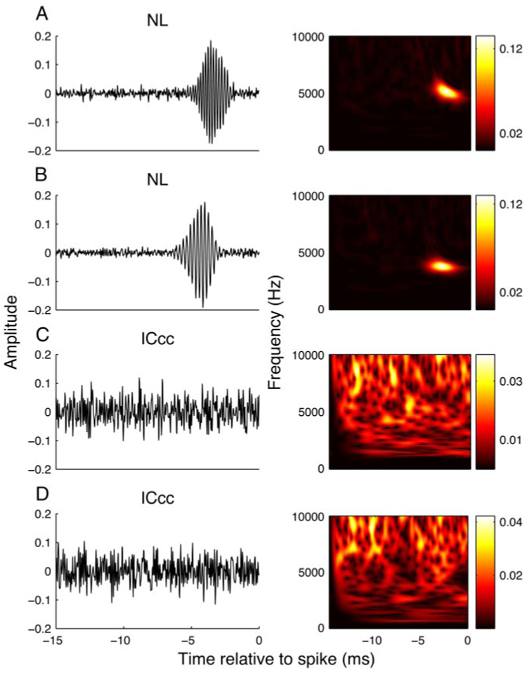
Examples of spike-triggered averages. Shown are examples of the spike-triggered averages of nucleus laminaris (NL; A, B, left column) and central nucleus of the inferior colliculus (ICcc; C, D, left column) neurons, along with their spectrograms (right column). Abscissa gives the time preceding the spike; color bars are provided for reference, but in the following figures will be omitted. A: 4,135 spikes; B: 4,983 spikes; C: 4,739 spikes; D: 4,835 spikes.

Variability

Phase locking in NL throughout the hearing range of the barn owl would predict that the timing of spikes would convey information about the fine structure of the signal. Consistent with this, when the same noise stimulus is repeatedly presented to an NL neuron, a clear pattern emerges in a raster plot of spike times (Fig. 2A). A similar patterned response is also visible in ICcc neurons (Fig. 2B), despite the lack of phase locking described earlier. To quantify the reproducibility of the response, we used the shuffled autocorrelogram (SAC) method (Joris 2003; Louage et al. 2004). The height of the SAC gives the likelihood that given a spike at time t in one presentation of a stimulus that another presentation of the same stimulus will elicit a spike at the same time; the width of the peak of the SAC gives a measure of how much jitter in spike timing is present (Fig. 2, C and D). We note that the SACs of ICcc neurons are in general smooth, indicating a relatively normal distribution of jitter (Fig. 2D). In contrast, NL neurons tended to demonstrate peaks (Fig. 1C), suggesting that jitter in NL neurons tends to occur preferentially at multiples of the period of the preferred frequency of that neuron.

FIG. 2.

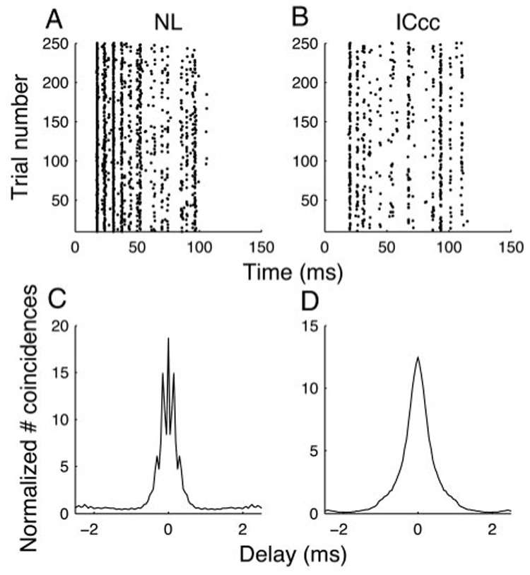
Patterned response in NL and ICcc. Example spike rasters for an NL (A) and an ICcc (B) neuron, using repeated presentation of identical broadband stimuli. C and D: respective shuffled autocorrelograms (SACs) for A and B. Note the fine timescale modulation of the NL SAC, which arises as a result of the phase locking of the neuron, is absent in the ICcc SAC. Despite that, their outer half-height widths are similar.

Both NL and ICcc showed a low amount of jitter, as measured by the SAC half-height width (Fig. 3A). The two populations were not significantly different (NL: Q₁ = 0.44 ms, Q₂ = 0.74 ms, Q₃ = 1.06 ms; ICcc: Q₁ = 0.60 ms, Q₂ = 0.83 ms, Q₃ = 1.03 ms; medians not different by Kruskal–Wallis, P > 0.2). The SAC heights also indicated a high probability of spikes reoccurring at fixed times and there was no significant difference in this regard between the two nuclei (Fig. 3B; NL: Q₁ = 2.60 ms, Q₂ = 3.63 ms, Q₃ = 3.89 ms; ICcc: Q₁ = 2.59 ms, Q₂ = 3.32 ms, Q₃ = 5.08 ms; medians not different by Kruskal–Wallis, P > 0.5). Thus both NL and ICcc display jitter on the submillisecond scale, indicating that this level of temporal precision is maintained through the ascending pathway.

FIG. 3.

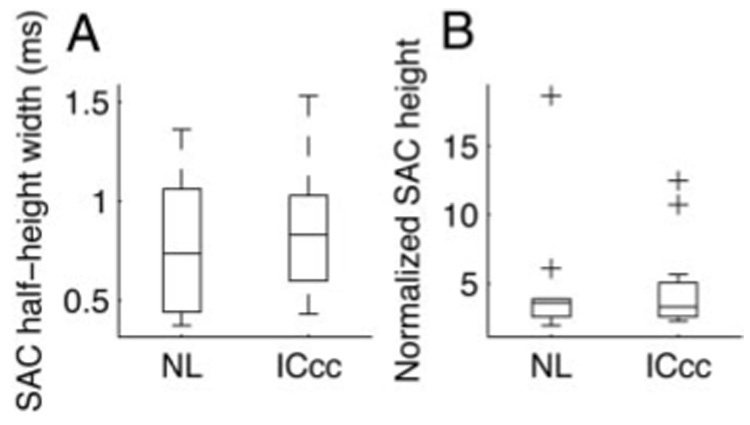
Variability in NL and ICcc. A: half-height widths of the SACs for NL and ICcc neurons. B: maximum height of the SACs for NL and ICcc neurons. Boxes extend from lower quartile to upper quartile of the sample, with the center line marking the median. Outliers (+) are data points >1.5-fold the interquartile range of the sample.

Spectral tuning

As described earlier, the STA requires synchrony to the phase of the stimulus. However, there is ample evidence that the higher auditory centers of both mammals (Batra et al. 1989; Joris 2003; Yin et al. 1984) and owls (Keller and Takahashi 2000) can lock to the power transients of particular frequency bands within the stimulus regardless of phase. This synchrony can be thought of as a locking to the amplitude envelope imposed on the signal by the effective band-pass of the neuron and is thus referred to as envelope coding. To explore this possibility, we also considered the spectrotemporal receptive field (STRF) (see METHODS), which gives the power in each frequency channel as a function of time, independent from the phase of the stimulus. In all neurons recorded in both NL and in ICcc, STRFs were present, which is consistent with envelope coding being present in the neurons of both nuclei (Fig. 4). The shapes of the STRFs were qualitatively similar in all cases and for both nuclei. In all neurons examined, the STRF had an excitatory peak at a latency range predicted by previous physiological data, followed by an inhibitory trough. Because we saw no evidence for an inhibitory mechanism in the spike-triggered average for NL neurons, the trough most likely arises from refractory period effects (Eggermont et al. 1983b). In other words, because we expect the neuron is likely to spike near the onset of an occurrence of a spike-triggering feature; this leads statistically to a greater likelihood that a spike-triggering feature is preceded by an absence of spike-triggering features. The strength of this likelihood is dependent on the refractory period, with shorter refractory periods causing a less-prominent effect.

FIG. 4.

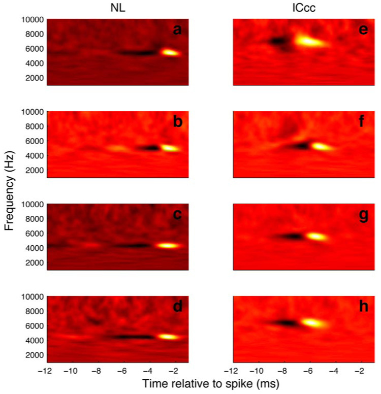
Examples of STRFs estimated for 4 NL (A–D) and ICcc (E–H) units.

Consistent with previous reports based on isointensity frequency-tuning curves (Christianson and Peña 2006) we observed a dependency of bandwidth on center frequency in both nuclei (Fig. 5) in the STRF (NL regression: 0.10x + 224 Hz, P < 0.01; IC regression: 0.11x + 107 Hz, P < 10⁻⁶). These regressions were not significantly different (F-test, P > 0.9), indicating that the spectral tuning ranges seen in ICcc are unchanged from those in NL.

FIG. 5.

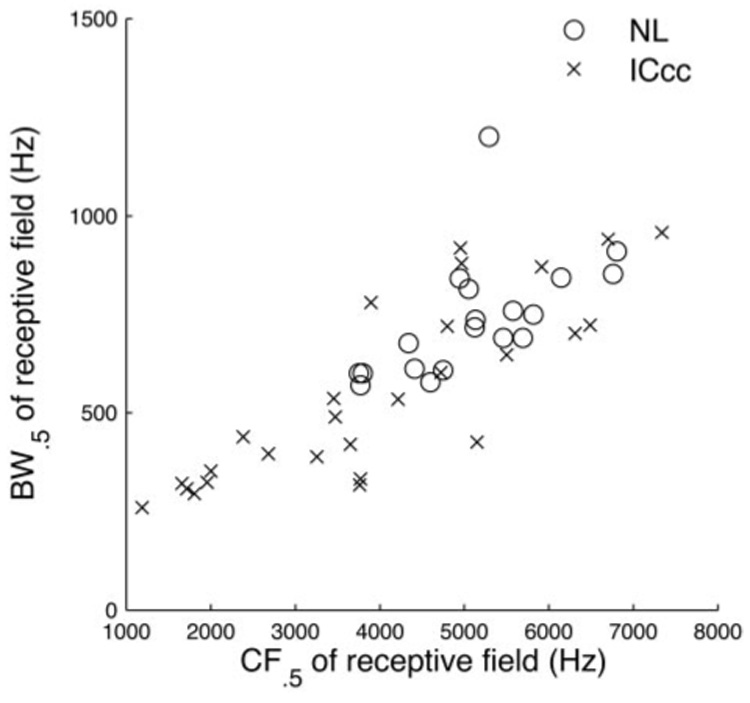
Bandwidths (BWs) of the receptive fields. BW_0.5 of the spectrotemporal receptive fields (STRFs) of NL neurons (circles) and ICcc neurons (crosses) plotted against the 0.5 centered frequency (CF_0.5). There is no evidence for a difference in distribution between the 2 populations (P < 0.9).

Temporal tuning

There is reason to believe that neurons in NL possess very short membrane time constants and thus relatively short temporal integration windows (Gertsner et al. 1996). Thus it might be that ICcc neurons have STRFs that are extended in temporal extent arising from averaging over greater time periods to effect the reduction of noise in ITD encoding (Christianson and Peña 2006); if this were the case, it would be expected that the values of the stimulus over a greater period of time could influence response and thus that the TW_0.5 would be larger in ICcc neurons. In ICcc, there was no correlation between CF_0.5 and TW_0.5 (Fig. 6A; P > 0.4). A weak correlation was present in NL (P < 0.01), but this is likely the result of a small sample size at higher frequencies; removing the two neurons with CF_0.5 >6,500 Hz removed the correlation (P > 0.05). Pooling the observed TW_0.5 across frequency, there was no statistically significant difference between the neurons of the two nuclei (P > 0.7). These results are based on a definition of TW_0.5 that neglected the following inhibitory trough (that is, it considers only the temporal extent of the excitatory peak), but including the trough did not affect the conclusions presented here. Thus there is no evidence that ICcc neurons integrate their responses over a longer period of time than NL neurons and thus that noise reduction for ITD tuning is mainly the result of a mechanism that pools across inputs rather than one that pools across time.

FIG. 6.

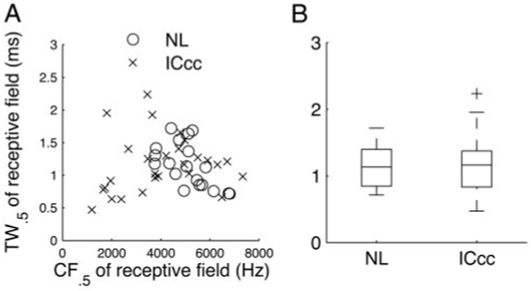
Temporal widths (TWs) of the receptive fields. A: TW_0.5 of the STRFs of NL (circles) and ICcc neurons (crosses) plotted against the CF_0.5. There was no apparent correlation between the parameters for ICcc and a weak and possibly artifactual correlation for NL (see text). B: boxplot of the distribution of temporal widths seen in the two nuclei. Median TW_0.5 was not significantly different (P > 0.7).

Separability of the STRFs

Although NL and ICcc STRFs have similar spectral and temporal extent, it may be that there is some difference in shape that reflects a change in spectral processing from NL and ICcc. One way to quantify this is the degree of separability of the STRFs: that is, can the STRF be considered the product of individual time and frequency tuning functions? Alternatively, there may be nontrivial time–frequency interactions in the receptive field, which could be consistent with a tuning to frequency-modulated tone sweeps, for instance. Taking the SVD of the STRF and then observing the fractional energy of the singular value components can address this question. For a separable STRF, the fractional energy of the first singular value will dominate over that of the other values. When we perform this analysis on our data set (Fig. 6), we see that for both nuclei the fractional energy of the first component dominates (fractional energy of the first singular value for NL: 77 ± 8%; for ICcc: 65 ± 17%), whereas the others lay along a characteristic exponential line, which suggests that the spectral and temporal components of the STRFs are relatively separable: that is, that the STRF can be well approximated as the product of a spectral and a temporal tuning vector, although as Fig. 7 illustrates there was a trend toward a small downward sweep in the STRFs. There is also no strong evidence that either nucleus is more separable than the other (P > 0.01), which argues against any dramatic changes in the shape of the STRFs. The fact that the fractional energies are different at the P < 0.05 level leaves open the possibility that there is some subtle change in the STRF shape between the two nuclei, perhaps reflecting the beginning of stimulus-specific spectrotemporal tuning.

FIG. 7.

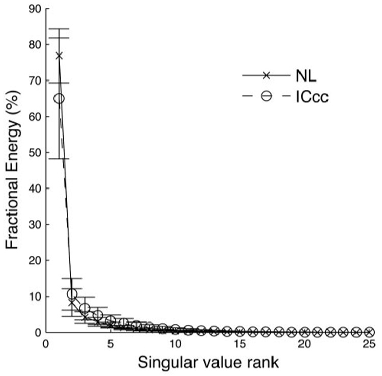
Mean fractional energy of the singular value decomposition (SVD) of the STRFs for all NL (×) and ICcc (○) neurons. Mean fractional energy of the first singular value for NL neurons: 77 ± 8%. Mean fractional energy of the first singular value for ICcc neurons: 65 ± 17%.

Prediction of response

In principle, descriptions of the receptive fields of a neuron should be able to predict the neuron’s response to novel stimuli (Eggermont et al. 1983a; Linden et al. 2003; Theunissen et al. 2000). The degree to which the prediction matches the true neuronal response then provides a measure of the sufficiency of the model: in this case, to what degree the STRF is a complete description of the behavior of the neuron. Because the STRF is a linear model, if some nonlinear processing of spectral cues was introduced from NL to ICcc, it would not be evident in the preceding analysis, but we would expect that the ability of the STRF to predict responses in ICcc to be degraded compared with the performance in NL.

We were able to test this in the neurons for which we collected frozen noise data. In NL, it was possible to get a good prediction of the firing rate in response to a novel stimulus (because the frozen noise data were not included in the computation of the PESE), as seen in Fig. 8A. In our data set, a linear model was able to account for 39 ± 12% of the variance of NL neurons (Fig. 8B); this is comparable to the predictive ability of STRFs in ICls (Keller and Takahashi 2000), auditory cortex (Linden et al. 2003), and in the auditory midbrain of the grass frog (Eggermont et al. 1983a). ICcc neurons were also well estimated by the STRF (Fig. 8C) and the performance across the ICcc population (31 ± 12% of variance explained) was not significantly different from the performance in NL (ANOVA, P > 0.1). Thus although we cannot rule out the possibility that there is some nonlinear difference in spectrotemporal encoding between NL and ICcc neurons, our data do not suggest such a conclusion.

FIG. 8.

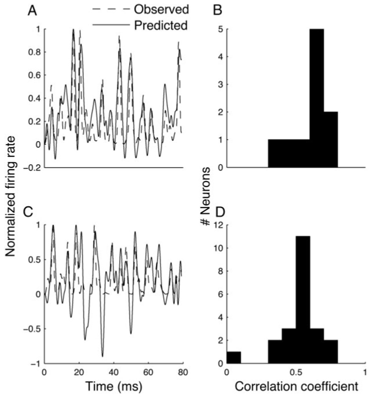
Prediction of response. A: poststimulus time histogram (PSTH) of NL neuron (dashed line) in response to frozen noise, overlaid with the prediction of response based on the STRF (solid line). Because our model is linear, and therefore does not include the effects of rectification, the model predicts negative firing rates, leading to the visible troughs not present in the PSTH. This trend is expected to be more conspicuous in ICcc, where strong rectification effects have been demonstrated (Christianson and Peña 2006). B: distribution of correlation coefficients between predicted and observed firing rates (>80 ms of stimulus) for 10 NL neurons. C and D are similarly for 22 ICcc neurons.

Envelope coding of ITD

Neurons in the cat IC were also previously identified that appear to synchronize to the cochlea-induced envelope pattern (Chase and Young 2006; Joris 2003). However, synchronization to amplitude modulations, both of the sound’s intrinsic waveform (Joris and Yin 1992, 1998) and of the cochlear output waveform (Louage et al. 2004), was described in lower auditory centers, leaving open the possibility that phase-locking and envelope-locking neurons represent two distinct populations throughout the ascending auditory pathway. Although we did not observe any NL neurons that did not phase lock, we would like to rule out the possibility that the ICcc neurons were driven by a subset of purely envelope-locking NL neurons.

A simple test for this comes from polarity tolerance. Normally, the rate-ITD function obtained with anticorrelated broadband noise presented to the two ears is the inverse of the rate-ITD function obtained with perfectly correlated noise (Yin et al. 1987). However, some rate-ITD functions do not invert under anticorrelated stimulation (Joris 2003). Because the amplitude envelope of a signal is invariant with respect to inversion (Hartmann 1997), the absence of inversion with anticorrelated noise is consistent with a computation of ITD based on the cross-correlation of signals synchronized to the envelope. Therefore we collected rate-ITD functions in both correlated and anticorrelated cases for 17 ICcc neurons. In all cases, we observed a significant negative correlation between the two rate-ITD functions (P < 10⁻⁴), indicating that the inputs to these neurons had been locked to ongoing phase, and not the envelope, when computing the ITD.

DISCUSSION

NL neurons project to ICcc (Takahashi and Konishi 1988). Our results show, for the first time, that phase locking to frequencies >1 kHz in the barn owl is significantly reduced in a single step. Work in mammalian systems demonstrated a decline in the ability of neurons to phase lock through ascending auditory stations, although phase locking can still be observed as high as auditory cortex (Liu et al. 2006; Wallace et al. 2002; Winter and Palmer 1990). Our results indicate that it is possible for ascending auditory centers to maintain comparable spectrotemporal tuning, in the sense of having STRFs with equal frequency and temporal tuning parameters, while discarding the phase information used by their inputs. Although a representation of phase is necessary for the computation of ITD, the many documented specializations of the early ITD pathway (Carr 1993; Trussel 1999) suggest that it is costly to preserve. Thus in terms of the representation of the dynamic spectral properties of the signal, it may be more efficient to maintain precision on the millisecond scale while allowing jitter to accumulate at a submillisecond scale, which would then result in a decline in phase-locking quality.

Previous studies in the barn owl (Keller and Takahashi 2000), as well as amphibian (Hermes et al. 1981) and mammalian models (Carney and Yin 1989), demonstrated patterned (that is, stimulus-locked) responses in the midbrain using broadband noise. However, because of the segregation of sound localization cues in the barn owl, it is not immediately clear whether these responses emerge from the ITD pathway or the ILD pathway. Taken all together, our results suggest that the population activity of the nuclei of the ITD pathway, and specifically ICcc, can be treated as a dynamic spectrum analyzer with a temporal resolution of approximately a millisecond. Although this does not rule out any role of the ILD-sensitive neurons in the generation of spectral tuning in higher auditory centers, it does argue against the possibility that the spectrotemporal tuning in ICls neurons reported by Keller and Takahashi (2000) is attributed solely to the inputs from the ILD-sensitive neurons.

We did not examine the effect on the STRF of varying ITD because the rectification and large dynamic range of the rate-ITD functions of ICcc neurons (Christianson and Peña 2006) made collecting a sufficient number of spikes for nonpeak ITDs prohibitive. However, raster plots from the work of Carney and Yin (1989) indicate that the timing of spikes, if not their number, is relatively invariant to changes in the ITD in the cat IC; this is confirmed by the work demonstrating that spike timing does not appear to convey information related to the ITD (Chase and Young 2006). Previous work in owls (Keller and Takahashi 2000) demonstrated that STRFs of neurons in the ICls, to which ICcc projects, are also invariant under changes in ITD. Thus any dependency on ITD of STRFs for NL and ICcc neurons is likely to be explainable by a modulation in gain resulting from the dependency of mean firing rate on ITD.

In previous work, we showed that the transition from NL to ICcc acts as a noise-elimination phase in the representation of ITD (Christianson and Peña 2006). It might be expected that this improvement in the encoding of a spatial location cue might come at the expense of the representation of the spectral content; this is especially true in the barn owl, where it is established that there is a frequency convergence to resolve ITD coding ambiguity (Mazer 1998; Saberi et al. 1999; Takahashi and Konishi 1986). Here, we demonstrate that this is not the case. The conclusion is thus that the pooling that produces the reduction in ITD encoding noise must occur over a population of NL neurons with extremely similar spectrotemporal tuning. This may not be as difficult to arrange as it may appear. Theoretical work suggests that the neurons that compute the ITD should behave as cross-correlators (Licklider 1959), which experimental work supports (Yin and Chan 1990). One of the properties of cross-correlation is that the shape of the cross-correlation function (in this case, the rate-ITD function) should be determined by the spectral tuning of the cross-correlator, known as the Wiener–Khinchin relationship. Although the experimental evidence in support of this property is weak (Yin and Chan 1990), it suggests that with an assumption of a moderate degree of homogeneity in the properties of NL neurons, the expectation would be that similar spectral tuning should accompany similar ITD tuning.

At first glance, the observation from Christianson and Peña (2006) that NL neurons are noisy compared with ICcc neurons would seem to be in conflict with our observation that the variability in response to frozen noise stimulation was the same in both nuclei. In fact, the noise in the NL rate-ITD functions is likely to be the result of the spectrotemporal tuning itself. Because white noise has a uniform spectrum only when averaged over time, we would expect the firing rate over small time windows to be influenced to a large degree by the instantaneous power spectrum of the signal. The result that the STRFs and the SACs of both NL and ICcc neurons are similar suggests that the variability in response arising from spectral properties of the signal is the same in both nuclei, and we have observed that the overall variability in firing rate as a function of mean firing rate was similar in both NL and ICcc (Christianson and Peña 2006). Thus it is likely that a primary source of “noise” in the rate-ITD function is a result of the variations in spike timing linked to spectrotemporal attributes of the sound, which is consistent with work done in cats indicating that ITD information is not carried by precise spike timing (Chase and Young 2006). However, in ICcc the increase in overall dynamic range in the rate-ITD function (Christianson and Peña 2006) allows that the variation in mean firing rate resulting from the firing patterns related to the spectral properties of different signals with the same ITD be small compared with the variation in mean firing rate resulting from changes in the ITD. As such, this constitutes an elegant implementation of simultaneous rate- and timing-based coding strategies to represent multiple stimulus parameters within the limited language of neuronal spiking.

REFERENCES

- Arthur BJ. Sensitivity to spectral interaural intensity difference cues in space-specific neurons of the barn owl. J Comp Physiol A Sens Neural Behav Physiol. 2004;190:91–104. doi: 10.1007/s00359-003-0476-1. [DOI] [PubMed] [Google Scholar]
- Batra R, Kuwada S, Stanford TR. Temporal coding of envelopes and their interaural delays in the inferior colliculus of the unanesthetized rabbit. J Neurophysiol. 1989;61:257–268. doi: 10.1152/jn.1989.61.2.257. [DOI] [PubMed] [Google Scholar]
- Brenowitz EA. The contribution of temporal song cues to species recognition in the red-winged blackbird. Anim Behav. 1983;31:1116–1127. [Google Scholar]
- Carney LH, Yin TC. Response of low-frequency cells in the inferior colliculus to interaural time differences of clicks: excitatory and inhibitory components. J Neurophysiol. 1989;62:144–161. doi: 10.1152/jn.1989.62.1.144. [DOI] [PubMed] [Google Scholar]
- Carr CE. Delay line models of sound localization in the barn owl. Am Zool. 1993;33:79–85. [Google Scholar]
- Carr CE, Konishi M. A circuit for detection of interaural time differences in the brain stem of the barn owl. J Neurosci. 1990;10:3277–3246. doi: 10.1523/JNEUROSCI.10-10-03227.1990. [DOI] [PMC free article] [PubMed] [Google Scholar]
- Chase SM, Young ED. Spike-timing codes enhance the representation of simultaneous sound-localization cues in the inferior colliculus. J Neurosci. 2006;26:3889–3898. doi: 10.1523/JNEUROSCI.4986-05.2006. [DOI] [PMC free article] [PubMed] [Google Scholar]
- Christianson GB, Peña JL. Noise reduction of coincidence detector outputs by the inferior colliculus of the barn owl. J Neurosci. 2006;26:5948–5954. doi: 10.1523/JNEUROSCI.0220-06.2006. [DOI] [PMC free article] [PubMed] [Google Scholar]
- de Boer E, de Jongh HR. On cochlear encoding: potentialities and limitations of the reverse-correlation technique. J Acoust Soc Am. 1978;63:115–135. doi: 10.1121/1.381704. [DOI] [PubMed] [Google Scholar]
- Depireux DA, Simon JZ, Klein DJ, Shamma SA. Spectro-temporal response field characterizations with dynamic ripples in ferret primary auditory cortex. J Neurophysiol. 2001;85:1220–1234. doi: 10.1152/jn.2001.85.3.1220. [DOI] [PubMed] [Google Scholar]
- Drullman R, Festen HM, Plomp R. Effect of temporal envelope smearing on speech recognition. J Acoust Soc Am. 1994;95:1053–1064. doi: 10.1121/1.408467. [DOI] [PubMed] [Google Scholar]
- Eggermont J. Wiener and Volterra analyses applied to the auditory system. Hear Res. 1993;10:191–202. doi: 10.1016/0378-5955(93)90139-r. [DOI] [PubMed] [Google Scholar]
- Eggermont JJ, Aertsen AM, Johannesma PI. Prediction of the responses of auditory neurons in the midbrain of the grass frog based on the spectrotemporal receptive field. Hear Res. 1983a;10:191–202. doi: 10.1016/0378-5955(83)90053-9. [DOI] [PubMed] [Google Scholar]
- Eggermont JJ, Johannesma PIM, Aertsen AMHJ. Reverse-correlation methods in auditory research. Q Rev Biophys. 1983b;16:341–414. doi: 10.1017/s0033583500005126. [DOI] [PubMed] [Google Scholar]
- Gertsner W, Kempter R, van Hemmen JL, Wagner H. A neuronal learning rule for sub-millisecond temporal coding. Nature. 1996;383:76–78. doi: 10.1038/383076a0. [DOI] [PubMed] [Google Scholar]
- Grantham DW, Wightman FL. Detectability of varying interaural temporal differences. J Acoust Soc Am. 1978;63:511–523. doi: 10.1121/1.381751. [DOI] [PubMed] [Google Scholar]
- Hartmann WM. Signals, Sound, and Sensation. New York: Springer-Verlag; 1997. p. 416. [Google Scholar]
- Hermes DJ, Aertsen AM, Johannesma PIM, Eggermont JJ. Spectrotemporal characteristics of single units in the auditory midbrain of the lightly anaesthetized grass frog (Rana temporaria L) investigated with noise stimuli. Hear Res. 1981;5:147–178. doi: 10.1016/0378-5955(81)90043-5. [DOI] [PubMed] [Google Scholar]
- Joris PX. Interaural time sensitivity dominated by cochlea-induced envelope patterns. J Neurosci. 2003;23:6345–6350. doi: 10.1523/JNEUROSCI.23-15-06345.2003. [DOI] [PMC free article] [PubMed] [Google Scholar]
- Joris PX, Yin TCT. Responses to amplitude-modulated tones in the auditory nerve of the cat. J Acoust Soc Am. 1992;91:215–232. doi: 10.1121/1.402757. [DOI] [PubMed] [Google Scholar]
- Joris PX, Yin TCT. Envelope coding in the lateral superior olive. III. Comparison with afferent pathways. J Neurophysiol. 1998;73:253–269. doi: 10.1152/jn.1998.79.1.253. [DOI] [PubMed] [Google Scholar]
- Keller CH, Takahashi TT. Representation of temporal features of complex sounds by the discharge patterns of neurons in the owl’s inferior colliculus. J Neurophysiol. 2000;84:2638–2650. doi: 10.1152/jn.2000.84.5.2638. [DOI] [PubMed] [Google Scholar]
- Kim PJ, Young ED. Comparative analysis of spectro-temporal receptive fields, reverse correlation functions, and frequency tuning curves of auditory-nerve fibers. J Acoust Soc Am. 1994;95:410–422. doi: 10.1121/1.408335. [DOI] [PubMed] [Google Scholar]
- Klein DJ, Depireux DA, Simon JZ, Shamma SA. Robust spectrotemporal reverse correlation for the auditory system: optimizing stimulus design. J Comput Neurosci. 2000;9:85–111. doi: 10.1023/a:1008990412183. [DOI] [PubMed] [Google Scholar]
- Konishi M. How the owl tracks its prey. Am Scientist. 1973;61:414–424. [Google Scholar]
- Konishi M, Kenuk AS. Discrimination of noise spectra by memory in the barn owl. J Comp Physiol. 1975;97:55–58. [Google Scholar]
- Köppl C. Phase locking to high frequencies in the auditory nerve and cochlear nucleus magnocellularis of the barn owl, Tyto alba. J Neurosci. 1997;17:3312–3321. doi: 10.1523/JNEUROSCI.17-09-03312.1997. [DOI] [PMC free article] [PubMed] [Google Scholar]
- Lewis ER, Henry KR, Yamada WM. Tuning and timing of excitation and inhibition in primary auditory nerve fibers. Hear Res. 2002;171:13–31. doi: 10.1016/s0378-5955(02)00290-3. [DOI] [PubMed] [Google Scholar]
- Licklider JCR. Three auditory theories. In: Koch S, editor. Psychology: A Study of a Science. New York: McGraw-Hill; 1959. [Google Scholar]
- Linden JF, Liu RC, Sahani M, Schreiner CE, Merzenich MM. Spectrotemporal structure of receptive fields in areas AI and AAF of mouse auditory cortex. J Neurophysiol. 2003;90:2660–2675. doi: 10.1152/jn.00751.2002. [DOI] [PubMed] [Google Scholar]
- Liu L, Palmer AR, Wallace MN. Phase-locked responses to pure tones in the inferior colliculus. J Neurophysiol. 2006;95:1926–1935. doi: 10.1152/jn.00497.2005. [DOI] [PubMed] [Google Scholar]
- Louage DHG, van der Heijden M, Joris PX. Temporal properties of responses to broadband noise in the auditory nerve. J Neurophysiol. 2004;91:2051–2065. doi: 10.1152/jn.00816.2003. [DOI] [PubMed] [Google Scholar]
- Mazer J. How the owl resolves auditory coding ambiguity. Proc Natl Acad Sci USA. 1998;95:10932–10937. doi: 10.1073/pnas.95.18.10932. [DOI] [PMC free article] [PubMed] [Google Scholar]
- Peña JL, Viete S, Albeck Y, Konishi M. Tolerance to sound intensity of binaural coincidence detection in the nucleus laminaris of the owl. J Neurosci. 1996;16:7046–7054. doi: 10.1523/JNEUROSCI.16-21-07046.1996. [DOI] [PMC free article] [PubMed] [Google Scholar]
- Peña JL, Viete S, Funabiki K, Saberi K, Konishi M. Cochlear and neural delays for coincidence detection in owls. J Neurosci. 2001;21:9455–9459. doi: 10.1523/JNEUROSCI.21-23-09455.2001. [DOI] [PMC free article] [PubMed] [Google Scholar]
- Quine DB, Konishi M. Absolute frequency discrimination in the barn owl. J Comp Physiol. 1974;93:347–360. [Google Scholar]
- Ross S. A First Course in Probability. 4th ed. New York: Macmillan College Publishing; 1994. [Google Scholar]
- Rust NC, Schwartz O, Movshon JA, Simoncelli E. Spike-triggered characterizations of excitatory and suppressive stimulus dimensions in monkey V1. Neurocomputing. 2004;58– 60:793–799. [Google Scholar]
- Saberi K, Takahashi Y, Farahbod H, Konishi M. Neural basis of an auditory illusion and its elimination in owls. Nat Neurosci. 1999;2:656–659. doi: 10.1038/10212. [DOI] [PubMed] [Google Scholar]
- Shannon RV, Zeng FG, Kamath V, Wygonski J, Ekelid M. Speech recognition with primarily temporal cues. Science. 1995;270:303–304. doi: 10.1126/science.270.5234.303. [DOI] [PubMed] [Google Scholar]
- Sullivan WE, Konishi M. Segregation of stimulus phase and intensity coding in the cochlear nucleus of the barn owl. J Neurosci. 1984;4:1787–1799. doi: 10.1523/JNEUROSCI.04-07-01787.1984. [DOI] [PMC free article] [PubMed] [Google Scholar]
- Takahashi TT, Konishi M. Selectivity for interaural time difference in the owl’s midbrain. J Neurosci. 1986;6:3413–3422. doi: 10.1523/JNEUROSCI.06-12-03413.1986. [DOI] [PMC free article] [PubMed] [Google Scholar]
- Takahashi TT, Konishi M. Projections of the cochlear nuclei and nucleus laminaris to the inferior colliculus of the barn owl. J Comp Neurol. 1988;274:190–211. doi: 10.1002/cne.902740206. [DOI] [PubMed] [Google Scholar]
- Takahashi TT, Wagner H, Konishi M. Role of commissural projections in the representation of bilateral auditory space in the barn owl’s inferior colliculus. J Comp Neurol. 1989;281:545–554. doi: 10.1002/cne.902810405. [DOI] [PubMed] [Google Scholar]
- Theunissen FE, Sen K, Doupe AJ. Spectral-temporal receptive fields of nonlinear auditory neurons obtained using natural sounds. J Neurosci. 2000;20:2315–2331. doi: 10.1523/JNEUROSCI.20-06-02315.2000. [DOI] [PMC free article] [PubMed] [Google Scholar]
- Trussell LO. Synaptic mechanisms for coding timing in auditory neurons. Annu Rev Physiol. 1999;61:477–496. doi: 10.1146/annurev.physiol.61.1.477. [DOI] [PubMed] [Google Scholar]
- Wallace MN, Shackleton TM, Palmer AR. Phase-locked responses to pure tones in the primary auditory cortex. Hear Res. 2002;172:160–171. doi: 10.1016/s0378-5955(02)00580-4. [DOI] [PubMed] [Google Scholar]
- Winter IM, Palmer AR. Responses of single units in the anteroventral cochlear nucleus of the guinea pig. Hear Res. 1990;44:161–178. doi: 10.1016/0378-5955(90)90078-4. [DOI] [PubMed] [Google Scholar]
- Wright BA, Lombardino LJ, King WM, Puranik CS, Leonard CM, Merzenich MM. Deficits in auditory temporal and spectral resolution in language-impaired children. Nature. 1997;387:176–178. doi: 10.1038/387176a0. [DOI] [PubMed] [Google Scholar]
- Yamada WM, Lewis ER. Predicting the temporal responses of non-phase-locking bullfrog auditory units to complex auditory waveforms. Hear Res. 1999;130:155–170. doi: 10.1016/s0378-5955(99)00005-2. [DOI] [PubMed] [Google Scholar]
- Yin TCT, Chan JCK. Interaural time sensitivity in the medial superior olive of the cat. J Neurophysiol. 1990;64:465–488. doi: 10.1152/jn.1990.64.2.465. [DOI] [PubMed] [Google Scholar]
- Yin TCT, Chan JCK, Carney LH. Effects of interaural time delays of noise stimuli on low-frequency cells in the cat’s inferior colliculus. III. Evidence for cross-correlation. J Neurophysiol. 1987;58:562–583. doi: 10.1152/jn.1987.58.3.562. [DOI] [PubMed] [Google Scholar]
- Yin TCT, Kuwada S, Sujaku Y. Interaural time sensitivity of high-frequency neurons in the inferior colliculus. J Acoust Soc Am. 1984;76:1401–1410. doi: 10.1121/1.391457. [DOI] [PubMed] [Google Scholar]
- Zhang XD, Heinz MG, Bruce IC, Carney LH. A phenomenological model for the responses of auditory-nerve fibers: I. Nonlinear tuning with compression and suppression. J Acoust Soc Am. 2001;109:648–670. doi: 10.1121/1.1336503. [DOI] [PubMed] [Google Scholar]