Fast and Accurate Method for Determining Molar Concentrations of Metabolites in Complex Solutions from Two-Dimensional ¹H-¹³C NMR Spectra

Abstract

One-dimensional (1D) ¹H nuclear magnetic resonance (NMR) spectroscopy is used extensively for high-throughput analysis of metabolites in biological fluids and tissue extracts. Typically, such spectra are treated as multivariate statistical objects rather than as collections of quantifiable metabolites. We report here a two-dimensional (2D) ¹H-¹³C NMR strategy (Fast Metabolite Quantification, FMQ by NMR) for identifying and quantifying the ∼40 most abundant metabolites in biological samples. To validate this technique, we prepared mixtures of synthetic compounds and extracts from Arabidopsis thaliana, Saccharomyces cerevisiae and Medicago sativa. We show that accurate (technical error 2.7%) molar concentrations can be determined in 12 minutes using our quantitative 2D ¹H-¹³C NMR strategy. In contrast, traditional 1D ¹H NMR analysis resulted in 16.2% technical error under nearly ideal conditions. We propose FMQ by NMR as a practical alternative to 1D ¹H NMR for metabolomics studies in which 200-400 mg (preextraction dry weight) samples can be obtained.

One-dimensional (1D) ¹H NMR spectroscopy has been used for decades as an analytical tool for identifying small molecules and measuring their concentrations.^{1, 2} Traditionally, quantitative analysis by NMR has been restricted to relatively simple mixtures with minimal peak overlap. In these applications, 1D ¹H NMR is a natural choice, because its peaks scale linearly with concentration and its analytical precision is usually independent of the chemical properties of target molecules. Recently, interest has surged in using NMR for high-throughput analysis of complex biological processes at the metabolic level.^{3, 4} These studies, defined as “metabolomics” or “metabonomics”, place an emphasis on biomarker discovery or disease classification and are typically centered on unfractionated biological fluids and tissue extracts. 1D ¹H NMR spectra of these samples typically contain hundreds of overlapping resonances (Figure 1) that make traditional NMR-based analytical practices, such as resonance assignment and accurate peak integration, a challenging prospect. As a result, sophisticated statistical tools have been developed to translate spectral data into biologically meaningful information.^{4, 5}

Figure 1.

(a) One-dimensional ¹H NMR spectrum of an equimolar mixture of the 26 small molecule standards listed in Supplementary Table 1. (b) Two-dimensional ¹H-¹³C HSQC NMR spectra of the same synthetic mixture (red) overlaid onto a spectrum of aqueous whole-plant extract from Arabidopsis thaliana (blue).

All statistical tools used for analyzing complex spectra face the same fundamental barrier: overlapped peaks do not scale in the discrete linear fashion that typifies well-isolated peaks. They scale as the sum of the total overlapped resonance. Consequently, multivariate and correlation statistics are reporters of overlapped spectral density, not concentrations of specific compounds. Although peak overlap does not interfere with the reproducibility of traditional analyses,⁶ it does prevent accurate quantification.

Two approaches can be used to overcome this barrier, one mathematical the other experimental. The mathematical approach is to fit overlapped ¹D NMR spectra with modeled peaks. This approach has been successfully applied by Weljie and co-workers.⁷ The experimental approach is to collect NMR spectra that disperse peaks into two or more dimensions. This allows non-overlapped peak intensities to be measured directly.

Two-dimensional NMR (Figure 1) is a well established technique for reducing peak overlap and has been recognized for over ten years as an excellent tool for metabolomics.^8-11 Despite this, published applications of multidimensional NMR in the metabolomics literature have been largely restricted to qualitative analyses. One reason for this is that 2D cross-peak intensities (or volumes) are influenced by a greater number of variables (e.g. uneven excitation, non-uniform relaxation, evolution times, mixing times, etc.) than are 1D ¹H NMR peaks. This non-uniform behavior makes it difficult to translate peak intensities into metabolite concentrations. A second reason is that 2D NMR spectra usually require more time to collect than 1D ¹H spectra. Long NMR acquisition times are impractical for metabolomics studies requiring the analysis of hundreds of samples.

In this paper we introduce a simple experimental protocol, Fast Metabolite Quantification (FMQ) by NMR (Figure 2), for measuring molar concentrations of metabolites in complex solutions using 2D ¹H-¹³C NMR. This method is accurate and allows 2D experiments to be collected in as little as 12 minutes. Our method requires that all target metabolites be identified and that 2D ¹H-¹³C NMR spectra of standards have been collected under comparable conditions. Metabolite identification has recently become feasible with three new public databases: the metabolomics extension of the Biological Magnetic Resonance Data Bank (BMRB, www.bmrb.wisc.edu);^{12, 13} the Madison Metabolomics Consortium Database (MMCD, http://mmcd.nmrfam.wisc.edu),¹³ Qiu Cui, I.A.L., Adrian D. Hegeman, Mark E. Anderson, Jing Li, Christopher F. Schulte, W.M.W, Hamid R. Eghbalnia, M.R.S, and J.L.M., manuscript in preparation; and the Human Metabolome Project (HMP, www.metabolomics.ca).¹⁴ We describe how to identify metabolites using these tools and demonstrate the process by identifying and quantifying metabolites in Arabidopsis thaliana, Saccharomyces cerevisiae and Medicago sativa tissue extracts. In addition, we estimate the technical error associated with 1D and 2D NMR analyses of complex mixtures. The protocol we describe is a general quantitative procedure that can be applied to any biological system in which 200-400 mg (mass of dry tissue prior to extraction) samples can be obtained.

Figure 2.

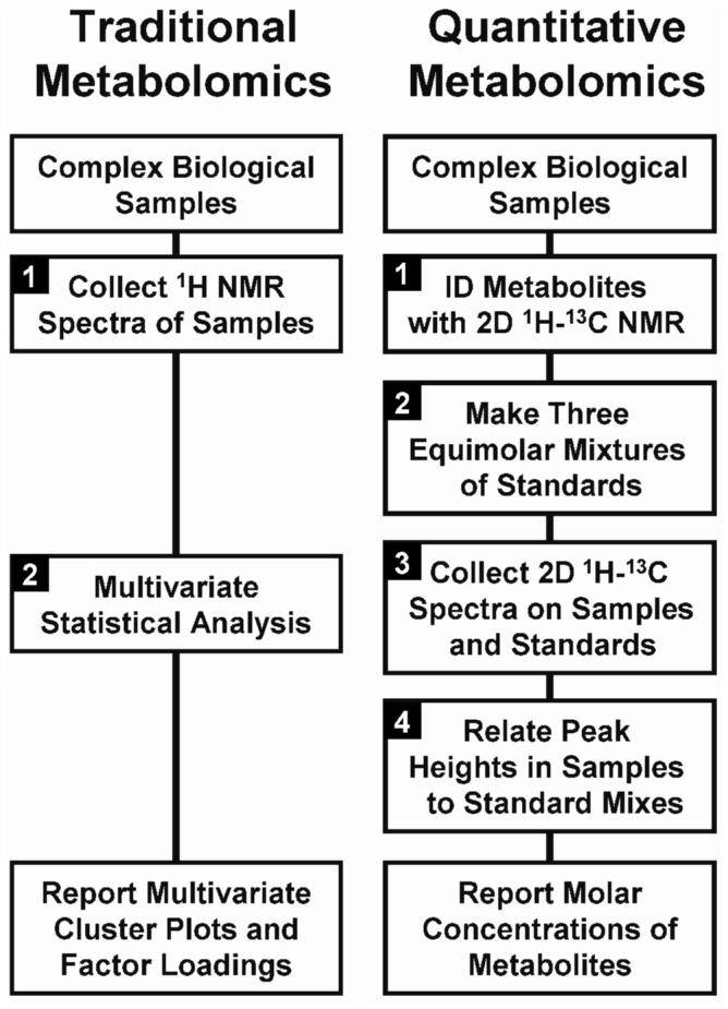
(Left) The two-step experimental design used in traditional metabolomics, which typically reports multivariate statistics related to spectra. (Right) Our four-step quantitative metabolomics protocol, “FMQ by NMR”, which yields molar concentrations for all identified metabolites.

EXPERIMENTAL SECTION

Experimental Rationale

One of the main purposes of this study was to evaluate 1D ¹H NMR and 2D ¹H ¹³C NMR as quantitative tools for metabolic profiling. To do this, we identified ∼80% of the NMR-observable metabolites present in Arabidopsis, Saccharomyces and Medicago extracts. A subset of these compounds was selected to represent an average extract, and several synthetic mixtures of pure compounds were prepared. All of the error estimates reported in this study are based on the synthetic mixtures rather than real biological extracts. This approach allowed us to measure the absolute error associated with the experimental techniques. Although our synthetic samples contained considerably fewer compounds than a real extract, the mixtures were created with biologically realistic concentrations and chemical diversity.

Plant Growth and Tissue Extraction

Arabidopsis thaliana seeds were germinated and grown in sterile liquid cultures of MS medium.¹⁵ Seedlings were incubated under continuous illumination on a shaker platform. After two weeks of growth, plants were harvested, washed in ddH₂O and flash-frozen in liquid nitrogen. Wild type (DS10) Saccharomyces cerevisiae were prepared by growing a culture in YPD medium until cells had reached the stationary phase (optical density of 15). Cells suspensions were centrifuged, and the pellet was washed in 20 volumes of phosphate buffered saline (10 mM sodium phosphate, 150 mM NaCl, pH 7.0). Washed cell suspensions were centrifuged, and the remaining cell pellet was flash frozen in liquid nitrogen. Medicago sativa sprouts were obtained from a local grocery store. Sprouts were washed in ddH₂O and flash frozen in liquid nitrogen.

Frozen Arabidopsis seedlings, Medicago sprouts, and Saccharomyces cells were lyophilized for 48 h and homogenized in a coffee grinder. 400 mg of each dry homogenate was suspended in 16 mL of boiling ddH₂O and incubated at 100°C in a screw-top 22 mL vial for 15 minutes. Extracts were microfiltered through ddH₂O-washed 3 kDa cutoff spin filters, and the filtrate was lyophilized to a dry powder. The lyophilized extract was suspended in NMR buffer B: D₂O, 5 mM HEPES (4-(2-hydroxylethyl)-1-piperazine ethanesulfonic acid), 500 μM NaN₃ and 500 μM DSS (2,2-dimethylsilapentane-5-sulfonic acid) at a volume-to-weight ratio of 8.75 μL buffer B per milligram extract. The resulting solution was titrated with DCl or NaOD as needed to achieve an observed pH of 7.400 (± 0.004).

Preparation of Synthetic Samples

A total of thirty synthetic mixtures were prepared for the error analysis study. Twenty-four of these samples were designated as “test mixtures”, and six samples were designated as “concentration references.” Both the test mixtures and concentration references contained twenty-six small molecules (see Supplementary Table 1). Twenty-five of these standards were metabolites selected from the larger list of molecules identified in the three biological extracts (see Quantitative Protocol, Step 1). HEPES was also included in the synthetic samples as an internal concentration reference. All mixtures were prepared from weighed pure standards (Sigma-Aldrich) suspended in NMR buffer B and were titrated to an observed pH of 7.400 (+/- 0.004). Test mixtures contained nineteen metabolites with invariant concentrations (all 5 mM) and seven metabolites with variable concentrations ranging from 5.5 to 29.1 mM. Although each test mixture had a unique metabolite profile, the samples were designed to group into six classes with biologically relevant concentrations and standard deviations (see Supplementary Table 2). The six concentration reference samples were prepared with equimolar mixtures of the twenty-six metabolites. These samples contained each metabolite at 2 mM (N=2), 5 mM (N=2), or 10 mM (N=2).

A separate set of biological concentration reference standards was prepared for estimating concentrations in the three tissue extracts. Biological reference samples had a total of 52 metabolites split between three groups. The groups were designed to minimize overlap between metabolites signals in 2D ¹H-¹³C NMR spectra. Biological references were prepared in the same manner as described for the synthetic concentration reference samples.

NMR Spectroscopy

All NMR spectroscopy was carried out at the National Magnetic Resonance Facility in Madison. Spectra were collected on a Varian 600 MHz spectrometer equipped with a triple-resonance (¹H, ¹³C, ¹⁵N, ²H lock) cryogenic probe and a sample changer. The probe was tuned, matched, and shimmed by hand for the first sample. All subsequent samples were collected using an automated shimming and data acquisition macro written in house. 1D ¹H and 2D ¹H-¹³C HSQC (heteronuclear single-quantum correlation) spectra of each sample were collected. 1D ¹H spectra were collected using 90° pulses with four acquisitions, four silent scans, an initial delay of 2 s and an acquisition time of 2 s. Sensitivity enhanced ¹H-¹³C HSQC spectra were collected with four scans, 32 silent scans, an initial delay of 1 s and an acquisition time of 0.3 s with broadband decoupling. The spectral width and number of increments were adjusted to achieve a good compromise between resolution and total acquisition time. Quantitative ¹H-¹³C HSQC spectra were collected in 128 increments using a 70 ppm spectral width in the indirect (¹³C) dimension. The carbon transmitter offset frequency was tuned to allow all aliphatic resonances to be contained within the spectrum. Our objective was to minimize spectral width while avoiding peak aliasing in the aliphatic region. Aromatic resonances and the anomeric resonances of sugars were allowed to wrap into the top of the spectral window (see Supplementary Figure 1). Each quantitative ¹H-¹³C HSQC spectrum required 12 min to collect. With these spectrometer settings, every molecule in the synthetic mixtures yielded at least one non-overlapped cross peak as did each of the identified metabolites in the biological extracts, with the exception of putrescine, lactate, and acetate. One high-resolution ¹H-¹³C HSQC spectrum was collected for each biological extract. These spectra were acquired with 512 increments, 16 scans and a ¹³C spectral width of 140 ppm. High-resolution spectra were used to identify metabolites. The larger spectral width helped avoid resonance assignment errors resulting from spectral folding.

Data Processing and Statistical Analysis

All spectra were chemical-shift referenced, phased, Fourier-transformed with a shifted sine bell window function, zero-filled and peak-picked using automated nmrPipe¹⁶ processing scripts written in-house. Concentration calculations, regressions, and error analyses were done using automated scripts written in R, a free statistics software package (www.r-project.org). A detailed description of the calculations, annotated R scripts, and all of the raw data are available (see Data availability). Regression analyses report the best fit linear model of calculated concentrations (N=168) vs. the known concentration of each metabolite. Error analyses report the mean absolute difference between calculated metabolite concentrations (N=168) and known concentrations.

Protocol for FMQ by NMR

Step 1: Identification of Metabolites in Cell Extracts

High-resolution ¹H-¹³C HSQC data were collected from each biological extract, and nmrPipe¹⁶ was used to process and peak-pick each spectrum (see NMR spectroscopy). A list of possible metabolite matches was obtained by cross-referencing observed ¹H-¹³C chemical shifts (NMR peak locations) with shifts in the BMRB and MMCD databases. All matches were checked visually by overlaying spectra of pure standards from the BMRB onto the high-resolution ¹H-¹³H HSQC spectrum of each extract. Sparky (freely available from www.cgl.ucsf.edu/home/sparky) was used to prepare the overlaid spectra. All of the assigned metabolites with concentrations greater than ∼5 mM were further validated on the basis of long-range ¹H-¹³C couplings observed in the 2D spectra (Figure 3). A total of 52 metabolites met our assignment criteria, and twenty-six of these metabolites were included in the synthetic mixtures used in the error analysis study (see Supplementary Table 1).

Figure 3.

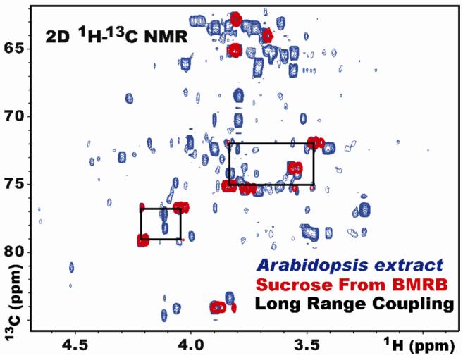
Two-dimensional ¹H-¹³C HSQC NMR spectrum of sucrose from the BMRB (red) overlaid onto an aqueous whole-plant extract from Arabidopsis thaliana (blue). Black boxes indicate long-range proton carbon couplings used to validate the assignment.

Step 2: Concentration Reference Samples

Six equimolar mixtures of the identified metabolites (2 mM N=2, 5 mM N=2, and 10 mM N=2) were prepared as concentration reference samples (see Preparation of synthetic samples).

Step 3: Data Collection

All test samples and concentration reference samples were run as a block under identical acquisition parameters (see NMR Spectroscopy). The sample block was run twice to produce two technical replicates for each sample. To minimize experimental bias, a random number generator (www.radom.org) was used to determine the sample order. 1D ¹H and 2D ¹H-¹³C HSQC spectra were collected sequentially on each sample with custom macros written in-house.

Step 4: Calculation of Concentrations

For the error analysis study, two well-dispersed peaks in the ¹H-¹³C HSQC spectra were selected for each of the seven target metabolites. A standard curve was constructed for each metabolite by regressing absolute peak intensities from the concentration reference samples with their known concentrations (Figure 4). Standard curves were averaged across the technical replicates (N=4, two block replicates and two sample replicates), and the resulting regression coefficients were used to predict metabolite concentrations in the test samples. Concentration estimates were also averaged across technical replicates (N=4, two block replicates, and two peaks were selected from each molecule) to produce a final predicted concentration for each metabolite. Identical procedures were used to estimate concentrations from both 1D and 2D NMR data. Proton chemical shifts used in the 1D ¹H analysis were those identified from the positions of 2D ¹H-¹³C HSQC cross peaks. These shifts were hand-verified to ensure that the correct resonance was selected. Some minor adjustments to the HSQC-based chemical shifts (± 0.005 ppm) were necessary because of the higher resolution of the 1D ¹H spectra. Chemical shift translation was done with custom scripts written in R.

Figure 4.

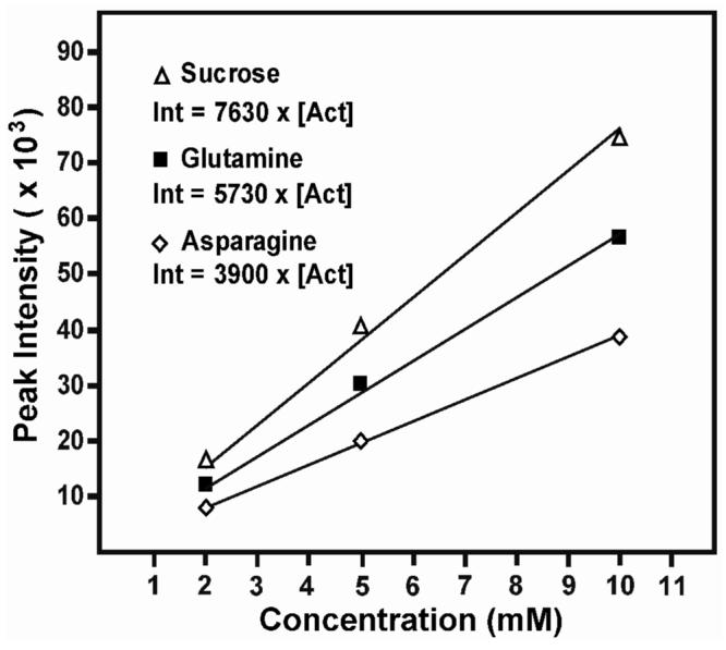
Two-dimensional ¹H-¹³C HSQC NMR peak intensities for three metabolites in the concentration reference samples plotted as a function of known concentration. The concentration of metabolites in the test samples were calculated from the best fit regression lines of the concentration reference samples.

Step 4 (alternative): Normalized Calculation of Concentrations

All of the samples used in this study contained 5mM HEPES as an internal standard. An alternative strategy used for calculating concentrations was to normalize all observed intensities to the average signal from the two dispersed HEPES peaks. Standard curves were then constructed with the HEPES normalized intensities, and concentrations were predicted in the same manner as described above. This method corrects for any changes in the NMR sensitivity between experiments and allows standards to be collected at a different time from the test samples. Metabolite concentration estimates for the biological extracts were carried out in this manner, and all well-dispersed peaks were used in the calculations. Chemical shifts and raw intensities of peaks used for quantification are provided as text files in the supplementary materials.

Data Availability

A detailed description of the metabolite identification process, assignment criteria, chemical shifts of assigned metabolites, a metabolite assignment tutorial, processed NMR data, and R functions used for automatic peak assignment, quantification, and regression analysis are available as downloadable files from the NMRFAM website at http://www.nmrfam.wisc.edu/Software/FMQ_data/.

RESULTS

Regression and Error Analyses

One hundred sixty-eight NMR-based concentration estimates were made from NMR spectra of the 24 synthetic mixtures. Each estimate was regressed against the known concentration of the metabolite (Figure 5). Parallel regressions of 2D ¹H-¹³C HSQC and 1D ¹H NMR measurements indicated that the 1D estimates were considerably noisier than the 2D estimates (r² = 0.88 versus r² = 0.99). In addition, regression slopes indicated that the 2D ¹H-¹³C HSQC estimates were precise (slope = 0.97; theoretical slope = 1), whereas the 1D ¹H-based data underestimated concentration (slope = 0.71; theoretical slope = 1). Error estimates calculated from the divergence of observed from actual concentrations indicated that the HSQC-based method averaged 2.7 % error with a maximum of 10.3 %, while the 1D ¹H analysis averaged 16.2 % error with a maximum of 44.5 % (Supplementary Figure 2). This error translates to an average (root mean square) accuracy of 0.6 mM for the 2D and 3.5 mM accuracy for 1D estimates.

Figure 5.

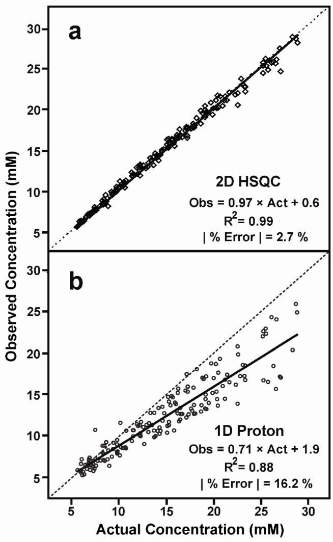
(a) Concentration estimates (N = 168) based on two-dimensional ¹H-¹³C HSQC and (b) one-dimensional ¹H NMR data. Estimates are plotted as a function of the known concentration of metabolites in synthetic mixtures. Dotted lines indicate the ideal regression (slope = 1) and the solid lines indicate the best fit regression.

Quantification of biological extracts

Fifty metabolites (excluding HEPES and MES) were identified in high resolution spectra of the three biological extracts. Forty of these were observed in Arabidopsis, thirty-seven were seen in alfalfa sprouts, and forty-one were present in yeast extracts. These metabolites represented, respectively: 81%, 81%, and 86% of the observed peaks in the Arabidopsis, alfalfa, and yeast extracts (Supplementary Table 2). Of the 50 observed metabolites, 41 (82%) could be quantified in automated fashion from 12-min 2D ¹H-¹³C data acquisitions. Observed concentrations, as measured in the NMR tube, ranged from 230 mM to as little as 40 μM (Supplementary Table 3). Metabolite concentrations below 1 mM should be treated with caution because they are below the limit of our measured error. Half of the metabolites seen in high resolution ¹H-¹³C NMR had concentrations lower than 4 mM and metabolites observed in the three tissues were distributed proportionally to the inverse of concentration (Figure 6).

Figure 6.

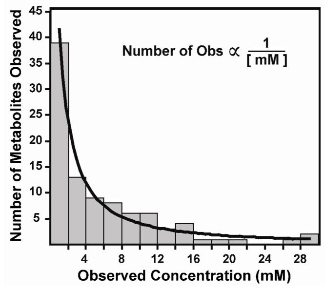
Number of observed metabolites in Arabidopsis, Medicago, and Saccharomyces extracts as a function of observed concentration (mM in the NMR tube; N=94). Bars indicate the total number of metabolite occurrences in the three extracts within consecutive 2 mM windows, and the regression line indicates the best-fit power regression (y = 42 × x ^-1.36, r² = 0.86). The internal standard (HEPES; N = 3), overlapped metabolites (acetate, lactate, and putrescine; N = 9) and nine metabolites with concentrations over 30 mM were excluded from the analysis. Metabolites observed in high resolution ¹H-¹³C HSQC spectra that were too dilute for FMQ by NMR (N = 13) were included with the quantifiable metabolites in the 0-2 mM bar. A complete list of all observed concentrations is provided in Supplementary Table 1.

Factors influencing quantification

It should be noted that most metabolite concentrations were predicted well beyond the range of the standard intensity versus concentration curves. In an earlier trial of this experiment, we found that higher standard concentrations (>10 mM for each metabolite) influenced the sensitivity of the probe and produced nonlinear calibration curves. When included in an analysis, the nonlinear standards caused a systematic underestimate of concentration and greater technical error (data not shown). It should also be noted that the standards data must be collected at multiple concentrations for accurate quantification. Multidimensional peak intensities are influenced by a range of variables (uneven excitation, multiple relaxation pathways, etc.) that change the scaling factors for individual peaks from different metabolites (Figure 4). Our data show that calculating concentrations from three standard concentrations (2 mM, 5 mM, and 10 mM) is sufficient for estimating concentrations between 1 mM and 30 mM.

We recognize that quantitative estimates are influenced by any variable that affects spectrometer sensitivity (primarily salt concentration and NMR line shape). HEPES (5 mM) was included in all the samples to act as an internal control for these variables. HEPES is a convenient choice for 2D ¹H-¹³C NMR studies, because it is a pH indicator and has several well dispersed peaks (Fig. 1). An additional benefit of HEPES normalization is that it allows standard curves generated for one study to be used in others, provided that all of the NMR instrument settings are identical. However, we found that HEPES normalization in the synthetic samples led to greater (10.2%) technical error (Supplementary Figure 2). In our experience, accurate quantification (<3% error) requires measurements of absolute peak intensities referenced to concentration standards collected at the same time as the test samples.

Sample Size Requirements for Fast Quantification

Fast 2D ¹H-¹³C NMR quantification requires a substantial amount of starting material. In this study, we extracted 400 mg of dry weight tissue per sample, used standard 5 mm NMR tubes, and collected data for 12 min. The sample requirement can be reduced to 200 mg by using 5 mm susceptibility matched NMR tubes (e.g. from Shigemi, Inc), which require smaller volumes and at the same concentration provide nearly the same signal-to-noise. Smaller amounts of starting material will result in loss of information about metabolites present below the detection threshold. The use of longer NMR data collection times can compensate for lower concentrations, but because NMR sensitivity scales with the square-root of the number of scans, this approach is limited.

DISCUSSION

Our data indicate that 2D ¹H-¹³C HSQC is superior to 1D ¹H NMR for quantitative analyses of complex mixtures. Although lower error estimates (∼1%) have been reported for 1D ¹H NMR analyses,^17-19 these studies have been limited to well dispersed peaks. One-dimensional ¹H NMR spectra of unfractionated biological extracts contain hundreds of overlapping resonances. Our analysis indicates that peak overlap considerably increases technical error.

We believe that the error estimates reported here represent the practical limit of quantitative precision for 1D ¹H NMR based metabolomics. Our synthetic mixtures included only 26 metabolites, and we had the luxury of knowing the exact chemical shifts of every molecule from 2D ¹H-¹³C HSQC spectra. NMR-based analyses of real biological samples must contend with >50 observable compounds with ambiguous resonance assignments and larger variations in chemical shift than our synthetic mixtures. Although these present serious obstacles for 1D ¹H NMR analysis, they can be overcome using the 2D ¹H-¹³C NMR protocol we introduce here.

FMQ by NMR requires that target metabolites be identified prior to quantitative analysis. Although the identification of metabolites is laborious, it enables well controlled quantitative analyses to be based on intensities of minimally overlapping peaks. Our experimental method and guidelines for reducing NMR acquisition times should make quantitative metabolite analyses feasible for biological studies in which 200-400 mg (weight of dry tissue prior to extraction) samples can be obtained.

REFERENCES

- (1).Pauli GF, Jaki BU, Lankin DC. J Nat Prod. 2005;68:133–149. doi: 10.1021/np0497301. [DOI] [PubMed] [Google Scholar]
- (2).Radda GK, Seeley PJ. Annu Rev Physiol. 1979;41:749–769. doi: 10.1146/annurev.ph.41.030179.003533. [DOI] [PubMed] [Google Scholar]
- (3).Lindon JC, Nicholson JK, Holmes E, Everett JR. Concepts in Magnetic Resonance. 2000;12:289–320. [Google Scholar]
- (4).Lindon JC, Holmes E, Nicholson JK. Progress in Nuclear Magnetic Resonance Spectroscopy. 2001;39:1–40. [Google Scholar]
- (5).Holmes E, Cloarec O, Nicholson JK. Journal of Proteome Res. 2006;5:1313–1320. doi: 10.1021/pr050399w. [DOI] [PubMed] [Google Scholar]
- (6).Dumas ME, Maibaum EC, Teague C, Ueshima H, Zhou B, Lindon JC, Nicholson JK, Stamler J, Elliott P, Chan Q, Holmes E. Anal Chem. 2006;78:2199–2208. doi: 10.1021/ac0517085. [DOI] [PMC free article] [PubMed] [Google Scholar]
- (7).Weljie AM, Newton J, Mercier P, Carlson E, Slupsky CM. Anal Chem. 2006;78:4430–4442. doi: 10.1021/ac060209g. [DOI] [PubMed] [Google Scholar]
- (8).Fan TWM. Progress in Nuclear Magnetic Resonance Spectroscopy. 1996;28:161–219. [Google Scholar]
- (9).Viant MR. Biochem.Biophys.Res.Commun. 2003;310:943–948. doi: 10.1016/j.bbrc.2003.09.092. [DOI] [PubMed] [Google Scholar]
- (10).Kikuchi J, Shinozaki K, Hirayama T. Plant Cell Physiol. 2004;45:1099–1104. doi: 10.1093/pcp/pch117. [DOI] [PubMed] [Google Scholar]
- (11).Fan TWM, Lane AN, Shenker M, Bartley JP, Crowley D, Higashi RM. Phytochemistry. 2001;57:209–221. doi: 10.1016/s0031-9422(01)00007-3. [DOI] [PubMed] [Google Scholar]
- (12).Seavey BR, Farr EA, Westler WM, Markley JL. J Biomol NMR. 1991;1:217–236. doi: 10.1007/BF01875516. [DOI] [PubMed] [Google Scholar]
- (13).Markley JL, Anderson ME, Cui Q, Eghbalnia HR, Lewis IA, Hegeman AD, Li J, Schulte CR, Sussman MR, Westler WM, Ulrich EL, Zolnai Z. Pac. Symp. Biocomput. 2007;12:157–168. [PubMed] [Google Scholar]
- (14).Wishart DS, Tzur D, Knox C, Eisner R, Guo AC, Young N, Cheng D, Jewell K, Arndt D, Sawhney S, Fung C, Nikolai L, Lewis M, Coutouly MA, Forsythe I, Tang P, Shrivastava S, Jeroncic K, Stothard P, Amegbey G, Block D, Hau DD, Wagner J, Miniaci J, Clements M, Gebremedhin M, Guo N, Zhang Y, Duggan GE, Macinnis GD, Weljie AM, Dowlatabadi R, Bamforth F, Clive D, Greiner R, Li L, Marrie T, Sykes BD, Vogel HJ, Querengesser L. Nucleic Acids Res. 2007;35:D521–526. doi: 10.1093/nar/gkl923. [DOI] [PMC free article] [PubMed] [Google Scholar]
- (15).Marashige T, Skoog F. Physiol. Plant. 1962;15:473–479. [Google Scholar]
- (16).Delaglio F, Grzesiek S, Vuister GW, Zhu G, Pfeifer J, Bax A. Journal of Biomolecular NMR. 1995;6:277–293. doi: 10.1007/BF00197809. [DOI] [PubMed] [Google Scholar]
- (17).Malz F, Jancke H. J Pharm Biomed Anal. 2005;38:813–823. doi: 10.1016/j.jpba.2005.01.043. [DOI] [PubMed] [Google Scholar]
- (18).Burton IW, Quilliam MA, Walter JA. Anal Chem. 2005;77:3123–3131. doi: 10.1021/ac048385h. [DOI] [PubMed] [Google Scholar]
- (19).Pinciroli V, Biancardi R, Visentin G, Rizzo V. Organic Process Research & Development. 2004;8:381–384. [Google Scholar]
Associated Data
This section collects any data citations, data availability statements, or supplementary materials included in this article.
Supplementary Materials
Data Availability Statement