The Evolutionary Rate of Duplicated Genes Under Concerted Evolution

Abstract

The effect of directional selection on the fixation process of a single mutation that spreads in a multigene family by gene conversion is investigated. A simple two-locus model with two alleles, A and a, is first considered in a random-mating diploid population with size N. There are four haplotypes, AA, Aa, aA, and aa, and selection works on the number of alleles A in a diplod (i = 0, 1, 2, 3, 4). Because gene conversion is allowed between the two loci, when the mutation rate is very low, either AA or aa will fix in the population eventually. We consider a situation where a single mutant, A, arises in one locus when a is fixed in both loci. Then, we derive the fixation probability analytically, and the fixation time is investigated by simulations. It is found that gene conversion has an effect to increase the “effective” population size, so that weak selection works more efficiently in a multigene family. With these results, we discuss the effect of gene conversion on the rate of molecular evolution in a multigene family undergoing concerted evolution. We also argue about the applicability of the theoretical results to models of multigene families with more than two loci.

THE evolutionary rate of a gene may be defined as the rate of nucleotide substitutions in a certain time period, say, per year or per generation (Zuckerkandl and Pauling 1965; Jukes and Cantor 1969). Theoretically, the rate is given by the product of the mutation rate (μ) and fixation probability (u). Under neutrality, it is well known that, in a random-mating population with N diploids, the neutral evolutionary rate is identical to the mutation rate, because on average 2Nμ mutations arise in the population every generation and each will fix in the population with probability u = 1/2N. When selection is active, the fixation probability is given by

(1)

where is the initial frequency of the mutant, that is, 1/2N (Kimura 1962).

Although the above theory is for a single-copy gene, fixations of mutations also occur in genes that belong to a multigene family. It is possible that a mutation spreads over all member genes of a multigene family when they undergo concerted evolution, a phenomenon that the copy members evolve in a concerted manner by exchanging their DNA sequences (Ohta 1980; Dover 1982; Arnheim 1983). A typical observation of concerted evolution is that the nucleotide sequence divergence between the copy members in the family is very low because of frequent exchanges of genetic information, while there is substantial divergence from the orthologous family in other species. This means that genetic variation within the family can “migrate” between different copies, and a certain allele eventually becomes fixed in the species. The accumulation of such fixations results in the difference between species.

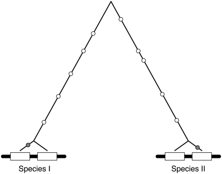
The purpose of this article is to investigate the fixation process of a mutation through the whole family members via gene conversion. Gene conversion between copy members should be the major mechanism to cause concerted evolution of small multigene families (Ohta 1983a; Li 1997), while both gene conversion and unequal crossing over should be working simultaneously in middle- and large-size families (Hillis et al. 1991; Gangloff et al. 1996). This article focuses on the rate of nucleotide substitutions (i.e., evolutionary rate) in duplicated genes (or a small multigene family) that are currently undergoing concerted evolution by gene conversion. Figure 1 shows a typical gene tree of a pair of duplicated genes in two species. It is supposed that the duplication event predates the speciation event; therefore, the two duplicated genes are present in both species. When concerted evolution is going on in the gene pairs of both species, the sequence similarity between the two duplicates should be low. Meanwhile, the accumulation of nucleotide substitutions over time makes a difference between the two species, which results in fixed nucleotide differences between the two species (open circles in Figure 1). When the mutant is in a transient phase to fixation (or extinction), it could appear as nucleotide variation between duplicated pairs within the same species (shaded circles in Figure 1). Theoretical aspects of such variation within a family have been extensively studied by Innan (2002, 2003a) and Teshima and Innan (2004).

Figure 1.—

Gene tree of a pair duplicated genes from two species. The two boxes represents the duplicated gene pair. The gene pairs are present in the two species, because the duplication event predates the speciation event. The duplicated gene pairs are still undergoing concerted evolution, so that the resultant gene tree of the four genes should look as illustrated: the paralogous gene pair in each species is more closely related than the orthologous pairs. The circles represent the mutations that occurred along the evolution of the four genes since the speciation event. The open circles are those fixed in each species, while the shaded ones are the variation between duplicated copies.

Although the process of interest is emphasized by comparing the sequences between two different species (Figure 1), each fixation event is a matter of population genetics, that is, an event that occurs in a single population. The process starts with an introduction of a new mutation in one of the copy members in the family. The fixation of the new allele in the whole family is achieved when all individuals in the population have the new allele at all loci. The process involves “migrations” of alleles from one copy to another, and gene conversion is the mechanism to cause interlocus migration. To develop a solid mathematical framework of this complicated fixation process, we use the diffusion method, a classic mathematical approach in population genetics, with a simple two-locus model. We here obtain analytical results for the fixation probability of a mutation, and the fixation time is investigated by simulations. Walsh (1985) provided an analytical expression for the fixation probability with the assumption of a low gene conversion rate. Our diffusion treatment enables us to derive a general formula that is applicable to any gene conversion rate (see below for details).

THEORY

Consider a two-locus model in a random-mating diploid population with size N. Only two alleles (A and a) are allowed for the two loci in total, so that there are four gametes (haplotypes), AA, Aa, aA, and aa, where the two characters represent the allelic states at the first and second loci. The model is essentially the same as that of Innan (2002). Let x₁, x₂, x₃, and x₄ be the frequencies of the four gametes, AA, Aa, aA, and aa, respectively. Because x₄ = 1 – (x₁ + x₂ + x₃), the behavior of the frequencies of the four gametes can be described in a three-dimensional diffusion process within K, where K = {0 ≤ x₁ ≤ x₁ + x₂ ≤ x₁ + x₂ + x₃ ≤ 1}. Symmetrical gene conversion occurs to homogenize the variation between the two loci at rate c per generation; that is, Aa and aA change to AA at rate c and to aa at the same rate. The recombination rate between the two loci is denoted by r. The population gene conversion and recombination parameters are defined as C = 4Nc and R = 4Nr, respectively.

The model involves selection that favors (or disfavors) A to a. In this diploid system, we assume that selection works on the number of the preferred alleles in each diploid, so that the fitness of diploids with i A alleles (i = 0, 1, 2, 3, 4) is given by

(2)

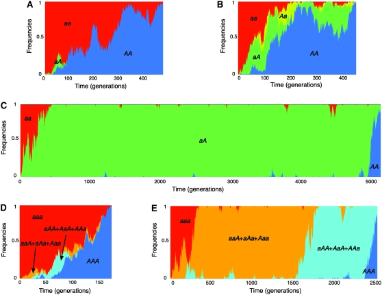
Under this framework, we are interested in the process that allele A spreads in the population under our two-locus system. For an intuitive understanding of the process of interest, Figure 2 shows simulated behaviors of the frequencies of the four haplotypes along the fixation of allele A, given the initial state where haplotype aa (represented by the red parts in Figure 2) is fixed. At time 0, a single haplotype aA (represented in green) is introduced, and the trajectories of the frequencies of the four haplotypes are simulated until allele A becomes fixed in the population; that is, all individuals are homozygotes of AA (represented in blue). To demonstrate the point, A is assumed to be advantageous over a. See the next section for details about the simulations. Figure 2A is a single realization of the fixation process of A when there is no recombination between the two loci, and a relatively high gene conversion rate is assumed. Along the increase of aA, gene conversion transfers A from the second locus to the first locus, creating the most advantageous haplotype, AA. Then, the population is completely replaced by A when AA is fixed. The pattern is similar with frequent recombination except that the process involves Aa that is produced by recombination between AA and aa (Figure 2B). The fixation process takes a much longer time when the gene conversion rate is very low (Figure 2C). The fixations of A at the two loci occur as two essentially independent events: A is fixed first at the second locus and there is a long waiting time for the second fixation at the first locus because of a very low gene conversion rate. Walsh's (1985) theory is based on this situation of a weak-conversion limit; he assumed that the fixation of A at each locus occurs in a very short time, so that the process of the spread of A over all copy members can be handled as a locus-by-locus process. Note that such a locus-by-locus fixation assumption holds when there are more than two loci. For example, in a three-locus model, the fixation of A could occur locus by locus for a low gene conversion rate as shown in Figure 2E. Meanwhile, when the gene conversion rate is high, the fixation of A seems to occur simultaneously in the three loci (Figure 2D). In this article, we are interested in the general case, including cases where the gene conversion rate is relatively high so that the fixation of A at each locus and the interlocus spread occur simultaneously. Therefore, any value of the gene conversion rate can be applied to the following derivations.

Figure 2.—

(A–D) Typical trajectories of the frequencies of the four haplotypes, AA, Aa, aA, and aa in a two-locus model, represented by the blue, green, yellow, and red parts. The trajectories were obtained by simulations with a random-mating diploid population with size 100, where s = 0.01 is assumed. (A) c = 0.01 and r = 0. (B) c = 0.01 and r = 0.1. (C) c = 0.0001 and r = 0. (D and E) Typical trajectories of haplotype frequencies in a three-locus model. (D) c = 0.01 and r = 0. (E) c = 0.0001 and r = 0.

In our model, the expected frequencies of the four haplotypes in the next generation (, , , ) are given by

(3)

(4)

(5)

(6)

where D = x₁x₄ – x₂x₃ and M_i is given by

The recursion equations are almost identical to those used in Innan (2003b) except for the selection terms (the last term in each equation). Therefore, the expected changes of the frequencies in a single generation are given by

(7)

(8)

(9)

(10)

For our purpose, it may be convenient to transfer Φ: {x₁, x₂, x₃} ↦ {p, q, D}, where

(11)

This transformation was first introduced by Ohta and Kimura (1969) and is useful in models of duplicated genes with gene conversion (Innan 2002, 2003b). Then, because

(12)

(13)

(14)

we have

(15)

(16)

(17)

where

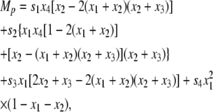(18)

(19)

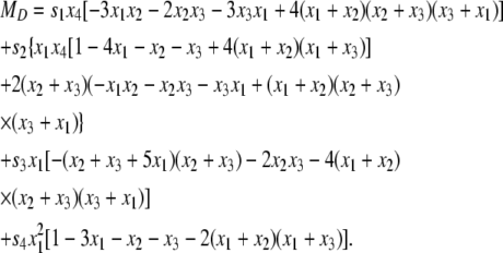(20)

Then, the diffusion process {p(t), q(t), D(t): t ≥ 0} in Φ(K) is governed by a generator

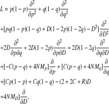(21)

where time is measured in units of 4N generations. This operator is almost identical to that used in Innan (2003b) except for the selection terms. See Kimura (1964) for more details about derivation.

When we count the degree of terms by the sum of degrees in p, q, and twice that of D (e.g., the degree of pqD is 1 + 1 + 2 = 4), in general, M_p and M_q involve up to the fifth-degree terms, which makes the computation very difficult. To overcome this problem, it is extremely important to reduce the degree of terms in the diffusion operator (21). We found that it is possible to reduce the degrees of M_p and M_q if we put the conditions s₃ = −3s₁ + 3s₂ and s₄ = −8s₁ + 6s₂. With these conditions, M_p and M_q involve only up to the third-degree terms, making the following mathematical treatment feasible. To do so, we need to reparameterize the selection coefficients by two parameters, s and h:

(22)

h is a parameter to summarize the dominance effect as illustrated in Figure 3. When h = , the effect of selection is additive. The function of s_i is concave when h < , while convex when . With this expression of the selection coefficients, M_p, M_q, and M_D can be given by relatively simple formulas:

(23)

(24)

(25)

Figure 3.—

Selection coefficients of the five gametes when the dominance effect is incorporated by Equation 22. The solid line shows the selection coefficients when the effect is additive. (A) h = 0.2, representing a case where A is recessive. (B) h = 0.5; that is, the selection effect is completely additive. (C) h = 0.8, representing a case where A is dominant.

Here, we attempt to obtain u(p, q, D), the fixation probability of allele A with initial condition (p, q, D). u(p, q, D) satisfies the following partial differential equation:

(26)

As long as c > 0, the process ends when either A or a fixes in both of the two loci. In other words, the exit boundaries are (p, q, D) = (1, 1, 0) and (0, 0, 0), and we have u(1, 1, 0) = 1 and u(0, 0, 0) = 0. See appendix a for details about the other boundary conditions, ∂Φ(K) – {(1, 1, 0), (0, 0, 0)}.

Because it may be extremely difficult to obtain a closed-form solution to u(p, q, D) directly from Equation 26, as an alternative way, we consider ψ_ℓ,m,n = E[p^ℓ(t)q^m(t)Dⁿ(t)]. Because (p, q, D) = (1, 1, 0) and (0, 0, 0) are the exit boundaries, in the limit there is no probability mass except for these two boundaries. Then, we have

(27)

therefore, assuming the selection coefficient is not very large, u(p, q, D) should be written as a perturbative series in 4Ns:

(28)

To obtain the coefficients f_j(p, q, D), in the following, we first consider ψ_1,0,0. The moments can be represented by perturbative series in 4Ns:

(29)

Then, after some calculations (appendix a), we have

(30)

(31)

where is the mean initial frequency of allele A, which is given by . is terms that decay with time, and . Therefore, it does not play an important role in the following derivation, which focuses on the case of .

In a similar way, we are able to obtain the expectations of other moments (appendix b). Then, considering all moments, up to the second order of 4Ns in Equation 28, we have the fixation probability of a newly arisen mutation in this two-locus system as ,

(32)

when h = (the general form is shown in appendix b).

Here, it is interesting to note that Equation 28 has an extremely similar form to the Taylor series expansion of the fixation probability as a function of 2Ns, which is given by

(33)

(34)

The first terms of Equations 32 and 34 are identical. For the second term, the coefficients of are 2Ns and 4Ns for and , respectively, indicating the coefficient might be given by 2nNs for . A similar logic might hold for the third order: the coefficients of are (2Ns)² and (4Ns)², suggesting the coefficient for should be (2nNs)². Thus, the comparison of Equations 32 and 34 enables us to suspect that is given by

(35)

If so, it is straightforward to expect that has a closed form,

(36)

and is given by

(37)

Actually, Equation 37 satisfies the partial differential Equation 26, u(1, 1, 0) = 1, u(0, 0, 0) = 0, and u(p, q, D)|_{∂Φ(K)–{(1, 1, 0),(0, 0, 0)}} < ∞. Note that, from this equation, we can derive Walsh's result (Equation 8 in Walsh 1985) with the condition of low gene conversion rate. Furthermore, Equation 36 should be the solution of the fixation probability for similar models with more than two loci. This equation is also in agreement with Walsh (1985) at the low conversion limit. Equations 36 and 37 are also consistent with the result of Nagylaki and Petes (1982), who obtained the fixation probability under neutrality .

It should be noted that all terms involving the gene conversion and recombination rates are canceled out in the above derivation, so that the fixation probability is given by a function of Ns and . Equation 36 is equivalent to the fixation probability of a single-copy gene in a random-mating population with size nN, indicating that allelic migration between copy members by gene conversion has an effect to increase the effective population. An intuitive understanding is that this effect holds as long as c > 0. Recombination works to enhance the homogenizing effect of gene conversion (Innan 2002). Therefore, as long as the gene conversion rate has no effect, the fixation probability should be independent of the recombination rate.

SIMULATIONS

Two-locus model:

Forward simulations were performed to check if our predicted Equation 37 works. The simulations follow the standard Wright–Fisher model. A random-mating diploid population with size N = 100 is considered. Time 0 is set such that a single aA haplotype arises in the population where aa is fixed; therefore, the initial state of haplotype frequencies is . Following the recursion (3)–(6), a single run of forward simulation is continued until one allele is fixed in the two loci; that is, (x₁, x₂, x₃, x₄) = (0, 0, 0, 1) or (1, 0, 0, 0). For each parameter set, 10⁷ replications of simulations were performed and the proportion of the fixation events of allele A was obtained.

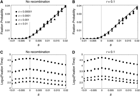
Figure 4 summarizes the simulation results, showing that Equation 37 is in excellent agreement with the simulations for a wide range of the gene conversion rates (c = 0.00001–0.01) when there is no recombination (Figure 4A) and when the recombination rate is very high (Figure 4B). It is indicated that Equation 37 could be the solution to the fixation probability in the two-locus model. As Equation 37 indicates, the probability is independent of the gene conversion rate or recombination rate. Almost identical simulation results were obtained for other recombination rates (not shown).

Figure 4.—

Fixation probability and fixation time in the two-locus model. (A and B) Simulation results for the fixation probability when the recombination rate is 0 and 0.1, respectively. The shaded lines represents the theoretical result from Equation 37. (C and D) Simulation results for the fixation time when the recombination rate is 0 and 0.1, respectively. The results are based on simulations with 10⁷ replications for each parameter set.

The simulations also demonstrate that the fixation time is given by a complicated function of N, c, s, and r, as shown in Figure 4. When c is very small, the fixation time dramatically increases as the gene conversion rate decreases (Figure 4, C and D). This is because a typical fixation occurs such that a new mutation first fixes in one locus and waits for the fixation in the second locus. This waiting time is very long and determined by the amount of gene flow from the first to the second locus and the rate of their fixation in the second locus. The gene conversion rate is negatively correlated with the former, while the selection intensity determines the latter. Selection also has a negative correlation with the time of fixation in each locus. The fixation time is longer with a larger recombination rate.

When c is so large that there are substantial exchanges between the two loci, it seems that selection is the dominant factor to determine the fixation time, because the fixation occurs almost in a single gene pool with size 4N. As the absolute value of s increases, the mean fixation time decreases, and the fixation time could be largest when neutral. This pattern is similar to that in the standard single-locus system (Crow and Kimura 1970), except that the expected fixation times for s and –s are identical in the standard single-locus system, but not in our two-locus model (Figure 4, C and D).

More loci:

The simulations in the two-locus model demonstrated that Equation 36 works very well when n = 2. The model is further extended to the case of n = 3 to check the performance of Equation 36. The three-locus model considers three tandemly arrayed genes, I, II, and III. The recombination rates between I and II and between II and III are assumed to be the same (r). It is also assumed that symmetrical gene conversion occurs between all three gene pairs at the same rate, c.

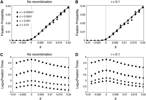
The results in the three-locus model are very similar to those for the two-locus model. The fixation probability seems to follow Equation 36 regardless of the gene conversion or recombination rates (Figure 5, A and B). The fixation time depends on the gene conversion and recombination rates and selection coefficient, and their effects on the fixation time are similar to those in the two-locus model.

Figure 5.—

Fixation probability and fixation time in the three-locus model. (A and B) Simulation results for the fixation probability when the recombination rate is 0 and 0.1, respectively. The number of replications is 10⁷ for each parameter set. The shaded lines represent the theoretical result from Equation 35 with n = 3. (C and D) Simulation results for the fixation time when the recombination rate is 0. Data for the mean fixation time when s = −0.01 are missing because the fixation event is so rare that we were not able to obtain reliable mean values.

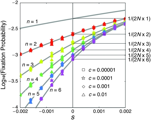
Additional simulations show that Equation 36 is in excellent agreement with the simulation results for n up to 6 (Figure 6). A narrow range of s is investigated here because the effect of n is primarily observed when selection is very weak (see also Figure 7A).

Figure 6.—

Fixation probability for n = {1, 2, 3, 4, 5, 6} predicted by Equation 36 with simulation results for c = 0.00001, 0.0001, 0.001, and 0.01. The number of replications is 10⁷ for each parameter set.

Figure 7.—

(A) Fixation probability for n = {1, 2, 3, 4} predicted by Equation 36. N = 100 is assumed so that the probability of the neutral case is given by 1/(2nN) = 1/(200n). (B) Substitution rate for n = {1, 2, 3, 4} from Equation 38. The substitution rate is measured such that the rate is 1 under neutrality (note that the substitution rate per site per generation is identical to the mutation rate for any n).

Biased gene conversion:

It is known that mismatch repair following gene conversion likely occurs with bias, that is, biased gene conversion (Galtier 2003; Marais 2003). Gene conversion could favor particular alleles over others, usually GC over AT base pairs. Because it is extremely difficult to incorporate biased gene conversion in the above derivation, we investigate its effect on the fixation probability by simulations. Following Walsh (1985), the degree of bias in gene conversion is denoted by α, such that the recursions of (x₁, x₂, x₃, x₄) are rewritten as

In this setting, α represents the proportion of gene conversion. When α = 0.5, there is no bias and these recursions are identical to (3)–(6). The bias is toward A if α > 0.5. Figure 8 shows that the fixation probability of A is elevated for α > 0.5 (red) and vice versa (blue). The effect of biased gene conversion is especially large when the gene conversion rate is high (Figure 8B). When the gene conversion rate is low, the results are in agreement with Walsh (1985), who suggested that the effect of biased gene conversion would be minor unless the selection intensity is very small.

Figure 8.—

(A and B) Effect of biased gene conversion on the fixation probability in the two-locus model. A total of 10⁷ replications of simulations were carried out for each parameter set.

DISCUSSION

The fixation process that a mutation spreads in a multigene family by gene conversion is investigated by theory and simulations. By obtaining the coefficients of moments of 4Ns of the fixation probability (Equation 28), we suspected that the closed form of the probability might be given by Equation 37 in the two-locus model, and the results of computer simulations support this. It is found that the fixation probability is given by a function of N and s and independent of the gene conversion (c) and recombination rates (r). The fixation time is given by a complicated function of N, s, c, and r. It is demonstrated that selection could be the dominant factor to determine the fixation time when c is large, while for a small c, both s and c play the major roles.

Ohta (1983b) discussed the fixation time of a neutral mutant by computing the decay rate of genetic identity (identity coefficient in her terminology). In our analysis of the fixation probability, we focus on the moments ψ_ℓ,0,0(ℓ ≥ 1). As shown in appendix b, the derivation of the moments involves the eigenvalues of matrices. Up to the second-degree moments in the 0th order of 4Ns, there are five nonzero eigenvalues involved, which are −2C, λ₁, λ₂, λ₃, and λ₄. Among them, the largest is always λ₂ (see appendix c), and this value corresponds to Ohta's decay rate of genetic identity.

We further extended the situation to models with more than two loci. The equation for the fixation probability given by (37) is so simple that we might expect that the fixation probability in the n-locus model may follow a similar form, that is, Equation 36. As expected, simulations showed that Equation 36 works very well in the models with up to n = 6 (Figure 6). It is suggested that Equation 36 might work for any positive integer n. Our theoretical results for the fixation probability suggest that gene conversion causes migrations between loci; therefore, it can be considered that the “effective” population size is increased because a single mutant has to be fixed in a gene pool of size 2nN. As a consequence, the initial frequency of the single mutant in the whole gene pool is smaller when n is large. This effect is well observed when s is small so that the relative contribution of the initial frequency to the fixation probability is large (Figure 6). Note that this effect is small for large Ns, where the fixation probability is almost independent of the initial frequency (approximately given by 2s).

It is worth pointing out that the expression (37) also appears in a problem in a subdivided population. Maruyama (1971) obtained the identical formula as the fixation probability of a mutant under genic selection, where the mutant spreads over the whole population that consists of n subpopulations, whose effective sizes are N for each. It is remarkable that the expression does not depend on the migration pattern, as long as the population sizes of each subpopulation are maintained. It is straightforward to show that the n-unlinked locus version of the generator (21) is identical to the generator of the process of a n-island model when the migration rates between subpopulations are given by C. Our expression (37) is supported by Maruyama's solution when R = ∞.

Our theoretical results have interesting implications on the evolutionary rate of duplicated genes. In the n-locus model, Equation 36 gives the fixation probability of a newly arisen mutation, which appears at rate 2nNμ per generation per population. Hence, the substitution rate can be given by

(38)

Figure 7B shows the substitution rate as a function of s for n = {1, 2, 3, 4}. It is obvious that this rate is μ under neutrality for any n, which is in agreement with Nagylaki and Petes (1982). This is also consistent with the neutral theory of molecular evolution (Kimura 1983). When s ≠ 0, selection works more efficiently in a larger gene family: the substitution rate of a beneficial mutation is higher for a larger family, while that of deleterious mutation is lower. Thus, it seems that having more copies in a family could enhance the action of directional selection, as long as there are exchanges of genetic materials among them. In other words, the action of weak selection would be more emphasized in a multigene family with a larger n.

Our theory predicts that the evolutionary rate at synonymous sites may be not be very different between a single-copy gene and a multigene family assuming μ is the same and synonymous sites are under very weak selection. This should not hold for the rate at nonsynonymous sites. It would be faster in a multigene family, if many sites are subject to positive selection. On the other hand, the nonsynonymous substitution rate in a multigene family may be slower if it is under the pressure of strong negative selection. This prediction may well explain a recent report, which demonstrated that the substitution rate at nonsynonymous sites is accelerated in a concerted gene cluster in Caenorhabditis elegans and its relatives (Thomas 2006). In this gene family, the effect of positive selection could be enhanced by exchanging among the members, as discussed by the author. It is indicated that gene conversion in a multigene family plays an important role in adaptive evolution, because beneficial mutations can be shared by the member genes in the family.

APPENDIX A: ARGUMENTS ON THE BOUNDARY CONDITION

This article includes appendixes a–c, which requires relatively high background in the diffusion theory. Therefore, we proceed along with two standard introductory textbooks (Morse and Feshbach 1953; Oksendal 2003), which have been commonly cited in theoretical literature in population genetics.

To address the boundary condition, it is convenient to consider the diffusion process {x₁(t), x₂(t), x₃(t): t ≥ 0} in K. The fixation probability u(x₁, x₂, x₃) satisfies the elliptic partial differential equation

where v is the drift term of the diffusion process (see appendix b for details). Note that the generator degenerates over ∂K. Since (x₁, x₂, x₃) = (1, 0, 0) and (0, 0, 0) are the exit boundaries, we put the Dirichlet-type conditions: u(1, 0, 0) = 1 and u(0, 0, 0) = 0 (Morse and Feshbach 1953). However, it is obvious that the other part S = ∂K – {(1, 0, 0), (0, 0, 0)} does not follow the standard types of boundary conditions such as the Dirichlet and Neumann types (Oleinik and Radkevic 1973).

For S = ∂K – {(1, 0, 0), (0, 0, 0)}, considering the fixation process in a population, it is reasonable to put u|_S = finite, where “finite” represents terms that do not depend on coordinates, which are normal to the boundary and bounded within (0, 1). These conditions reflect the fact that there should be finite probability of fixation when a population evolves from an arbitrary point in S. For example, consider a point (ɛ, c₂, c₃) ∈ K, which is close to the x₁ = 0 surface when ɛ is small. We may expand u by , where f_j(c₂, c₃) is an arbitrary function of c₂ and c₃ (see p. 374 in Morse and Feshbach 1953). To keep u(ɛ, c₂, c₃) finite with , we have to set f_j(c₂, c₃) = 0 (j < 0). Subsequently, we have . The solution (36) satisfies these conditions: and . This kind of argument on the boundary condition is commonly made in the literature, where the fixation time in the one-dimensional diffusion model is considered (e.g., Kimura and Ohta 1969).

APPENDIX B: DERIVATION OF THE MOMENTS

The diffusion process governed by the generator (21) is represented by a system of stochastic differential equations,

(B1)

(Oksendal 2003), where p = ^T(p, q, D) and σ is given such that σ^Tσ is the 4N times covariance matrix of p (Mano 2007). b is a vector of mutually independent Brownian motions, and

(Mano 2007). Taking the expectation of (B1), we have the ordinary differential equation for the moments ψ_1,0,0, ψ_0,1,0, ψ_0,0,1. For other moments, by applying the Itô formula to functions p^ℓq^mDⁿ(ℓ, m, n = 0, 1, 2, …), we have

(B2)

(see p. 48 in Oksendal 2003). Substituting (B1) into (B2) and taking the expectation, we have the ordinary differential equations for other moments (below).

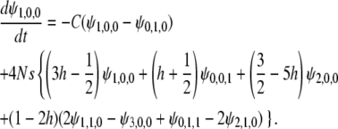
For ψ_1,0,0, we have

or

(B3)

Substituting (29) into Equation B3, we have ordinary differential equations for each order of the perturbation (see p. 1001 in Morse and Feshbach 1953). For the 0th order in 4Ns, we have

with the initial condition . For the i(≥ 1)th order, we have

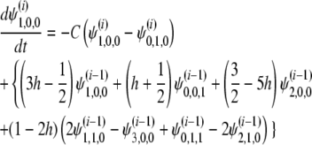with the initial condition ψ.

Let the Laplace transform of be . For the first-degree moments, we have

(B4)

where

(B5)

and E is the unit matrix. Also,

(B6)

(B7)

For the second-degree moments, we have

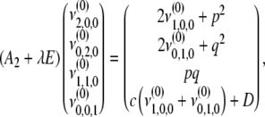(B8)

where

For the third-degree moments, we have

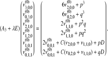(B9)

where

Solving (B4), we have

(B10)

where . Solving (B6) and (B7) with (B4), (B8), and (B9), we have

(B11)

where λ_i(< 0)(i = 1, 2, …, 10) are eigenvalues of A₂(i = 1, 2, 3, 4) and A₃(i = 5, …, 10), whose explicit forms are discussed in appendix c. a_i are polynomials of p, q, D, R, C, h. Applying the inverse Laplace transformation to (B10) and (B11), we obtain

(B12)

(B13)

where represents terms that decay with . Thus, up to the first order in 4Ns, we have

(B14)

APPENDIX C: EIGENVALUES

The two eigenvalues of A₁ are 0 and −2C. The four eigenvalues of A₂ are λ₁ = −2(1 + C) and the three roots of a cubic equation

(C1)

where S = λ + 2(1 + C). This is the same equation as that obtained by Ohta (1983b), where x in her Equation 4 is replaced by 4Nλ + 1. Let λ₂, λ₃, λ₄ be the three roots and assume λ₂ is the largest one. We have

where

Note that the largest eigenvalue of the five nonzero eigenvalues (−2C, λ₁, λ₂, λ₃, and λ₄) is always λ₂. This is clear from the cubic equation (C1), where we have λ₂ + 2(1 + C) ≥ 2 and λ₂ ≥ −2C > λ₁ = −2C – 2 because the left side of this equation is −4C²R ≤ 0 at S = 2.

The six eigenvalues of A₃ can also be computed by a similar method. The results are too complicated to show here and are available upon request.

References

- Arnheim, N., 1983. Concerted evolution of multigene families, pp. 38–61 in Evolution of Genes and Proteins, edited by M. Nei and R. K. Koehn. Sinauer Associates, Sunderland, MA.
- Crow, J. F., and M. Kimura, 1970. An Introduction to Population Genetics Theory. Harper & Row, New York.
- Dover, G., 1982. Molecular drive: a cohesive mode of species evolution. Nature 299 111–117. [DOI] [PubMed] [Google Scholar]
- Galtier, N., 2003. Gene conversion drives GC content evolution in mammalian histones. Trends Genet. 19 65–68. [DOI] [PubMed] [Google Scholar]
- Gangloff, S., H. Zou and R. Rothstein, 1996. Gene conversion plays the major role in controlling the stability of large tandem repeats in yeast. EMBO J. 15 1715–1725. [PMC free article] [PubMed] [Google Scholar]
- Hillis, D. M., C. Moritz, C. A. Porter and R. J. Baker, 1991. Evidence for biased gene conversion in concerted evolution of ribosomal dna. Science 251 308–310. [DOI] [PubMed] [Google Scholar]
- Innan, H., 2002. A method for estimating the mutation, gene conversion and recombination parameters in small multigene families. Genetics 161 865–872. [DOI] [PMC free article] [PubMed] [Google Scholar]
- Innan, H., 2003. a The coalescent and infinite-site model of a small multigene family. Genetics 163 803–810. [DOI] [PMC free article] [PubMed] [Google Scholar]
- Innan, H., 2003. b A two-locus gene conversion model with selection and its application to the human RHCE and RHD genes. Proc. Natl. Acad. Sci. USA 100 8793–8798. [DOI] [PMC free article] [PubMed] [Google Scholar]
- Jukes, T. H., and D. R. Cantor, 1969. Evolution of protein molecules, pp. 21–132 in Mammalian Protein Metabolism, edited by H. N. Munro. Academic Press, New York.
- Kimura, M., 1962. On the probability of fixation of mutant genes in a population. Genetics 47 713–719. [DOI] [PMC free article] [PubMed] [Google Scholar]
- Kimura, M., 1964. Diffusion models in population genetics. J. Appl. Probab. 1 177–232. [Google Scholar]
- Kimura, M., 1983. The Neutral Theory of Molecular Evolution. Cambridge University Press, Cambridge, UK.
- Kimura, M., and T. Ohta, 1969. The average number of generations until extinction of an individual mutant gene in a population. Genetics 63 701–709. [DOI] [PMC free article] [PubMed] [Google Scholar]
- Li, W.-H., 1997. Molecular Evolution. Sinauer Associates, Sunderland, MA.
- Mano, S., 2007. Evolution of linkage disequilibrium of the founders in exponentially growing populations. Theor. Popul. Biol. 71 95–108. [DOI] [PubMed] [Google Scholar]
- Marais, G., 2003. Biased gene conversion: implications for genome and sex evolution. Trends Genet. 19 330–338. [DOI] [PubMed] [Google Scholar]
- Maruyama, T., 1971. On the fixation probability of mutant genes in a subdivided population. Genet. Res. 15 221–225. [DOI] [PubMed] [Google Scholar]
- Morse, P. M., and H. Feshbach, 1953. Methods of Theoretical Physics. McGraw-Hill, New York.
- Nagylaki, T., and T. D. Petes, 1982. Intrachromosomal gene conversion and the maintenance of sequence homogeneity among repeated genes. Genetics 100 315–337. [DOI] [PMC free article] [PubMed] [Google Scholar]
- Ohta, T., 1980. Evolution and Variation of Multigene Families. Springer-Verlag, Berlin/New York.
- Ohta, T., 1983. a On the evolution of multigene families. Theor. Popul. Biol. 23 216–240. [DOI] [PubMed] [Google Scholar]
- Ohta, T., 1983. b Time until fixation of a mutant belonging to a multigene family. Genet. Res. 41 47–55. [Google Scholar]
- Ohta, T., and M. Kimura, 1969. Linkage disequilibrium at steady state determined by random genetic drift and recurrent mutation. Genetics 63 229–238. [DOI] [PMC free article] [PubMed] [Google Scholar]
- Oksendal, B., 2003. Stochastic Differential Equations: An Introduction With Applications, Ed. 6. Springer-Verlag, Berlin.
- Oleinik, O. A., and E. V. Radkevic, 1973. Second Order Equations With Nonnegative Characteristic Form. American Mathematical Society, Providence, RI.
- Teshima, K. M., and H. Innan, 2004. The effect of gene conversion on the divergence between duplicated genes. Genetics 166 1553–1560. [DOI] [PMC free article] [PubMed] [Google Scholar]
- Thomas, J. H., 2006. Concerted evolution of two novel protein families in Caenorhabditis species. Genetics 172 2269–2281. [DOI] [PMC free article] [PubMed] [Google Scholar]
- Walsh, J. B., 1985. Interaction of selection and biased gene conversion in a multigene family. Proc. Natl. Acad. Sci. USA 82 153–157. [DOI] [PMC free article] [PubMed] [Google Scholar]
- Zuckerkandl, E., and L. Pauling, 1965. Evolutionary divergence and convergence in proteins, pp. 97–166 in Evolving Genes and Proteins, edited by V. Bryson and H. J. Vogel. Academic Press, New York.