

Abstract
Recent studies have employed simple linear dynamical systems to model trial-by-trial dynamics in various sensorimotor learning tasks. Here we explore the theoretical and practical considerations that arise when employing the general class of linear dynamical systems (LDS) as a model for sensorimotor learning. In this framework, the state of the system is a set of parameters that define the current sensorimotor transformation, i.e. the function that maps sensory inputs to motor outputs. The class of LDS models provides a first-order approximation for any Markovian (state-dependent) learning rule that specifies the changes in the sensorimotor transformation that result from sensory feedback on each movement. We show that modeling the trial-by-trial dynamics of learning provides a substantially enhanced picture of the process of adaptation compared to measurements of the steady state of adaptation derived from more traditional blocked-exposure experiments. Specifically, these models can be used to quantify sensory and performance biases, the extent to which learned changes in the sensorimotor transformation decay over time, and the portion of motor variability due either to learning or performance variability. We show that previous attempts to fit such model with linear regression do not generally yield consistent parameter estimates. Instead, we present an expectation-maximization (EM) algorithm for fitting LDS models to experimental data and describe the difficulties inherent in estimating the parameters associated with feedback-driven learning. Finally, we demonstrate the application of these methods in a simple sensorimotor learning experiment, adaptation to shifted visual feedback during reaching.
I. INTRODUCTION
Sensorimotor learning is an adaptive change in motor behavior in response to sensory inputs. Here, we explore a dynamical systems approach to modeling sensorimotor learning. In this approach, the mapping from sensory inputs to motor outputs is described by a sensorimotor transformation (Fig. 1, upper box), which constitutes the state of a dynamical system. The evolution of this state is governed by the dynamics of the system (Fig. 1, lower box), which may depend on both exogenous sensory inputs and on sensory feedback. The goal is to quantify how these sensory signals drive trial-by-trial changes in the state of the sensorimotor transformations underlying movement. To accomplish this goal, empirical data are fit with linear dynamical systems (LDS), a general, parametric class of dynamical systems.
FIG. 1.
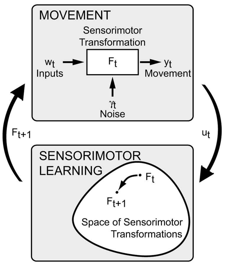
Sensorimotor learning modeled as a dynamic system in the space of sensorimotor transformations. For definitions of variables see Section II.A.
The approach is best illustrated with an example. Consider the case of prism adaptation of visually guided reaching, a well-studied form of sensorimotor learning in which shifted visual feedback drives rapid recalibration of visually guided reaching (von Helmholtz, 1867). Prism adaptation has almost always been studied in a blocked experimental design, with exposure to shifted visual feedback occurring over a block of reaching trials. Adaptation is then quantified by the “after-effect”, the change in the mean reach error across two blocks of no-feedback test reaches, one before and one after the exposure block (Held and Gottlieb, 1958). This experimental approach has had many successes, for example identifying different components of adaptation (Hay and Pick, 1966; Welch et al., 1974) and the experimental factors that influence the quality of adaptation (e.g., Baraduc and Wolpert, 2002; Norris et al., 2001; Redding and Wallace, 1990). However, adaptation is a dynamical process, with behavioral and neural changes in both the behavior and the underlying patterns of neural activity occurring on every trial. Our goal is to describe how the state of the system, which in this case could be modeled as the mean reach error, changes after each trial in response to error feedback (reach errors, perceived visual-proprioceptive misalignment, etc.) on that trial. As we will describe, a comparison of the performance before and after the training block is not sufficient to characterize this process.
Only recently have investigations of sensorimotor learning from a dynamical systems perspective begun to appear (Baddeley et al., 2003; Donchin et al., 2003; Scheidt et al., 2001; Thoroughman and Shadmehr, 2000). While these investigations have all made use of the LDS model class they primarily focused on the application of these methods. A number of important algorithmic and statistical issues that arise when applying these methods remain unaddressed.
Here we outline a general framework for modeling sensorimotor learning with LDS models, discuss the key analytical properties of these models, and address the statistical issues that arise when estimating model parameters from experimental data. We show how LDS can account for performance bias and the decay of learning over time, observed properties of adaptation that have not been included in previous studies. We show that the decay effect can be confounded with the effects of sensory feedback and that it can be difficult to separate these effects statistically. In contrast, the effects of exogenous inputs that are uncorrelated with the state of the sensorimotor transformation are much easier to characterize. We describe a novel resampling-based hypothesis test that can be used to identify the significance of such effects.
The estimation of the LDS model parameters requires an iterative, maximum likelihood, system identification algorithm (Ghahramani and Hinton, 1996; Shumway and Stoffer, 1982), which we present in a slightly modified form. This iterative algorithm is necessary because, as we show, simple linear regression approaches are biased and/or ineffcient. The maximum-likelihood model can be used to quantify characteristics of the dynamics of sensorimotor learning and can make testable predictions for future experiments. Finally, we illustrate this framework with an application to a modern variant of the prism adaptation experiment.
II. A LINEAR DYNAMICAL SYSTEMS MODEL FOR SENSORIMOTOR LEARNING
A. General formulation of the model
Movement control can be described as a transformation of sensory signals into motor outputs. This transformation is generally a continuous-time stochastic process that includes both internal (“efference copy”) and sensory feedback loops. We will use the term “sensorimotor transformation” to refer to the input-output mapping of this entire process, feedback loops and all. This definition is useful in the case of discrete movements and other situations where continuous time can be discretized in a manner that permits a concise description of the feedback processes within each timestep. We assume that at any given movement trial or discrete timestep, indexed by t, the motor output can be quantified by a vector yt. In general, this output might depend on both a vector of inputs wt to the system and the “output noise” γt, the combined effect of sensory, motor, and processing variability. As shown in the upper box of Fig. 1, the sensorimotor transformation can be formalized as a time-varying function of these two variables,
| (1a) |
We next define “sensorimotor learning” as a change in the transformation Ft in response to the sensorimotor experience of previous movements, as shown in the lower box of Fig. 1. We let ut represent the vector of sensorimotor variables at timestep t that drive such learning. This vector might include exogenous inputs rt and, since feedback typically plays a large role in learning, the motor outputs yt. The input ut might have all, some or no components in common with the inputs wt. Generally, learning after timestep t can depend on the complete history of this variable, Ut ≡ {u1,…,ut}. Sensorimotor learning can then be modeled as a discrete-time dynamical system whose state is the current sensorimotor transformation, Ft, and whose state-update equation is the “learning rule” that specifies how F changes over time:
| (1b) |
where the noise term ηt includes sensory feedback noise as well as intrinsic variability in the mechanisms of learning and will be referred to as “learning noise”.
Previous studies that have adopted a dynamical systems approach to studying sensorimotor learning have only taken the output noise into account (Baddeley et al., 2003; Donchin et al., 2003; Thoroughman and Shadmehr, 2000). However, it seems likely that variability exists both in the sensorimotor output and in the process of sensorimotor learning. Attempts to fit empirical data with parametric models of learning that do not account for learning noise may yield incorrect results (see Section IV.D for an example). Aside from these practical concerns, it is also of intrinsic interest to quantify the relative contributions of the output and learning noise to performance variability.
B. The class of LDS models
The model class defined in Eqn. 1 provides a general framework for thinking about sensorimotor learning, but it is too general to be of practical use. Here we outline a series of assumptions that lead us from the general formulation to the specific class of LDS models, which can be a practical yet powerful tool for interpreting sensorimotor learning experiments.
Stationarity: On the time scale that it takes to collect a typical dataset the learning rule L does not explicitly depend on time.
Parameterization: Ft can be written in parametric form with a finite number of parameters, xt ∈ Rm. This is not a serious restriction, as many finite basis functions sets can describe large classes of functions. The parameter vector xt now represents the state of the dynamical system at time t, and Xt is the history of these states. The full model, consisting of the learning rule L and sensorimotor transformation F, is now given by
| (2a) |
| (2b) |
-
Markov Property: The evolution of the system depends only on the current state and inputs, not on the full history:
(3a) (3b) In other words, we assume “online” or “incremental” learning, as opposed to “batch” learning, a standard assumption for models of biological learning.
-
Linear Approximation and Gaussian Noise: The functions F and L can be linearized about some equilibrium values for the states (xe), inputs (ue and we), and outputs (ye):
(4a) (4b) Thus, if the system were initially set-up in equilibrium, the dynamics would be solely driven by random fluctuations about that equilibrium. The linear approximation is not unreasonable for many experimental contexts in which the magnitude of the experimental manipulation, i.e., the inputs, are small, since in these cases the deviations from equilibrium of the state and the output are small.
-
The combined effect of the constant equilibrium terms in Eqn. 4 can be lumped into a single constant “bias” term for each equation:
(5a) (5b) We will show in Section III.B that it is possible to remove the effects of the bias terms bx and by from the LDS. In anticipation of that result, we will drop the bias terms in the following discussion.
With the additional assumption that ηt and γt are zero-mean, Gaussian white noise processes, we arrive at the LDS model class we use below:(6a) (6b) with(6c) In principle, signal-dependent motor noise (Clamann, 1969; Harris and Wolpert, 1998; Matthews, 1996; Todorov and Jordan, 2002) could be incorporated into this model by allowing the output variance R to vary with t. In practice, this would complicate parameter estimation. In the case where the data consists of a set of discrete movements with similar kinematics (e.g. repeated reaches with only modest variation in start and end locations), the modulation of R with t would be negligible. We will restrict our consideration to the case of stationary R.
Among the LDS models defined in Eqn. 6 there are distinct subclasses that are functionally equivalent. The parameters of two equivalent models are related to each other by a similarity transformation of the states xt
| (7) |
where P is an invertible matrix. This equivalence exists because the state cannot be directly observed, but must be inferred from the outputs yt. An LDS from one subclass of equivalent models cannot be transformed into an LDS of another subclass via Eqn. 7. In particular, a similarity transformation of an LDS with A = I always yields another LDS with A = I since
| (8) |
Therefore, it is restrictive to assume that A = I, i.e. that there is no “decay” of input-driven state changes over time.
The equivalence under similarity transformation can be useful if one wishes to place certain constraints on the LDS parameters. For instance, if one wishes to identify state components that evolve independently in the absence of sensory inputs, then the matrix A has to be diagonal. In many cases1 this constraint can be met by performing unconstrained parameter estimation and then transforming the parameters with P = [υ1…υn]−1, where vi are the eigenvectors of the estimate of A. The transformed matrix A′= PAP−1 is a diagonal matrix composed of the eigenvalues of A. As another example, the relationship between the state and the output might be known, i.e. C = C0. If both C0 and the estimated value of C are invertible, this constraint is achieved by transforming the estimated LDS with .
C. Feedback in LDS models
In the LDS model of Eqn. 6, learning is driven by an input vector ut. In an experimental setting, the exact nature of this signal will depend on the details of the task and is likely to be unknown. In general, it can include sensory feedback of the previous movement as well as exogenous sensory inputs. When we consider the problem of parameter estimation in Section IV, we will show that the parameters corresponding to these two components of the input have different statistical properties. Therefore, we will explicitly write the input vector as , where the vector rt contains the exogenous input signals. We will similarly partition the input parameter, B = [G H]. This yields the form of the LDS model that will be used in the subsequent discussion:
| (9a) |
| (9b) |
| (9c) |
The decomposition of ut specified above is not overly restrictive, since any feedback signal can be divided into a component that is uncorrelated with the output (rt above) and a component that is a linear transformation of the output. Furthermore, Eqn. 9 can capture a variety of common feedback models. To illustrate this point, we consider three forms of “error corrective” learning.
In the first case, learning is driven by the previous performance error, , where is the target output. As an example, could be a visual reach target and ut could be the visually perceived reach error. If we let and G = H, then Eqn. 9a acts as a feedback controller designed to reduce performance error.
As a second form of error corrective learning, consider the case where learning is driven by the unexpected motor output, ut = yt – y^t, where y^t = Cxt + Dwt is the predicted motor output. This learning rule would be used if the goal of the learner were to accurately predict the output of the system given the inputs ut and wt, i.e. to learn a “forward model” of the physical plant y^(ut, wt, xt) (Jordan and Rumelhart, 1992). Writing this learning rule in the LDS form of Eqn. 6a, we obtain
Thus, this scheme can be expressed in the form of Eqn. 9a, with rt = wt and parameters A′, G′, and H′.
Finally, learning could be driven by the predicted performance error, (e.g., Donchin et al., 2003; Jordan and Rumelhart, 1992). This scheme would be useful if the learner already had access to an accurate forward model. Using the predicted performance to estimate movement error would eliminate the effects that motor variability and feedback sensor noise have on learning. Also, in the context of continuous time systems, learning from the predicted performance error minimizes the effects of delays in the feedback loop. Putting this learning rule into the form of Eqn. 6a, we obtain
Again, this scheme is consistent with Eqn. 9a, with the inputs rt and parameters A′ and G′ and H = 0.
D. Example Applications
LDS models can be applied to a wide range of sensorimotor learning tasks, but there are some restrictions. The true dynamics of learning must be consistent with the assumptions underlying the LDS framework, as discussed in Section II.B. Most notably, both the learning dynamics and motor output have to be approximately linear within the range of states and inputs experienced. In addition, LDS models can only be fit to experimental data if the inputs ut and outputs yt are well-defined and can be measured by the experimenter. Identifying inputs amounts to defining the error signals that could potentially drive learning. While the true inputs will typically not be known a priori, it is often the case that several candidate input signals are available. Hypothesis testing can then be used to determine which signals contribute significantly to the dynamics of learning, as discussed below in Section IV.B. The outputs yt must be causally related to the state of the sensorimotor system, since it functions as a noisy read-out of the state. Several illustrative examples are described here.
Consider first the case where t represents discrete movements. Two example tasks would be goal directed reaching and hammering. A reasonable choice of state variable for these tasks would be the average positional error at the end of the movement. In this case, yt would be the error on each trial. In the hammering task, one might also include task-relevant dynamic information such as the magnitude and direction of the impact force. In some circumstances, these endpoint-specific variables might be affected too much by online feedback to serve as a readout of the sensorimotor state. In such a case, one may choose to focus on variables from earlier in the movement (e.g., Donchin et al., 2003; Thoroughman and Shadmehr, 2000). Indeed, a more complete description of the sensorimotor state might be obtained by augmenting the output vector by multiple kinematic or dynamic parameters of the movement and similarly increasing the dimensionality of the state. In the reaching task, for example, yt could contain the position and velocity at several time-points during the reach. Similarly, the output for the hammering task might contain snapshots of the kinematics of the hammer or the forces exerted on the hammer by the hand. If learning is thought to occur independently in different components of the movement, then state and output variables for each component should be handled by separate LDS models in order to reduce the overall model complexity.
Next, consider the example of gain adaptation in the vestibular ocular reflex (VOR). The VOR stabilizes gaze direction during head rotation. The state of the VOR can be characterized by its “gain”, the ratio of the angular speed of the eye response over the speed of the rotation stimulus. When magnifying or minimizing lenses are used to alter the relationship between head rotation and visual motion, VOR gain adaptation is observed (Miles and Fuller, 1974). An LDS could be used to model this form of sensorimotor learning with the VOR gain as the state of the system. If the output is chosen to be the empirical ratio of eye and head velocity, then a linear equation relating output to state is reasonable. The input to the LDS could be the speed of visual motion or the ratio of that speed to the speed of head rotation. On average, such input would be zero if the VOR had perfect gain. A more elaborate model could include separate input, state, and output variables for movement about the horizontal and vertical axes. The dynamics of VOR adaptation could be modeled across discrete trials, consisting, for example, of several cycles of sinusoidal head rotations about some axis. The variables yt and ut could then be time averages over trial t of the respective variables. On the other hand, VOR gain adaptation is more accurately described as a continuous learning process. This view can also be incorporated into the LDS framework. Time is discretized into timesteps indexed by t, and the variables yt and ut represent averages over each timestep.
In the examples described so far, the input and output error signals are explicitly defined with respect to some task-relevant goal. It is important to note, however, that the movement goal need not be explicitly specified or directly measurable. There are many examples where sensorimotor learning occurs without an explicit task goal: when auditory feedback of vowel production is pitch-shifted, subjects alter their speech output to compensate for the shift (Houde and Jordan, 1998); when reaching movements are performed in a rotating room, subjects adapt to the Coriolis forces to produce nearly straight arm trajectories even without visual feedback (Lackner and Dizio, 1994); when the visually perceived curvature of reach trajectories are artificially shifted, subjects adapt their true arm trajectories to compensate for the apparent curvature (Flanagan and Rao, 1995; Wolpert et al., 1995). What is common to these examples is an apparent implicit movement goal that subjects are trying to achieve. The LDS approach can still be applied in this common experimental scenario. In this case, a measure of the trial-by-trial deviation from a baseline (pre-exposure) movement can serve as a measure of the state of sensorimotor adaptation or as an error feedback signal. This approach has been applied successfully in the study of reach adaptation to force perturbations (Donchin et al., 2003; Thoroughman and Shadmehr, 2000).
III. CHARACTERISTICS OF LDS MODELS
We now describe how the LDS parameters relate to two important characteristics of sensorimotor learning, the steady state behavior of the learner and the effects of performance “bias”.
A. Dynamics vs. steady state
Most experiments of sensorimotor learning have focused on the “after-effect” of learning, measured as the change in motor output following a block of repeated exposure trials. The LDS can be used to model such blocked exposure designs. An LDS with constant exogenous inputs (rt = r, wt = w) will, after many trials, approach a steady state in which the state and output are constant except for fluctuations due to noise. The after-effect is essentially the expected value of the steady state output,
| (10) |
An expression for the steady state x∞= limt→∞ E (xt) is obtained by taking the expectation value and then the limit of Eqn. 9a, yielding
| (11) |
Combining Eqns. 10 and 11, the steady state is given by the solution of
| (12) |
A unique solution to Eqn. 12 exists only if A + HC − I is invertible. One sufficient condition for this is asymptotic stability of the system, which means that the state converges to zero as t → ∞ in the absence of any inputs or noise. This follows from the fact that a system is asymptotically stable if and only if all of the eigenvalues of A + HC have magnitude less than unity (Kailath, 1980). When a unique solution exists, it is given by
| (13) |
and the steady-state output is
| (14) |
This last expression can be broken down into the effective “gains” for the inputs r and w, i.e. the coefficients C(A + HC − I)−1G and C(A+HC−I)−1HD+D, respectively. While these two gains can be estimated from the steady-state output in a blocked-exposure experiment, they are insufficient to determine the full system dynamics. In fact, none of the parameters of the LDS model in Eqn. 9 can be directly estimated from these two gains.
The difference between studying the dynamics and the steady state is best illustrated with examples. We consider the performance of two specific LDS models. For simplicity, we place several constraints on the LDS: C = I, meaning the state x represents the mean motor output; D = 0, meaning the exogenous input has no direct effect on the current movement; and G and H are invertible, meaning that no dimensions of the input r or feedback yt are ignored during learning. In the first example, we consider the case where A = I. This is a system with no intrinsic “decay” of the learned state. From Eqn. 14, we see that the steady-state output in this case converges to the value
| (15) |
If this is a simple error corrective learning algorithm as in the first example of Section II.C, then G = H and the output converges to a completely adaptive response in the steady-state, y∞ = −r. In such a case, the steady-state output is independent of the value of H, and so experiments that measure only the steady-state performance will miss the dynamical effects due to the structure of H. Such effects are illustrated in Fig. 2, which shows the simulated evolution of the state of the system when the learning rate along the x-direction (H11) is 40% smaller than in the y-direction (H22). Such spatial anisotropies in the dynamics of learning provide important clues about the underlying mechanisms of learning. For example, anisotropies could be used to identify differences in the learning and control of specific spatial components of movement (Favilla et al., 1989; Krakauer et al., 2000; Pine et al., 1996).
FIG. 2.
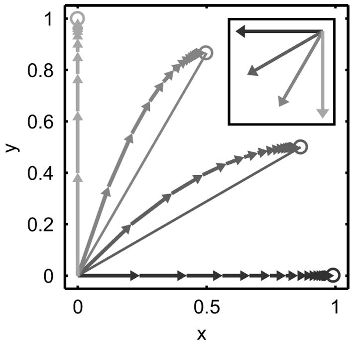
Illustration of the difference between trial-by-trial state of adaptation (connected arrows) and steady-state of adaptation (open circles) in a simple simulation of error corrective learning. The data were simulated with no noise and with diagonal matrices G = H. The learning rate in the x-direction, H11, was 40% smaller than in the y-direction, H22. Four different input vectors were used, as shown in the inset in the corresponding shade of gray.
In the second example, we consider a learning rule that does not achieve complete adaptation, a more typical outcome in experimental settings. Unlike in the last example, we assume that the system is isotropic, i.e. A = aI, G = −gI, and H = −hI, where a, g, and h are positive scalars. In this case the steady-state output is
| (16) |
A system with a = 1 and g = h will exhibit complete adaptation, i.e., y∞ = −r. However, incomplete adaptation, |y∞| < |r|, could be due either to state decay (a < 1) or to a greater weighting of the feedback signal compared to the exogenous shift (h > g). Measurements of the steady state are not sufficient to distinguish between these two qualitatively different scenarios. These examples illustrate that knowing the steady-state output does not fully constrain the important features of the underlying mechanisms of adaptation.
B. Modeling sensorimotor bias
The presence of systematic errors in human motor performance is well documented (e.g., Gordon et al., 1994; Soechting and Flanders, 1989; Weber and Daroff, 1971). Such “sensorimotor biases” could arise from a combination of sensory, motor, and processing errors. While bias has not been considered in previous studies using LDS models, failing to account for it can lead to poor estimates of model parameters. Here, we show how sensorimotor bias can be incorporated into the LDS model and how the effects of bias on parameter estimation can be avoided.
It might seem that the simplest way to account for sensorimotor bias would be to add a bias vector by to the output equation (Eqn. 9):
| (17a) |
| (17b) |
However, in a stable feedback system, feedback-dependent learning will effectively adapt away the bias. This can be seen by examining the steady state of Eqn. 17,
Considering the case where A = I, and C and H are invertible, the steady state compensates for the bias, x∞ = −C−1(H−1Gr + Dw + by), and so the bias term vanishes entirely from the asymptotic output: y∞ = −H−1Gr.
The simplest way to capture a stationary sensorimotor bias in an LDS model is to incorporate it into the learning equation. For reasons that will become clear below, we add a bias term −Hbx,
| (18a) |
| (18b) |
Now the bias carries through to the sensorimotor output:
Again assuming that A = I, and C and H are invertible, the stationary output becomes y∞ = −H−1Gr + bx, which is the unbiased steady-state output plus the bias vector bx.
As described in Section II, the sensorimotor biases defined above are closely related to the equilibrium terms xe, ye, etc., in Eqn. 4. If Eqn. 18 were fit to experimental data, the bias term bx would capture the combined effects of all the equilibrium terms in Eqn. 4a. Similarly, a bias term by in the output equation would account for the equilibrium terms in Eqn. 4b. However, adding these bias parameters to the model would increase the model complexity with little benefit, as it would be very difficult to interpret these composite terms. Here we show how bias can be removed from the data so that these model parameters can be safely ignored.
With T being the total number of trials or timesteps, let and ū, w̄, and ȳ defined accordingly. Averaging Eqn. 5 over t, we get
With the approximations and , which are quite good for large T, we get
Subtracting these equations from Eqn. 5 leads to
| (19) |
| (20) |
Therefore, the mean-subtracted values of the empirical input and output variables obey the same dynamics as the raw data, but without the bias terms. This justifies using Eqn. 6 to model experimental data, as long as the inputs and outputs are understood to be the mean-subtracted values.
IV. PARAMETER ESTIMATION
Ultimately, LDS models of sensorimotor learning are only useful if they can be fit to experimental data. The process of selecting the LDS model that best accounts for a sequence of inputs and outputs is called “system identification” (Ljung, 1999). Here we take a maximum-likelihood approach to system identification. Given a sequence (or sequences) of input and output data, we wish to determine the model parameters for Eqn. 9 for which the dataset has the highest likelihood, i.e., we want the maximum likelihood estimates (MLE) of the model parameters. Since no analytical solution exists in this case, we employ the expectation-maximization (EM) algorithm to calculate the MLE numerically (Dempster et al., 1977). A review of the EM algorithm for LDS (Ghahramani and Hinton, 1996; Shumway and Stoffer, 1982) is presented in the Appendix, with one algorithmic refinement. A Matlab implementation of this EM algorithm is freely available online at http://keck.ucsf.edu/~sabes/software/. Here we discuss several issues that commonly arise when trying to fit LDS models that include sensory feedback.
A. Correlation between parameter estimates
Generally, identification of a system operating under closed-loop (i.e. where the output is fed back to the learning rule) is more difficult than if the same system were operating in open loop (no feedback). This is partly because the closed loop makes the system less sensitive to external input (Ljung, 1999). In addition, and perhaps more importantly for our application, since the output directly affects the state, these two quantities tend to be correlated. This makes it difficult to distinguish their effects on learning, i.e. to fit the parameters A and H.
To determine the conditions that give rise to this difficulty consider two hypothetical LDS models
| (21) |
| (22) |
which are related to each other by A′ = A – δC and H′ = H + δ. These models differ in how much the current state affects the subsequent state directly (A) or through output feedback (H), and the difference is controlled by d. However, the total effect of the current state is the same in both models, i.e., A + HC = A′+ H′C. Distinguishing these two models is thus equivalent to separating the effects of the current state and the feedback on learning. To determine when this distinction is possible we rewrite the second LDS in terms of A and H:
| (23) |
where the last step uses Eqn. 9b. Comparing Eqns. 21 and 23, we see that the two models are easily distinguished if the contribution of the δDwt term is large. However, in many experimental settings the exogenous input has little affect on the ongoing motor output (e.g., in the terminal feedback paradigm described in Section V), implying that Dwt is negligible. In this case, the main difference between these two models is the noise term δγt, and the ability to distinguish between the models depends on the relative magnitudes of the variances of the output and learning noise terms, R = Var(γt) and Q = Var(ηt). For |R| ≫ |Q|, separation will be relatively easy. In other cases, the signal due to δγt may be lost in the learning noise.
We next fit a one-dimensional LDS to simulated data in order to confirm the correlation between the estimates for A and H and to investigate other potential correlations among parameter estimates. In these simulations, the inputs rt and the learning noise ηt were both zero-mean, Gaussian white noise processes. Both variables had unity variance, determining the scale for the other parameters values, which are listed in Fig. 3. Three different values for and two dataset lengths T were used. Note that the input affects learning via the product Gr, and so the standard deviation of this product quantifies the input effect. Here and below we use |Gr| to refer to this standard deviation. For each pair of values for and T we simulated 1000 datasets and estimated the LDS parameters with the EM algorithm. We then calculated the correlations between the various parameter estimates across simulated datasets (Fig. 3). With sufficiently large datasets the MLE are consistent and exhibit little variability (Fig. 3, bottom row). If the datasets are relatively small, two different effects can be seen, depending on the relative magnitudes of R and Q. As predicted above, when R < Q there is large variability in the estimates  and Ĥ and they are negatively correlated (Fig. 3, top-left panel). In separate simulations (data not shown), we confirmed that this correlation disappears when there are substantial feedthrough inputs, i.e., when |Dw| is large. In contrast, when the output noise has large variance, R > Q, the estimate R̂ covaries with the other model parameters (Fig. 3, top-right panel). This effect has an intuitive explanation: when the estimated output variance is larger than the true value, even structured variability in the output is counted as noise. In other words, a large R̂ masks the effects of the other parameters, which are thus estimated to be closer to zero.
FIG. 3.
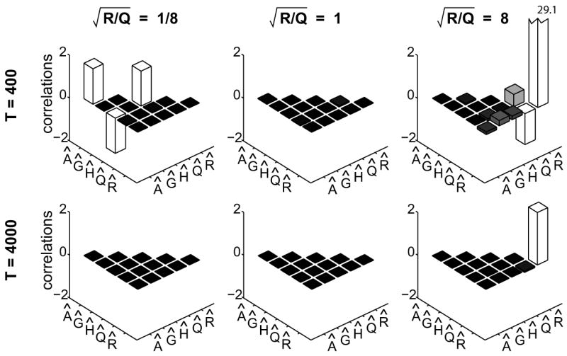
Correlations between LDS parameter estimates across 1000 simulated datasets. Each panel corresponds to a particular value for T and . Simulations used an LDS with parameters A = 0.8, |Gr| = 0.5, H = −0.2, C = 1, D = 0, Q = 1, and zero-mean, white noise inputs rt with unit variance.
Next, we isolate and quantify in more detail the correlation between the estimates  and Ĥ. We computed the MLE for simulated data under two different constraint conditions. In the first case, only Ĥ was fit to the data, while all other parameters were fixed at their true values (H unknown, A known). In the second case, the sum A + HC and all parameters other than A and H were fixed to their true values (A and H unknown, A + HC known). In this case,  and Ĥ were constrained to be A − δC and H + δ, respectively, and the value of δ was fit to the data. This condition tests directly whether the maximum likelihood approach can distinguish the effects of the current state and the feedback on learning. Under both of these conditions there is only a single free parameter, and so a simple line search algorithm was used to find the MLE of the parameter from simulated data.
Data were simulated with the same parameters as in Fig. 3 while three quantities were varied: , |Gr|, and T (see Fig. 4). For a given set of parameter values we simulated 1000 datasets and found the MLE Ĥ for each. The 95%-confidence interval (CI) for Ĥ was computed as the symmetric interval around the true H containing 95% of the fit values Ĥ.
FIG. 4.
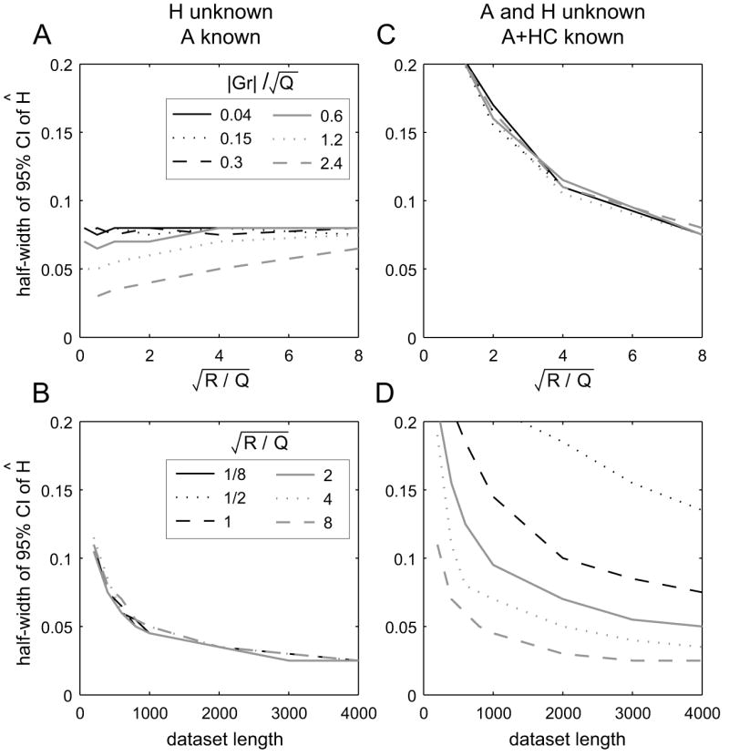
Uncertainty in the feedback parameter Ĥ in two different constraint conditions. All data were simulated with parameters A = 0.8, H = −0.2, C = 1, D = 0. Q sets the scale. A: Variability of Ĥ as a function of the output noise magnitude, when all other parameters, in particular A, are known (T = 400 trials). Lines correspond to different values of the magnitude of the exogenous input signal. B: Variability of Ĥ as a function of dataset length, T, for |Gr| = 0 (no exogenous input). Lines correspond to different levels of output noise. C and D: Variability of Ĥ when both H and A are unknown, but A + HC, as well as all other parameters, are known; otherwise as in A and B, respectively.
The results for the first constraint case (H unknown) are shown on the left side of Fig. 4. Uncertainty in Ĥ is largely invariant to the magnitude of the output noise or the exogenous input signal, |Gr|, although there is a small interaction between the two at high input levels. For later comparison, we note that with T = 1000, we obtain a 95%-CI of ±0.05.
The results are very different when A + HC is fixed but A and H are unknown (right side of Fig. 4). While the uncertainty in Ĥ is independent of the input magnitude, it is highly dependent on the magnitude of the output noise. As predicted, when R is small relative to Q, there is much greater uncertainty in Ĥ compared to the first constraint condition. For example, if (comparable to the empirical results shown in Fig. 8C below) several thousands of trials would needed to reach a 95%-CI of ±0.05. In order to match the precision of Ĥ obtained in the first constraint condition with T = 1000, is needed.
FIG. 8.
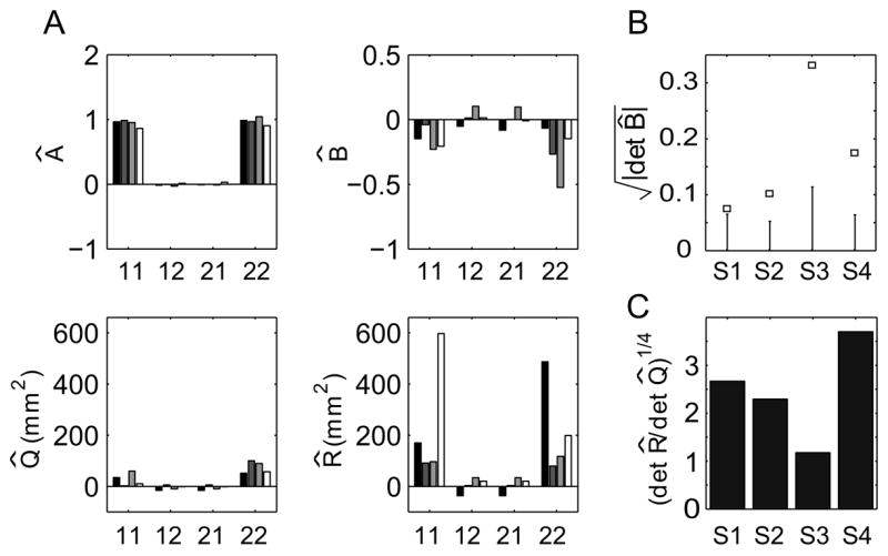
A: Estimated LDS parameters  , B̂, Q̂, and R̂ for four subjects. Labels on the x-axis indicate the components of each matrix. Each bar shading corresponds to a different subject (S1–S4). B: Results of permutation test for the input parameter B for each subject. The square marks and the errorbars show the 95% confidence interval for that value given H0 : det B = 0, generated from 1000 permuted datasets. C: Estimate of ratio of output to learning noise standard deviation.
B. Hypothesis testing
One important goal in studying sensorimotor learning is to identify which sensory signal, or signals, drive learning. Consider the case of a k-dimensional vector of potential input signals, rt. We wish to determine whether the ith component of this input has a significant effect on the evolution of the state, i.e. whether Gi, the ith column of G, is significantly different from zero. Specifically, we would like to test the hypothesis H1: Gi ≠ 0 against the null hypothesis H0: Gi = 0. Given the framework of maximum likelihood estimation, we could use a generic likelihood ratio test in order to assess the significance of the parameters Gi (Draper and Smith, 1998). However, the likelihood ratio test is only valid in the limit of large datasets. Given the complexity of these models, that limit may not be achieved in typical experimental settings.
Instead, we propose the use of a permutation test, a simple class of non-parametric, resampling-based hypothesis tests (Good, 2000). Consider again the null hypothesis H0: Gi = 0, which implies that , the ith component of the exogenous input rt, does not influence the evolution system. If H0 were true, then randomly permuting the values of across t should not affect the quality of the fit — in any case we expect Gi to be near zero. This suggests the following permutation test. We randomly permute the ith component of the exogenous input, determine the MLE parameters of the LDS model from the permuted data, and compute a statistic representing the goodness-of-fit of the MLE, in our case the log likelihood of the permuted data given the MLE, Lperm. This process is repeated many times. The null hypothesis is then rejected at the (1 − α)-level if the fraction of Lperm that exceed the value of L computed from the original dataset is below α. Alternatively, the magnitude of Gi itself could be used as the test statistic, since Gi is expected to be near zero for the permuted datasets.
To evaluate the usefulness of the permutation test outlined above, we performed a power analysis on datasets simulated from the one-dimensional LDS described in Fig. 5. For each combination of parameters we simulated 100 datasets. For each of these datasets, we determined the significance of the scalar G using the permutation test described above with k = i = 1, α = 0.05, and 500 permutations of rt. The fraction of datasets for which the null hypothesis was (correctly) rejected represents the power of the permutation test for those parameter values.
FIG. 5.
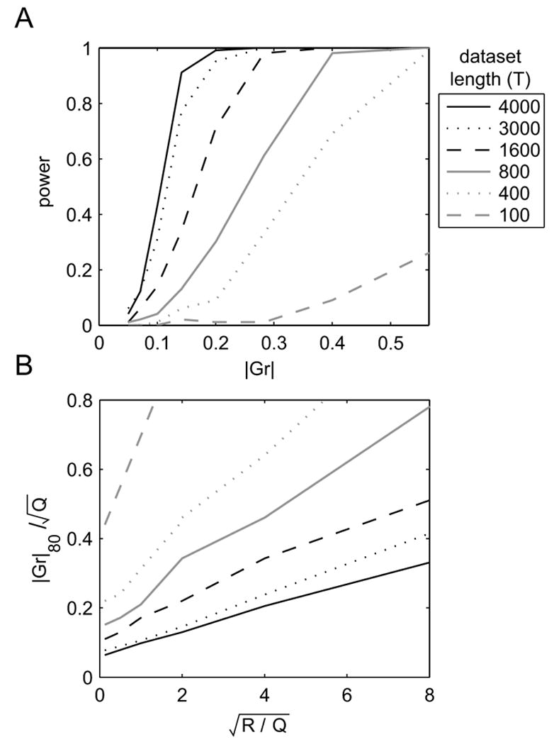
Power analysis of the permutation test for the significance of G. Simulation parameters: A = 0.8, H = −0.2, C = 1, and D = 0. Q sets the scale. A: Statistical power when . B: Input magnitude required to achieve 80% power, as a ratio of . In both panels, α = 0.05 and line type indicates the dataset length T.
The top panel of Fig. 5 shows the power as a function of the input magnitude and trial length T, given . The lower panel shows the magnitude of the input required to obtain a power of 80%, as a function of and T. Plots such as these should be used during experimental design. However, since neither G nor the output and learning noise magnitudes are typically known, heuristic values must be used. With and , approximately 1600 trials are needed to obtain 80% power. Note, however, that the exogenous input signal is often under experimental control. In this case, the same power could be achieved with about 400 trials if the magnitude of that signal were doubled. In general, increasing the amplitude of the input signal will allow the experimenter to achieve any desired statistical power for this test. Practically, however, the size of a perturbative input signal is usually limited by several factors, including physical constraints or a requirement that subjects remain unaware of the manipulation. Therefore, large numbers of trials may often be required to achieve sufficient power.
C. Combining multiple datasets
A practical approach to collecting larger datasets is to perform repeated experiments, either during multiple sessions with a single subject or with multiple subjects. In either case, accurate model fitting requires that the learning rule is stationary (i.e., constant LDS parameters) across sessions or subjects. There are two possible approaches to combining N datasets of length T. First, the data from different sessions can be concatenated to form a “super dataset” of length NT. The system identification procedure outlined in the Appendix can be directly applied to the super dataset with the caveat that the initial state xt=1 has to be reset at the beginning of each dataset.
A second approach can be taken when nominally identical experiments are repeated across sessions, i.e. when the input sequences rt and wt are the same in each session. In this approach the inputs and outputs are averaged across sessions, yielding a single “average dataset” with inputs r̃t and w̃t, and outputs ỹt. The dynamics underlying this average dataset are obtained by averaging the learning and output equations for each t (Eqn. 9) across datasets:
| (24a) |
| (24b) |
Note that the only difference between this model and that describing the individual datasets is that the noise variances have been scaled: Var(η̃t) = Q/N and Var(γ̃t) = R/N. Therefore, the EM algorithm (see Appendix) can be directly applied to average datasets as well.
Since both approaches to combining multiple datasets are valid, we ran simulated experiments to determine which approach produces better parameter estimates, i.e., tighter confidence intervals. Simulations were performed with the model described in Fig. 6, varying R and Q while maintaining a fixed ratio .
FIG. 6.
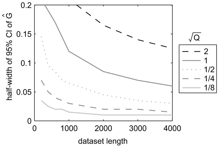
95%-confidence intervals for the MLE of the input parameter G, computed from 1000 simulated datasets. All simulations were run with and Gaussian white noise inputs with zero-mean and unit variance. A = 0.8, G = −0.3, H = −0.2, C = 1, and D = 0.
The preferred approach for combining datasets depends on which parameter one is trying to estimate. CIs for the exogenous input parameter Ĝ are shown in Fig. 6. Variability depends strongly on the number of trials but even more so on the noise variances. For example, with 200 trials, R = 1, and Q = 1/2, the 95%-CI is ±0.145. Multiplying the number of trials by 4 results in a 41% improvement in CI, yet dividing the noise variances by 4 yields a 76% improvement. Therefore, for estimating G it is best to average the datasets. It should be noted, however, that the advantage is somewhat weaker for larger input variances (Fig. 6 was generated with unit input variance; other data not shown). By contrast, the variability of the MLE for H only mildly depends on the noise variances (data not shown), if at all. Therefore, increasing the dataset length by concatenation produces better estimates for H than decreasing the noise variances by averaging.
D. Linear regression
As noted above, there is no analytic solution for the maximum likelihood estimators of the LDS parameters, so the EM algorithm is used (Ghahramani and Hinton, 1996; Shumway and Stoffer, 1982). While EM has many attractive properties (Dempster et al., 1977), it is a computationally expensive, iterative algorithm and it can get caught in local minima. The computation time becomes particularly problematic when system identification is used in conjunction with resampling schemes for statistical analyses such as bootstrapping (Efron and Tibshirani, 1993) or the permutation tests described above. It is therefore tempting to circumvent the inefficiencies of the EM algorithm by converting the problem into one that can be solved analytically. Specifically, there have been attempts to fit a subclass of LDS models using linear regression (e.g., Donchin et al., 2003). It is, in fact, possible to find a regression equation for the input parameters G, H, and D if we assume that A = I, a fairly strict constraint implying no state decay. There are then two possible approaches to transforming system identification into a linear regression problem. As we describe here, however, both approaches can lead to inefficient, or worse, inconsistent estimates.
First we consider the “subtraction approach”. If A = I, the following expression for the trial-by-trial change in output can be derived from the LDS in Eqn. 6 (i.e., the form without explicit feedback),
| (25) |
This equation suggests that the trial-by-trial changes in yt can be regressed on inputs ut and wt in order to determine the parameters CB and D. Obtaining an estimate of B requires knowing C, however that is not a significant constraint due to the existence of the similarity classes described in Eqn. 7. One complication with this approach is that the noise terms in Eqn. 25, γt+1 − γt + Cηt are correlated across trials. Such colored noise can be accommodated in linear regression (Draper and Smith, 1998), however the ratio of R and Q would have to be known in order to construct an appropriate covariance matrix for the noise. A more serious problem with the regression model in Eqn. 25 arises in feedback systems, in which But = Grt + Hyt. In this case, the RHS of equation Eqn. 25 contains the same term, yt, as the LHS. This correlation between the dependent variables yt and the independent variables yt+1 – yt leads to a biased estimates for H. As an example, consider a sequence yt that is generated by a pure, white-noise process with no feedback dynamics. If the regression model of equation Eqn. 25 were applied to this sequence, with C = 1 and no exogenous inputs, the expected value of the regression parameter would be Ĥ = −1, compared to the true value H = 0. Application of the regression model in Eqn. 25 to simulated data confirms this pattern of bias in Ĥ (Fig. 7, black line). In the general multivariate case, Ĥ will be biased towards −I as long as the output noise is large compared to the learning noise.
FIG. 7.
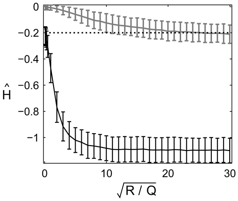
Bias in Ĥ using two different linear regression fits of simulated data. The datasets were simulated with no exogenous inputs and the LDS model parameters A = 1, G = 0, H = −0.2, C = 1, and D = 0. Q sets the scale. The lower (black) data points represent the average Ĥ over 1000 simulated datasets using the subtraction approach. The upper (gray) data points are for the summation approach. The true value of H is shown as the dotted line. Error-bars represent standard deviations.
The bias described above arises from the fact that the term yt occurs on both sides of the regression equation. This problem can be circumvented by deriving a simple expression for the output as a linear function of the initial state and all inputs up to, but not including, the current timestep:
| (26) |
This expression suggests the “summation approach” to system identification by linear regression. The set of Eqns. 26 for each t can be combined into the standard matrix regression equation Y = Xβ+noise:
| (27) |
For a given value of C, regression would produce estimates for x1, G, H, and D. One pitfall with this approach is that the variance of the noise terms grows linearly with the trial count t:
| (28) |
This problem is negligible if |Q| ≪ |R|. Otherwise, as the trial count increases the accumulated learning noise will dominate all other correlations and the estimated parameter values will approach zero. This effect can be seen for our simulated datasets in Fig. 7, gray line. Of course, this problem could be addressed by modeling the full covariance matrix of the noise terms and including them in the regression (Eqn. 28 gives the diagonal terms of the matrix). However, this requires knowing Q and R in advance. Also, the linear growth in variance means that later terms will be heavily discounted, forfeiting the benefit of large datasets.
V. EXAMPLE: REACHING WITH SHIFTED VISUAL FEEDBACK
Here we present an application of the LDS framework using a well-studied form of feedback error learning: reach adaptation due to shifted visual feedback. In this experiment, subjects made reaching movements in a virtual environment with artificially shifted visual feedback of the hand. The goal is to determine whether a dynamically changing feedback shift drives reach adaptation and, if so, what the dynamics of learning are.
Subjects were seated with their unseen right arm resting on a table. At the beginning of each trial, the index fingertip was positioned at a fixed start location, a virtual visual target was displayed at location gt, and after a short delay an audible go signal instructed subjects to reach to the visual target. The movement began with no visual feedback, but just before the end of the movement (determined online from fingertip velocity) a white disk indicating the fingertip position appeared (“terminal feedback”). The feedback disk tracked the location of the fingertip, offset from the finger by a vector rt. The fingertip position at the end of the movement is represented by ft.
Each subject performed 200 reach trials. The sequence of visual shifts rt was a random walk in 2-dimensional space. The two components of each step, rt+1 − rt, were drawn independently from a zero-mean normal distribution with a standard deviation of 10mm and with the step magnitude limited to 20mm. In addition, each component of rt was limited to the ±60mm range, with reflective boundaries. These limitations were chosen to ensure that subjects did not become aware of the visual shift.
In order to model this learning process with an LDS, we need to define its inputs and outputs. Reach adaptation is traditionally quantified with the “after-effect”, i.e. the reach error yt = ft – gt measured in a no-feedback test reach (Held and Gottlieb, 1958). In our case, the terminal feedback appeared sufficiently late to preclude feedback-driven movement corrections. Therefore, the error on each movement, yt, is a trial-by-trial measure of the state of adaptation. We will also define the state of the system xt to be the mean reach error at a given trial, i.e., the average yt that would be measured across repeated reaches if learning were frozen at trial t. This definition is consistent with the output equation of the LDS model, Eqn. 9b, if two constraints are placed on the LDS: D = 0 and C = I. The first constraint is valid because of the late onset of the visual feedback. The second constraint resolves the ambiguity of the remaining LDS parameters, as discussed in Section II.B.
We will also assume that the input to the LDS is the visually perceived error, ut = yt + rt. Thus, we are modeling reach adaptation as error corrective learning, with a target output (see Section II.C). Note that with this input variable, But = Hyt + Grt if B = H = G. Using the EM algorithm, the sequence of visually perceived errors (inputs) and reach errors (outputs) from each subject were used to estimate the LDS parameters A, B, Q, and R. The parameter fits from four subjects’ data are shown in Fig. 8A. The decay parameter  is nearly diagonal for all subjects, implying that the two components of the state do not mix and thus evolve independently. Also, the diagonal terms of  are close to 1, which means there is little decay of the adaptive state from one trial to the next.
The individual components of the input parameter B̂ are considerably more variable across subjects. A useful quantity to consider is the square root of the determinant of the estimated input matrix, , which is the geometric mean of the magnitudes of the eigenvalues of B̂. This value, shown in Fig. 8B, is a scalar measure of the incremental state correction due to the visually perceived error on each trial. To determine whether these responses are statistically significant, we performed the permutation test described in Section IV.B on the value of . The null hypothesis was H0 : det B = 0. 2 Figure 8B shows that H0 can be rejected with 95% confidence for all four subjects, and so we conclude that the visually perceived error significantly contributes to the dynamics of reach adaptation.
As discussed in Section IV, the statistical properties of the MLE parameters depend to a large degree on the ratio of the learning and output noise terms. In the present example, the covariance matrices are two-dimensional, and so we quantify the magnitude of the noise terms by the square-root of the their determinants, and , respectively. The ratio of standard deviations is thus (det R̂/det Q̂)1/4. The experimental value of this ratio ranges from 1.2 to 3.7 with a mean of 2.5 (Fig. 8C). These novel findings suggest that learning noise might contribute almost as much to behavioral variability as motor performance noise.
The results presented in Fig. 8 depend on the assumption that the visually perceived error ut drives learning. This guess was based on the fact that ut is visually accessible to the subject and is a direct measure of the subject’s visually perceived task performance. However, several alternatives inputs exist, even if we restrict consideration to the variables already discussed. Note again that the input term But can be expanded to Hyt + Grt. The hypothesis that the visually perceived error drives learning is thus equivalent to the claim that H = G. However the true reach error yt and the visual shift rt could effect learning independently. These variables are not accessible from visual feedback alone, but they could be estimated from comparisons of visual and proprioceptive signals or the predictions of internal forward models. While these estimates might be noisier than those derived directly from vision, this sensory variability is included in the learning noise term, as discussed in Section II.A.
Note that an incorrect choice of input variable ut means that the LDS model cannot capture the true learning dynamics, and so the resulting estimate of learning noise should be high. Indeed, one explanation for the large Q in the model fits above is that an important input signal was missing from the model. The LDS framework itself can be used to address such issues. In this case, we can test the alternative H ≠ G against the null hypothesis H = G by asking whether a significantly better fit is obtained with two inputs, [ut, rt], compared to the single input ut. The permutation test, with permuted rt, would be used. We showed in Section IV.A, however, that such comparisons require more than the 200 trials per subject collected here.
VI. DISCUSSION
Quantitative models, even very simple ones, can be extremely powerful tools for studying behavior. They are often used to clarify difficult concepts, quantitatively test intuitive ideas, and rapidly test alternative hypothesis with “virtual experiments”. However, successful application of such models depends on understanding the properties of the model class being used. The class of LDS models is an increasingly popular tool for studying study sensorimotor learning. We have therefore studied the properties of this model class and identified the key issues that arise in their application.
We explored the steady-state behavior of LDS models and related that behavior to the traditional measures of learning in blocked-exposure experimental designs. These results demonstrate why the dynamical systems approach provides a clearer picture of the mechanisms of sensorimotor learning.
We described the EM-algorithm for system identification and discussed some of the details and difficulties involved in estimating model parameters from empirical data. Most importantly, in closed-loop systems it is difficult to separate the effects of state decay (A) and feedback (H) on the dynamics of learning. Note that this limitation is an example of a more general difficulty with all linear models. If any two variables in either the learning or output equations are correlated, then it will be difficult to independently estimate the coefficients of those variables. For example, if the exogenous learning signal rt and feedthrough input wt are correlated in a feedback system, then it is difficult to distinguish the exogenous and feedback learning parameters G and H. As a second example, if the exogenous input vector rt is autocorrelated with a time scale longer than that of learning, then the input and the state will be correlated across trials. In this case, it would be difficult to distinguish A and G. Such is likely to be the case in experiments that include blocks of constant input, giving a compelling argument for experimental designs with random manipulations.
One attractive feature of LDS models is that they contain two sources of variability, an output or performance noise and a learning noise. Both sources of variability will contribute to the overall variance in any measure of performance. We know of no prior attempts to quantify these variables independently, despite the fact that they are conceptually quite different. In addition, the ratio of the two noise contributions has a large effect on the statistical properties of LDS model fits.
We motivated the LDS model class as a linearization of the true dynamics about equilibrium values for the state and inputs. Linearization is justifiable for modeling a set of movements with similar kinematics (e.g. repeated reaches with small variations in start and end locations) and small driving signals. However many experiments consist of a set of distinct trial types that are quite different from each other, e.g., a task with K different reach targets. It is a straightforward extension of the LDS model presented here to include separate parameters and state variables for each of K trial types. In this case, the effect of the input variables (feedback and exogenous) on a given trial will be different for each of the K state variables (i.e., for the future performance of each trial type). The parameters Gij and Hij that describe these cross-condition effects (the effects of a type-i trial on the j-th state variable) are essentially measures of generalization across the trial types (Donchin et al., 2003; Thoroughman and Shadmehr, 2000). In addition, each trial type could be associated with a different learning noise variance Qi and output noise variance Ri to account for signal-dependent noise. All of the practical issues raised in this paper apply, except that additional parameters (whose number goes as K2) will require more data for equivalent power.
Finally, we note that if the output is known to be highly non-linear, it is fairly straightforward to replace the linear output equation Eqn. 6b with a known, non-linear model of the state-dependent output, Eqn. 2b. In that case, the Kalman smoother in the E-step of the EM algorithm would have to be replaced by the extended Kalman smoother and the closed form solution of the M-step would likely have to be replaced with an iterative optimization routine.
Acknowledgments
This work was supported by the Swartz Foundation, the Alfred P. Sloan Foundation, the McKnight Endowment Fund for Neuroscience, the National Eye Institute (R01 EY015679), and an HHMI Biomedical Research Support Program grant #5300246 to the UCSF School of Medicine.
APPENDIX A: Maximum likelihood estimation
We take a maximum likelihood approach to system identification. The maximum likelihood estimator (MLE) for the LDS parameters is given by:
| (A1) |
where Θ ≡ {A, B, C, D, R, Q} is the complete set of parameters of the model in Eqn. 6. In the following, we will suppress the explicit dependence on the inputs, u1,…, uT and w1,…, wt, and use the notation Xt = {x1,…, xt} and Yt = {y1, …, yt}. Generally, Eqn. A1 cannot be solved analytically, and numerical optimization is needed.
Here we discuss the application of the expectation-maximization (EM) algorithm (Dempster et al., 1977) to system identification of the LDS model defined in Eqn. 6. The EM-algorithm is chosen for its attractive numerical and computational properties. In most practical cases it is numerically stable, i.e., every iteration increases the log likelihood monotonically:
| (A2) |
where Θ ^i is the parameter estimate in the i-th iteration, and convergence to a stationary point of the log likelihood is guaranteed (Dempster et al., 1977). In addition, the two iterative steps of EM-algorithm are often easy to implement. The E-step consists of calculating the expected value of the “complete” log likelihood, , as a function of T, given the current parameter estimate Θ ^i:
| (A3) |
In the M-step, the parameters that maximize the expected log likelihood are found:
| (A4) |
The starting point in the formulation of the EM algorithm is the derivation of the complete likelihood function, which is generally straightforward if the likelihood factorizes. Thus, we begin by asking whether the likelihood of an LDS model factorizes, even when there are feedback loops (c.f. Eqn. 9). From the graphical model in Fig. 9, it is evident that yt and xt+1 are conditionally independent of all other previous states and inputs, given xt. The mutual probability of yt and xt+1, given by Bayes’ Theorem, is
FIG. 9.
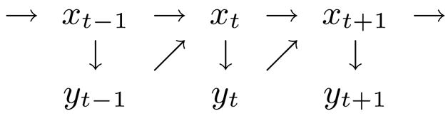
Graphical model of the statistical relationship between the states and the outputs of the closed-loop system. The dependence on the deterministic inputs has been suppressed for clarity.
The complete likelihood function is thus
| (A5) |
This factorization means that, for the purposes of this algorithm, we can regard the feedback as just another input variable. This view corresponds to the direct approach to closed-loop system identification (Ljung, 1999).
The two steps of the EM algorithm for identifying the LDS model in Eqn. 6, when B = D = 0 and C is known, were first reported by Shumway and Stoffer (1982). A more general version, which included estimation of C, was presented by Ghahramani and Hinton (1996). The EM algorithm for the general LDS of Eqn. 6 is a straightforward extension, and we present it here without derivation.
1. E-step
The E-step consists of calculating the following expectations and covariances:
| (A6a) |
| (A6b) |
| (A6c) |
These are computed by Kalman smoothing (Anderson and Moore, 1979), which consists of two passes through the sequence of trials. The forward pass is specified by
| (A7a) |
| (A7b) |
| (A7c) |
| (A7d) |
| (A7e) |
This pass is initialized with and , where π is the estimate for the initial state and Σ is its variance. If there are multiple datasets all initial state estimates are set to π with variance Σ. In fact, these parameters are included in Θ and will be estimated in the M-step.
The backward pass is initialized with and from the last iteration of the forward pass, and is given by
| (A8a) |
| (A8b) |
| (A8c) |
The only quantity that remains to be computed is the covariance Vt+1,t, for which we present a closed form expression:
| (A8d) |
It is simple to show that this expression is equivalent to the recursive equation given by Shumway and Stoffer (1982) and Ghahramani and Hinton (1996).
With the previous estimates of the parameters, Θ^i, and the state estimates from the E-step, it is possible to compute the value of the incomplete log likelihood function using the “innovations form” (Shumway and Stoffer, 1982):
| (A9) |
where are the innovations, their variances, and m is the dimensionality of the output vectors yt.
2. M-step
The quantities computed in the E-step are used in the M-step to determine the argmax of the complete log likelihood Λ (Θ, Θ^i). Using the definitions and the solution to the M-step is given by
| (A10a) |
| (A10b) |
| (A10c) |
| (A10d) |
| (A10e) |
| (A10f) |
where in Eqn. A10c and in Eqn. A10d. The parameters A and B in Eqn. A10e are the current best estimates computed from Eqn. A10c, and C and D in Eqn. A10f are the solutions from Eqn. A10d.
The above equations, except for Eqn. A10a and Eqn. A10b, generalize to multiple datasets. The sums are then understood to extend over all the datasets. For multiple datasets Eqn. A10a is replaced by an average over the estimates of the initial state, x̂1(i), across the N datasets:
| (A11a) |
Its variance includes the variances of the initial state estimates as well as variations of the initial state across the datasets:
| (A11b) |
Footnotes
This transformation only exists if there are n linearly independent eigenvectors, where n is the dimensionality of the state.
Since det B = 0 could result from any singular matrix B, even if B ≠ 0, this test is more stringent than testing B = 0. A singular matrix B implies that some components of the input do not affect the dynamics.
References
- Anderson BDO, Moore JB. Optimal Filtering. Prentice-Hall; Englewood Cliffs, N.J: 1979. [Google Scholar]
- Baddeley RJ, Ingram HA, Miall RC. System identification applied to a visuomotor task: Near-optimal human performance in a noisy changing task. J Neurosci. 2003;23(7):3066–3075. doi: 10.1523/JNEUROSCI.23-07-03066.2003. [DOI] [PMC free article] [PubMed] [Google Scholar]
- Baraduc P, Wolpert DM. Adaptation to a visuomotor shift depends on the starting posture. J Neurophysiol. 2002;88(2):973–981. doi: 10.1152/jn.2002.88.2.973. [DOI] [PubMed] [Google Scholar]
- Clamann HP. Statistical analysis of motor unit firing patterns in a human skeletal muscle. Biophys J. 1969;9(10):1233–1251. doi: 10.1016/S0006-3495(69)86448-9. [DOI] [PMC free article] [PubMed] [Google Scholar]
- Dempster AP, Laird NM, Rubin DB. Maximum likelihood from incomplete data via the EM algorithm. J Royal Statistical Society, Series B. 1977;39:1–38. [Google Scholar]
- Donchin O, Francis JT, Shadmehr R. Quantifying Generalization from Trial-by-Trial Behavior of Adaptive Systems that Learn with Basis Functions: Theory and Experiments in Human Motor Control. J Neurosci. 2003;23(27):9032–9045. doi: 10.1523/JNEUROSCI.23-27-09032.2003. [DOI] [PMC free article] [PubMed] [Google Scholar]
- Draper NR, Smith H. Applied regression analysis. 3 Wiley; New York: 1998. [Google Scholar]
- Efron B, Tibshirani RJ. An Introduction to the Bootstrap. Chapman & Hall; New York: 1993. [Google Scholar]
- Favilla M, Hening W, Ghez C. Trajectory control in targeted force impulses. VI. Independent specification of response amplitude and direction. Exp Brain Res. 1989;75(2):280–294. doi: 10.1007/BF00247934. [DOI] [PubMed] [Google Scholar]
- Flanagan JR, Rao AK. Trajectory adaptation to a nonlinear visuomotor transformation: evidence of motion planning in visually perceived space. J Neurophysiol. 1995;74(5):2174–2178. doi: 10.1152/jn.1995.74.5.2174. [DOI] [PubMed] [Google Scholar]
- Ghahramani Z, Hinton GE. Parameter estimation for linear dynamical systems. Technical Report CRG-TR-96-2; University of Toronto, Department of Computer Science, 6 King’s College Road, Toronto, Canada M5S 1A4. 1996. [Google Scholar]
- Good PI. Permutation tests: a practical guide to resampling methods for testing hypotheses. 2 Springer Verlag; New York: 2000. [Google Scholar]
- Gordon J, Ghilardi MF, Cooper SE, Ghez C. Accuracy of planar reaching movements. II. Systematic extent errors resulting from inertial anisotropy. Exp Brain Res. 1994;99(1):112–130. doi: 10.1007/BF00241416. [DOI] [PubMed] [Google Scholar]
- Harris CM, Wolpert DM. Signal-dependent noise determines motor planning. Nature. 1998;394(6695):780–784. doi: 10.1038/29528. [DOI] [PubMed] [Google Scholar]
- Hay JC, Pick HL. Visual and proprioceptive adaptation to optical displacement of the visual stimulus. J Exp Psychol. 1966;71(1):150–158. doi: 10.1037/h0022611. [DOI] [PubMed] [Google Scholar]
- Held R, Gottlieb N. Technique for studying adaptation to disarranged hand-eye coordination. Percept Mot Skills. 1958;8:83–86. [Google Scholar]
- Houde JF, Jordan MI. Sensorimotor Adaptation in Speech Production. Science. 1998;279(5354):1213–1216. doi: 10.1126/science.279.5354.1213. [DOI] [PubMed] [Google Scholar]
- Jordan MI, Rumelhart DE. Forward models – supervised learning with a distal teacher. Cognitive Science. 1992;16(3):307–354. [Google Scholar]
- Kailath T. Linear Systems. Prentice-Hall; Englewood Cliffs, NJ 07632: 1980. [Google Scholar]
- Krakauer JW, Pine ZM, Ghilardi MF, Ghez C. Learning of visuomotor transformations for vectorial planning of reaching trajectories. J Neurosci. 2000;20(23):8916–8924. doi: 10.1523/JNEUROSCI.20-23-08916.2000. [DOI] [PMC free article] [PubMed] [Google Scholar]
- Lackner JR, Dizio P. Rapid adaptation to coriolis force perturbations of arm trajectory. J Neurophysiol. 1994;72(1):299–313. doi: 10.1152/jn.1994.72.1.299. [DOI] [PubMed] [Google Scholar]
- Ljung L. System Identification: Theory for the User. 2 Prentice Hall PTR; Upper Saddle River, NJ 07458: 1999. [Google Scholar]
- Matthews PB. Relationship of firing intervals of human motor units to the trajectory of post-spike after-hyperpolarization and synaptic noise. J Physiol. 1996;492:597–628. doi: 10.1113/jphysiol.1996.sp021332. [DOI] [PMC free article] [PubMed] [Google Scholar]
- Miles F, Fuller J. Adaptive plasticity in the vestibulo-ocular responses of the rhesus monkey. Brain Res. 1974;80(3):512–516. doi: 10.1016/0006-8993(74)91035-x. [DOI] [PubMed] [Google Scholar]
- Norris S, Greger B, Martin T, Thach W. Prism adaptation of reaching is dependent on the type of visual feedback of hand and target position. Brain Res. 2001;905(12):207–219. doi: 10.1016/s0006-8993(01)02552-5. [DOI] [PubMed] [Google Scholar]
- Pine ZM, Krakauer JW, Gordon J, Ghez C. Learning of scaling factors and reference axes for reaching movements. Neuroreport. 1996;7(14):2357–2361. doi: 10.1097/00001756-199610020-00016. [DOI] [PubMed] [Google Scholar]
- Redding G, Wallace B. Effects on prism adaptation of duration and timing of visual feedback during pointing. J Mot Behav. 1990;22(2):209–224. doi: 10.1080/00222895.1990.10735511. [DOI] [PubMed] [Google Scholar]
- Scheidt R, Dingwell J, Mussa-Ivaldi F. Learning to move amid uncertainty. J Neurophysiol. 2001;86(2):971–985. doi: 10.1152/jn.2001.86.2.971. [DOI] [PubMed] [Google Scholar]
- Shumway RH, Stoffer DS. An approach to time series smoothing and forecasting using the EM algorithm. J Time Series Analysis. 1982;3(4):253–264. [Google Scholar]
- Soechting JF, Flanders M. Errors in pointing are due to approximations in sensorimotor transformations. J Neurophysiol. 1989;62(2):595–608. doi: 10.1152/jn.1989.62.2.595. [DOI] [PubMed] [Google Scholar]
- Thoroughman KA, Shadmehr R. Learning of action through adaptive combination of motor primitives. Nature. 2000;407:742–747. doi: 10.1038/35037588. [DOI] [PMC free article] [PubMed] [Google Scholar]
- Todorov E, Jordan M. Optimal feedback control as a theory of motor coordination. Nat Neurosci. 2002;5(11):1226–1235. doi: 10.1038/nn963. [DOI] [PubMed] [Google Scholar]
- von Helmholtz H. Handbuch der physiologischen Optik. Leopold Voss; Leipzig: 1867. [Google Scholar]
- Weber RB, Daroff RB. The metrics of horizontal saccadic eye movements in normal humans. Vision Res. 1971;11(9):921–928. doi: 10.1016/0042-6989(71)90212-4. [DOI] [PubMed] [Google Scholar]
- Welch RB, Choe CS, Heinrich DR. Evidence for a three-component model of prism adaptation. J Exp Psychol. 1974;103(4):700–705. doi: 10.1037/h0037152. [DOI] [PubMed] [Google Scholar]
- Wolpert DM, Ghahramani Z, Jordan MI. Are arm trajectories planned in kinematic or dynamic coordinates? An adaptation study. Exp Brain Res. 1995;103(3):460–470. doi: 10.1007/BF00241505. [DOI] [PubMed] [Google Scholar]