

Abstract
The sensorimotor calibration of visually-guided reaching changes on a trial-to-trial basis in response to random shifts in the visual feedback of the hand. We show that a simple linear dynamical system is sufficient to model the dynamics of this adaptive process. In this model, an internal variable represents the current state of sensorimotor calibration. Changes in this state are driven by error feedback signals, which consist of the visually perceived reach error, the artificial shift in visual feedback, or both. Subjects correct for at least 20% of the error observed on each movement, despite being unaware of the visual shift. The state of adaptation is also driven by internal dynamics, consisting of a decay back to a baseline state and a “state noise” process. State noise includes any source of variability that directly affects the state of adaptation, such as variability in sensory feedback processing, the computations that drive learning, or the maintenance of the state. This noise is accumulated in the state across trials, creating temporal correlations in the sequence of reach errors. These correlations allow us to distinguish state noise from sensorimotor performance noise, which arises independently on each trial from random fluctuations in the sensorimotor pathway. We show that these two noise sources contribute comparably to the overall magnitude of movement variability. Finally, the dynamics of adaptation measured with random feedback shifts generalizes to the case of constant feedback shifts, allowing for a direct comparison of our results with more traditional blocked-exposure experiments.
Introduction
Subjects exhibit rapid and robust adaptation in the face of altered feedback in many simple sensorimotor tasks (Held and Gottlieb, 1958; Miles and Fuller, 1974; Welch, 1978; Optican and Robinson, 1980). When studying these forms of plasticity a fundamental question arises: How does sensory feedback drive learning? We address this problem from a psychophysical and modeling perspective using reach adaptation to shifted visual feedback. Traditionally, studies of reach adaptation have employed a blocked experimental design, where adaptation is quantified by the difference in performance on two blocks of test trials, before and after exposure to shifted feedback (e.g., Held and Gottlieb, 1958; Hay and Pick, 1966; Welch et al., 1974). This blocked design focuses only on the final effects of adaptation, and so it cannot reveal the processes that link sensory feedback in a given trial to the adaptive responses observed in subsequent trials (Nemenman, 2005; Cheng and Sabes, 2006).
Recently, a number of researchers have used analytic techniques from engineering to study the trial-by-trial dynamics of sensorimotor adaptation. These studies found that adaptation occurs rapidly, on the time scale of single trials, when a random shift was added to the visual feedback of the fingertip (Baddeley et al., 2003) or when perturbing forces were introduced during reaching (Thoroughman and Shadmehr, 2000; Scheidt et al., 2001; Donchin et al., 2003). However, subjects in these studies were aware of the experimental manipulations, either due to explicit instructions regarding the visual shift or to the presence of noticeable force perturbations. Therefore, learning likely reflected a combination of automatic sensorimotor processes and strategic cognitive approaches to the task. These two forms of learning obey very different underlying learning rules. For example, when subjects are aware of a shift in visual feedback, they are able to learn much more complex shift patterns then when they are not aware of the shift (Bedford, 1993). The goal of the present study was to quantify the trial-by-trial dynamics of the automatic processes of sensorimotor adaptation, i.e. the processes that are presumably responsible for the ongoing maintenance of sensorimotor calibration. We therefore study the adaptive responses of naïive subjects to surreptitious shifts in visual feedback.
As in previous studies, we model the trial-by-trial dynamics of learning as a linear dynamical system (LDS). However, we make use of the analytic methods described in Cheng and Sabes (2006), which allows us to explore two issues that were not dealt with in earlier studies. First, instead of using least-squares regression to perform model fits, we take a more general maximum likelihood approach. This allows us to build explicit models of the sources of variability in task performance and to fit these models to experimental data. As we will show, such variability plays an important role in the dynamics of adaptation. Second, we consider multiple potential error-feedback signals and attempt to determine which of these signals drive learning.
This study focused on the sequence of reach errors induced by a sequence of visual feedback shifts. We view these errors as a reflection of the underlying state of reach adaptation. By using a random, time-varying sequence of feedback shifts, we obtained a statistically rich sequence of reach errors that was modeled as an LDS (Cheng and Sabes, 2006). We found that this class of models is sufficient to describe the adaptation dynamics: the LDS model captures both the changes in the mean reach endpoint as well as the temporal correlations between these errors and the visual shift.
We draw several conclusions from the resulting model of adaptation dynamics. First, significant adaptation to visual feedback shifts occurs on single trials. Second, we explicitly measure the internal dynamics of adaptation and show that the state of adaptation decays over time. Third, a significant source of movement variability is an internal state noise which directly affects the state of adaptation, and therefore accumulates across trials. This form of variability only indirectly affects the performance on a particular trial. We show that the state noise accounts for at least a quarter of the overall movement variability. This offers a very different perspective on the sources of movement variability.
Finally, to relate these results to previous research using the blocked experimental design, we used the model derived from stochastic feedback trials to predict the sequence of reach errors induced by blockwise-constant feedback shifts. We find that the adaptation dynamics generalizes across feedback shift conditions. We conclude that the dynamics of adaptation are not specific to the sequence of feedback shifts and that the LDS model can provide insight into the general mechanisms of reach calibration.
Materials and Methods
Experimental setup and data collection
This study was approved by the University of California, San Francisco Committee on Human Research, and subjects gave informed consent. Ten right-handed subjects (four male, six female, 18–28 years-old) with no known neurological history and normal or corrected-to-normal vision participated in this study. Subjects were naïve to the purpose of the experiment and were paid for their participation.
The experiment consisted of trials in which subjects reached toward visual targets with their right arm with virtual visual feedback (Fig. 1A). Throughout each session, the right arm remained on or just above a horizontal table with direct view of the arm (and the rest of the body) occluded by a mirror and a drape. The right wrist was fixed with a brace in the neutral, pronate position, and the index finger was extended and fixed with a splint. An infrared-light-emitting diode was attached to the tip of the index finger, and its position was recorded at 200Hz with an Optotrak infrared tracking system (Northern Digital, Waterloo, Ontario). Since the subject’s hand was essentially restricted to a two-dimensional workspace, we analyzed only two components of the recorded positions: the positive x-axis points right and the positive y-axis points sagittally away from the subject.
FIG. 1.

A: Virtual feedback setup. B: Definition of reach and feedback variables: f, location of unseen fingertip location at end of reach; c, location of visual feedback (cursor); g, target location; e, true reach error; υ, visually perceived reach error; p, artificial feedback shift (perturbation).
Target positions and virtual visual feedback of the fingertip location (when it was available) were generated by a liquid crystal display projector (1024 × 768 pixels, 75 Hz) and viewed in the mirror via a rear-projection screen which was placed so that projected images appeared to lie in the plane of the table, at the vertical level of the fingertip. In some trials, the visual feedback was shifted relative to the true location of the fingertip, as described below. All subjects reported being unaware of any such feedback manipulation in a post-experiment questionnaire.
Task design
The purpose of this experiment was, first, to identify the adaptation dynamics in response to stochastic feedback shifts (Stoch-p) and, second, to compare the dynamics to those observed in trial blocks with constant feedback shift (Const-p), the traditional paradigm for inducing adaptation.
An experimental session consisted of four repetitions of the following sequence of trial blocks: 25 transition trials (see below), 35 Const-p trials, 10 transition trials, and 50 Stoch-p trials. Within each Const-p trial block the feedback shift was constant, but the shift varied between the four Const-p block. The four shifts were a random ordering of the four vectors with ±3 cm along both the x- and y-axes. Transition trials with either unshifted visual feedback or no visual feedback were inserted in order to minimize the possibility that subjects became aware of manipulations in the visual feedback. Each Const-p trial block was preceded by 15 trials with unshifted feedback and then 10 trials without visual feedback. When a Const-p block followed a Stoch-p block, the shift was ramped down to zero over the the first five of these transition trials. Each Const-p block was also followed by 10 trials without visual feedback. In total, each session consisted of 480 trials, with 200 Stoch-p trials and 140 Const-p trials. An example session is shown in (Fig. 2).
FIG. 2.
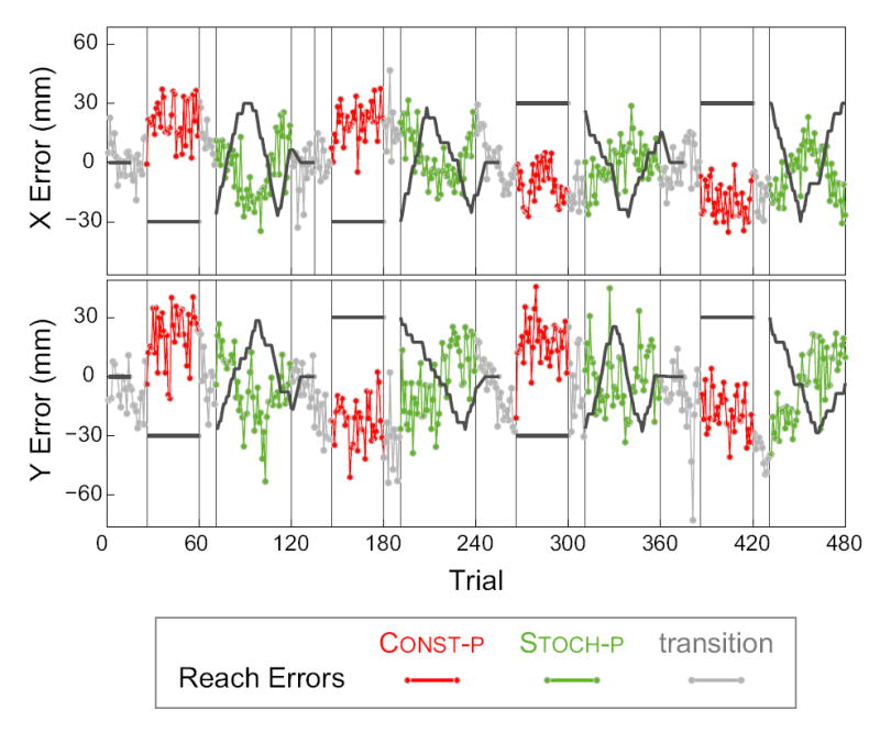
An example trial sequence. Visual feedback shifts (black traces) and reach errors (see key at bottom) along the X-axis (top panel) and Y-axis (bottom panel) are shown. Gray vertical bars mark boundaries between blocks of trial types: Stoch-p: stochastically shifted feedback; Const-p: constant feedback shift; transition: trials include reaches without visual feedback to prevent subjects from noticing onset of constant shift blocks and ramping down of shift after a Stoch-p block.
Stochastic feedback-shift sequence
We expect that reach adaptation will be driven by either the artificial shifts in visual feedback, the resulting visually perceived reach errors, or a combination of both. In other words, these signals will be the “inputs” that drive changes in the state of adaptation. To identify the trial-by-trial dynamics of adaptation, these inputs have to be “rich” enough to excite all the modes of the dynamics (e.g. Ljung, 1999). Feedback shifts that follow a white-noise sequence would be ideal, especially because they decorrelate the input sequence and the state (Cheng and Sabes, 2006). However, in pilot experiments subjects often became aware of these shifts, creating the possibility of explicit cognitive strategies. Therefore, we used a modified random walk sequence of visual shifts for this study.
From one trial to the next, the shift in visual feedback (p, see Fig. 1B) changed incrementally by one of the following (x, y) vectors, selected with equal probability: (0, 0), (0, sy), (sx, 0), or (sx, sy)/√2, where |sx| = |sy| = 5.2 mm, and the initial sign of sx and sy were assigned randomly at the beginning of each block. The maximum magnitude of the feedback shift in either dimension was limited to ±3 cm. If the increment selected would have caused the x or y component of the feedback shift to exceed this range, then the sign of sx or sy, respectively, was reversed (reflecting boundaries). In each trial block, the feedback shift in the first trial was the value used in the last preceding trial with feedback. Example random walk sequences are shown in the Stoch-p blocks of Fig. 2.
Reach Trials
Every trial in the experiment consisted of reaching to a visual target. At the beginning of each of these trials, subjects were guided to a start position without visual feedback about either the start location or their hand (“arrow field” technique, Sober and Sabes, 2005). Specifically, an array of 3 × 3 identical arrows appeared in a randomized position of the workspace. The arrows corresponded to the vector from the current finger position to the start position, with a maximal length of 9 cm. Subjects were instructed to move their finger in the direction indicated by the orientation of the arrows until the arrows disappear, which occurred when the fingertip was within 5 mm of the unmarked start position. The start position was the same for all trials and was located a few centimeters in front of the subject, roughly along the midline.
Subjects were required to hold the start position for a random delay (0.5–1 s) until the reach target appeared (an open green circle, radius 6 mm). The target location gt was drawn randomly from a uniform distribution over a 4 cm square centered 26 cm distally from the start location. The appearance of the target together with an audible tone were the go-signal for initiating the reach. Subjects were instructed to make a single quick and smooth movement towards the target. The trial terminated when the velocity of the finger fell below 2 mm/s.
In order to minimize variation in movement speed across trials, a loose timing constraint was used. The movement duration was defined as the length of the time interval between when the finger first moved more than 1 cm from the start location and when the tangential velocity of the finger first fell below 15% of its peak value at the end of the movement. These landmarks were chosen to exclude effects of variable reaction time and movement corrections at the end of the reach. A tone was sounded if reaches were too slow (movement duration > 500 ms) or too fast (movement duration < 300 ms). Subjects generally had no difficulty meeting these criteria.
Subjects received “velocity-dependent terminal feedback”. Visual feedback of the finger tip position appeared only near the end of the movement, when the tangential finger velocity fell below 15% of the peak value, and feedback continued until the end of the trial. This arrangement satisfies two constraints. The feedback appears sufficiently late in the movement so that we are able to assess the endpoint of the initial reach before visual feedback is able to drive corrective changes. The endpoint is thus taken as a measure of the state of the reach adaptation. However, the brief period of visual feedback while the hand is still moving provides a richer feedback signal for learning than would static feedback after the completion of the movement. Feedback was in the form of a white disk, 3 mm radius, located at the fingertip or displaced by the feedback shift p. Finally, subjects were instructed to correct any reach errors after completing the first reach, and trials terminated when the finger remained stationary within the target circle for 500 ms.
In some transition trials subjects received no visual feedback of their reaching arm during any part of the trial. These trials were identical to those with visual feedback, except that the target was marked by a filled green circle with radius 6 mm, providing a cue of the feedback type prior to reach initiation.
Prior to data collection subjects were given sufficient practice trials to ensure that all task constraints were met.
Data analysis and a model for the dynamics of adaptation
Velocities were determined by first order numerical differentiation of the positional data after smoothing with a 5 Hz low-pass Butterworth filter. The reach endpoint, ft, on trial t was defined as the finger position when the tangential velocity first fell below 5% of its maximum value on that trial. Typical velocity profiles were unimodal bell-shaped curves (cf. Atkeson and Hollerbach, 1985), corresponding to the primary reaching movement, followed by one or more smaller peaks due to corrective movements. In a few trials the velocity fell below 5% criterion only after the second velocity peak. In these cases visual inspection usually indicated a clear endpoint for the primary reach (velocity dip and curvature peak), however, in the rare cases where an endpoint could not be identified confidently the trial was discarded. The reach error et is defined as the difference between the target position gt and the reach endpoint ft (Fig. 1B), et ≡ ft − gt.
We use a linear dynamical systems (LDS) model to describe the adaptation dynamics (Scheidt et al., 2001; Donchin et al., 2003; Cheng and Sabes, 2006). The output of the system, yt, is a noisy readout of the internal state of the sensorimotor map, xt. Here we define yt to be the reach error, et. This means that the internal state of the system is defined as the mean reach error one would observe across trials if adaptation could be frozen in time. Given the limited set of reach vectors used in this experiment, the state can be described with a single two-dimensional variable. Formally we write,
| (1a) |
where rt is the sensorimotor noise, or output noise, in trial t, assumed to be an independent zero-mean, Gaussian random variable with a covariance matrix R, i.e. rt ~ N (0, R). We model adaptation as the trial-by-trial change in x due to sensory feedback on the preceding trial. Formally,
| (1b) |
where ut are the sensory feedback variables (inputs) driving adaptation, and qt is additive noise in the state variable, assumed to be independent, zero-mean, Gaussian with covariance Q, i.e. qt ~ N (0, Q). The term But represents error corrective learning, Axt represent the decay of the state of adaptation back to baseline, and qt represents variability in these two processes. Since the spatial variables are all two-dimensional vectors, the parameters of the LDS model, A, B, Q, and R are 2×2-matrices. There are no direct “feedthrough” inputs affecting yt, since terminal visual feedback prevents online visual correction and the ongoing reaches were not otherwise externally perturbed.
An important variable in the LDS model of Eqn. 1 is the feedback signal that drives adaptation, ut. Our experimental design makes the selection of candidate signals easier, since visual feedback is given only near the end of the movement, and it only represents the location of the index fingertip (Fig. 1B). Under these conditions, there are two likely candidates for the input signal: the visually perceived error υ defined as the difference between the position of the visual feedback at the reach endpoint and the target position, υt ≡ ct − gt, and the artificial feedback shift, pt (Fig. 1B). We also consider the reach error, e, as a potential input signal. Note that the three error signals are linearly related: et = υt − pt. Therefore, any model which includes two of these variables effectively includes the third one as well.
Given a sequence of inputs ut and outputs yt, the maximum likelihood estimate of the model parameters A, B, Q, and R are determined using an expectation-maximization algorithm (EM) (Shumway and Stoffer, 1982; Ghahramani and Hinton, 1996; Cheng and Sabes, 2006). Matlab routines for performing this analysis are freely available at http://keck.ucsf.edu/~sabes/software/. The algorithm takes into account that data was collected in separate blocks by resetting the state to an initial Gaussian distribution (with the necessary additional model parameters) at the beginning of each block. The EM algorithm is only guaranteed to converge to a local maximum of the log likelihood. In fact, however, we find that the parameter estimates were robust to running the estimation algorithm with different sets of initial values, suggesting that no local minima exist close to the identified parameter estimates.
The EM algorithm will find a maximum likelihood model for any input and output sequence. Therefore, it is important to be able to assess model performance. We begin with model selection, asking whether particular model parameters, in this case input signals, provide significant explanatory power. We then describe two approaches to quantifying whether the best-fit model is sufficient to account for important statistical features of the input-output sequences. These analyses are described in detail below.
Likelihood Ratio Test for model selection
To determine whether the inclusion of a particular input variable or other parameter provides significant explanatory power we use the generic likelihood ratio test (LRT) for maximum likelihood estimation (Stuart and Ord, 1987). Consider a model class M1 with v1 free parameters and a second model class, M0, with a subset of free parameters, v0 < v1. For example, M1 could be the model with a particular two-dimensional input variable ut, and M0 could be the null model with no input variables. M0 has four fewer free parameters, since it has no input weighting matrix B. Given each model class, we can find the maximum likelihood model parameters and the values of likelihood they achieve, Li for model Mi. The inclusion of additional model parameters will always result in a better fit to the data, i.e., L1 > L0. However, under the assumption that the data come from a model in M0, the distribution of gains in log likelihood due only to overfitting is known in the limit of large datasets:
| (2) |
Using this distribution, the LRT either accepts or rejects the additional parameters.
Predicting the statistics of the reach errors
The most direct approach to assessing model sufficiency would be to compare the empirical output sequence yt with the outputs predicted from the model and the input sequence. However, the outputs depend heavily on the specific sequence of state noise terms, qt, which are not directly observable. Instead, we determine how well models are able to predict the statistics of the sequence of reach errors and its relationship to the sequence of visual shifts.
The sequence of reach errors is characterized by two measures, the variance and the autocorrelation ρe(τ), which is a function of the time lag τ at which the autocorrelation is measured. Similarly, the statistical relationship between the reach error and the visual shift vector is characterized by two measures, the covariance σep and the cross-correlation function ρep(τ). These measures are defined as follows:
| (3a) |
| (3b) |
| (3c) |
| (3d) |
where T is the total number of trials, ā represents the mean value across trials, and aTb represents the inner-product of the vectors a and b.
The statistics defined above provide a summary of the adaptive response of the reach endpoint to the shifted visual feedback. These statistics were not used explicitly when performing the maximum likelihood model fitting. Thus, if the model is able to accurately predict these statistics, then it is sufficient to capture the key elements of the response. The model predictions for these statistics are obtained using a Monte Carlo approach. Given the LDS model parameters and actual sequence of visual shifts experienced by the subject in a given trial block, we simulate a sequence of state and output variables using Eqn. 1, with state and output noise terms generated independently for each simulated trial. For each subject, we compute the desired statistics from 100 combined runs of these Monte Carlo simulations and compare the values to those obtained from the empirical data.
One-step-ahead prediction and the portmanteau test
Our second approach to assessing sufficiency is to test whether an LDS model is demonstrably insufficient to account for the second-order statistics of the sequence of reach errors. We start with the one-step-ahead predictor ŷt, which is the expected value of yt given a model and all the inputs and outputs up to trial t-1. The ŷt are obtained from the Kalman filter using the estimated model parameters (Anderson and Moore, 1979; Shumway and Stoffer, 1982). However, if the LDS model being used to predict the same dataset on which it was fit, a cross-validation procedure is used: the one-step-ahead predictions ŷt for each block of 25 trials are computed using a model fit to the dataset with that block excluded.
If the model captures the adaptation dynamics well, then the one-step-ahead prediction residuals yt − ŷt should be free of temporal correlations, i.e., the residuals should be a white noise sequence. We can compare this null hypothesis to the alternative (significant residual correlations exist) using a portmanteau test for serial autocorrelations (Hosking, 1980). This test is based on the autocorrelations of the prediction errors at a lag of τ trials:
| (4) |
The mth portmanteau statistic combines the autocorrelation at lags up to m trials:
| (5) |
Under the null hypothesis, the model captures the statistical structure of the output sequence, and so the Jτ and (thus) the Pm should be smaller than if the model were not sufficient. In the case of no inputs to the system and in the limit of large T, Pm is χ2 distributed under the null hypothesis (Hosking, 1980). When there are inputs to the system, as is typically the case here, the theoretical distribution of the portmanteau statistic is unknown. Therefore, we use Monte Carlo simulation to estimate the distribution of the portmanteau statistic under the LDS model, given the known sequence of feedback shifts pt. First, we simulate 1000 artificial datasets, as described in the previous section. For each of these artificial datasets we compute the portmanteau statistic, Pm. This yields an empirical distribution of 1000 samples for Pm under the assumption of the LDS model. If the portmanteau statistic calculated from the actual data is larger than the 95th percentile of this distribution, then we reject the null hypothesis and say that the model is not sufficient to account for the sequence of reach errors.
While the portmanteau test can be used for any maximum lag m, the statistical power of the test decreases with the lag (Davies and Newbold, 1979). On the other hand, larger lags need to be included in the portmanteau statistic to test for long-range residual auto-correlations. As a compromise, we will present the portmanteau statistic for maximum lags m up to 8 trials, although no substantial differences were noted for for maximum lags up to 20 trials.
Results
We are primarily concerned with the trial-by-trial sequence of reach errors, which reflects the changing state of reach adaptation. A sequence from a typical session is shown in Fig. 2. Two salient features of these plots highlight the key elements of the the dynamics of adaptation. First, over the course of a block, the reach errors are strongly influenced by the direction of the visual feedback shift: the error appears to roughly track the inverse of the shift. This is the general pattern that is expected when subjects adapt to the shifted feedback. Second, there is considerable variability in reach error from one trial to the next trial, even when there is no time-varying feedback shift.
The goal of this work is to quantify and characterize how such error sequences arise from a combination of error corrective learning processes and the various sources of variability, including a stochastic component of the internal dynamics of adaptation. In the rest of this paper we employ the LDS model of adaptation in order to accomplish this goal.
Error Corrective Learning
We begin by determining which feedback signals, if any, drive error corrective learning. In terms of the LDS model, this means identifying the inputs that lead to a significantly better fit to the data. The three candidate inputs signals each have a corresponding LDS update (learning) equation,
| (6) |
that represent three classes of LDS models. Two additional model classes are also considered: the null model class,
| (7) |
which has no error feedback, and the Mυp model class, in which both υ and p contribute to reach adaptation. Since υ, p, and e are linearly related, Mυp is equivalent to any model that includes at least two of the three input signals. Together, these five model classes form the hierarchy shown in Fig. 3.
FIG. 3.

Hierarchical model selection. Arrows represent comparisons between nested model classes (boxes) made with the likelihood ratio test (LRT) on Stoch-p data. Each test had four degrees-of-freedom, corresponding to 2×2 matrix parameters. p-values for the LRT, shown next to the appropriate arrow, apply across all 10 subjects and were highly consistent. Thick lines represent comparisons for which the additional input variable resulted in a significant improvement
We use the likelihood ratio test (LRT) to compare each pair of models that differs by the inclusion of a single variable (arrows in the hierarchy of Fig. 3). For each subject, each model class was fit to the sequence of 200 reach errors from the 4 Stoch-p trial blocks. Both the visually perceived error υ and the feedback shift p significantly improved the fit over the null model for every subject. In contrast, including the reach error e did not significantly improve the model for any subjects. These results indicate that the trial-by-trial changes in reach error are not simply the result of a random walk. Rather, we observe an error-corrective adaptation process driven by either the visually perceived error, the feedback shift, or a combination of both.
The relative contributions of these two feedback signals could, in principle, be quantified with the LDS approach. However, there is not sufficient statistical power to accomplish this when there is a strong correlation across trials between the two signals. In our case, the visually perceived error and the feedback shift are related by the expression υt = et + pt, and so we expect them to be correlated. Indeed, across subjects the mean (± std.) correlation coefficient between υ and p in the Stoch-p trial blocks is 0.35 ± 0.12. It is, therefore, not surprising that while both the Mυ and Mp single-input models are significant, the two-input model Mυp does not yield a significant improvement over either. The same qualitative results is obtained when the model selection procedure is applied to artificial data generated with the best-fit Mυ or Mp model, underscoring the lack of power to quantify the relative roles of the two feedback signals. Thus, in the remainder of the paper we will analyze both the Mυ and Mp model classes.
Model parameters
We next consider the maximum likelihood parameter values for the Mυ and Mp model classes (Fig. 4). We will show that the learning rates are quite large, with subjects correcting for about one-third of the error feedback after each trial. We will also show that the parameters governing state decay (“forgetting”), state noise, and output noise suggest an important role for each of these processes. Finally, we will show that while the values for these latter parameters differ between the Mυ and Mp model fits, the two model classes are nearly equivilant from the perspective of these datasets.
FIG. 4.

Maximum likelihood LDS model parameters. Best fit parameters for the Mυ and Mp models. Each panel represents the values of a 2 × 2-matrix parameter (see label on y-axis), with values for all subjects clustered by the matrix component: . Bar colors correspond to subjects (n = 10).
The best-fit values of the of the learning parameter, B, agree quite well between the two model classes (Fig. 4). In order to interpret these 2 × 2 matrices, we consider the first (second) eigenvalues of B, which represent the maximum (minimum) fraction of the error feedback that is corrected for, depending on the direction of the error vector. The mean and standard deviation of the eigenvalues of B (and the other model parameters) are shown in Table I. They represent a per-trial correction of the respective error signals (υ or p) in the range of 20-50%, across subjects, a rapid pace of learning.
TABLE I.
Mean (± std.) eigenvalues for the LDS model parameters. Eigenvalues for each 2 × 2 matrix parameter were sorted in descending order and then averaged across subjects. For Q and R, the square-root of the eigenvalues was used, and so the parameters represent standard deviations and have units of mm. A and B are dimensionless.
| Mυ | Mp | |
|---|---|---|
| A | [0.97 0.89] ± [0.03 0.09] | [0.77 0.52] ± [0.13 0.23] |
| B | [-0.36 -0.18] ± [0.18 0.10] | [-0.38 -0.18] ± [0.18 0.10] |
| [8.7 4.2] ± [4.4 2.4] | [6.2 2.5] ± [3.4 1.18] | |
| [12.3 9.1] ± [5.1 3.2] | [14.6 11.0] ± [5.5 4.1] |
The most pronounced difference between the two model fits is in the value of the “decay” parameter, A. The values of A are larger for the Mυ model than for the Mp model, and there is markedly greater consistency across subjects for the Mυ model. The first (second) eigenvalues of A represent the maximum (minimum) fraction of the state xt that has not decayed back to the mean by the next trial, ignoring the inputs u. A value of 1 means no state decay (no forgetting), and a value of 0 means a complete reset of the state after each trial (complete forgetting). For the Mυ model, the maximum eigenvalue of A is 0.97 on average, corresponding to a state-decay half-life of 23 trials (Table I). For the Mp model, the eigenvalues are smaller, with a half-life for the first eigenvector of just three trials.
The parameters Q and R represent the state and output noise, respectively. The best-fit parameter values differ across the two model classes (Fig. 4). However, in both cases the magnitude of the state noise is comparable to that of the output noise. For example, in the Mυ model fit, the standard deviation of the state noise along its most variable axis (first eigenvalue) is 8.7 mm, compared to 12.3 mm for the output noise (Table I). We will return to this comparison later in the paper.
Lastly, we analyze the differences between the Mυ and Mp model fits. It might seem odd that the models agree so closely on the learning parameter B, which is applied to different input signals in the two models, while they disagree on the state decay parameter A. Yet, these differences are expected given the relationship between the visually perceived error υ and the feedback shift p. To show this we rewrite the state update equations for the two models (Eqn. 6) using the LDS output (Eqn. 1a) and the fact that et is the LDS output:
| (8) |
where subscripts have been added to the parameter variables for clarity. When the noise term Bprt is relatively small, the two models are essentially the same if the two equalities Bυ = Bp and Aυ = Ap − Bp hold. Even if Bprt is not small, however, that term only contributes to the effective state noise, and so these equalities should hold whenever the Mυ and Mp models are fit to the same dataset. Indeed, the best fit values of B for the two model classes are nearly identical (Fig. 4 and Table I), and across subjects the mean (± std.) value of the expression Aυ − (Ap − Bp) is
This analysis shows that the Mυ and Mp model classes are essentially equivalent, formally differing only in structure of the noise terms. Since in the following we focus on these noise terms, we will continue to present results for both model classes, as they represent endpoints in the continuum of models in which both signals contribute with varying strengths.
Model sufficiency
In the two previous sections, we showed that the visually perceived reach error and/or the visual feedback shift drive a large and significant adaptive response. Here we ask whether our LDS models of that response are sufficient, that is, whether they do “good enough a job” of explaining the trial-by-trial sequence of reach errors.
Sample data
Figure 5 shows the sequence of reach errors in the Stoch-p trial blocks for a single subject. In addition, this figure shows one-step-ahead model predictions for three different models, i.e. the predicted reach errors for each trial given the actual inputs and outputs up to the previous trial. The one-step-ahead predictions of the best-fit Mυ and Mp models (Fig. 5, red and blue traces, respectively) largely overlap each other, as expected. These predictions appear to track the errors well, capturing the general trends in the data. However, two other features of these traces should be noted. First, while according to the LRT the Mυ and Mp models fit the data significantly better than the null model, M0̸ (black trace), the difference in the one-step-ahead predictions are rather small. This is due to the fact that the predictor is using all inputs and outputs up to a given trial to predict the output on the next trial. Second, all three models leave a large residual of unpredicted reach error in this sample dataset.
FIG. 5.
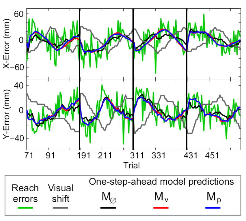
Sample model predictions. Reach errors and one-step-ahead model predictions for one subject in the Stoch-p trial blocks.
In the remainder of this section we present two approaches to assessing model sufficiency, one addressing the shortcomings of the one-step-ahead predictor and one aimed at the prediction residuals. First we determine how well the models predict the statistical relationship between the reach error and the visual shift. Unlike the one-step-ahead predictor, these predictions are made without access to the real sequence of reach errors, making them a much more stringent test of model sufficiency. Secondly, we examine the one-step-ahead residuals in order to determine whether they are as good as can be expected, given the levels of state and output noise, or whether there is still some “signal” to be accounted for.
Predicting reach error statistics
Our first test of model sufficiency is how well a model predicts the statistical structure of the adaptive response to shifted feedback. As described in the Methods, we chose four statistical measures: the variance and autocorrelation of the reach errors and the covariance and cross-correlation between the reach errors and feedback shifts Eqn. 3d). For each subject, we computed these measures from the empirical sequence of reach errors in the Stoch-p trial blocks. We also computed the measures from 100 combined Monte Carlo simulations of that sequence, generated from the best-fit LDS model and the true sequence of visual feedback shifts (see Methods).
We first observe that the Mυ and Mp models provide a nearly perfect account of the reach variance and autocorrelation (Fig. 6A,B). However, the null model M0̸ performs just as well by these measures. This result shows that the state decay A, state noise Q, and output noise R parameters of the LDS are sufficient to account for the second-order statistics of the reach errors. Furthermore, it shows that the maximum likelihood fitting procedure implicitly fits these quantities.
FIG. 6.

The linear dynamical system (LDS) model is sufficient to predict the statistical structure of the adaptive response to shifted feedback. A: Comparison of empirical reach error variance and the predicted variance under the best-fit Mυ (black), Mp (green), and M0̸ (red) models. Datapoints represent values for a single subject (symbols overlap), and thick lines represent a linear regression of empirical data on prediction (p < 0.05). B: Reach error auto-correlation function ρe (τ) for time lags τ = 1–8 trials. The dark gray band represents mean ± sem. across subjects. Model predictions are shown in three lines representing mean ± sem. across subjects: Mυ, green; Mp, black; M0̸ red. C: Comparison of empirical values and model predictions of the covariance σep between reach errors and visual shifts. Symbols as in A. D: Cross-correlation function ρep (τ) between reach errors and feedback shifts, along with the Monte Carlo model predictions. Symbols as in B. E: Sensitivity analysis: how predicted cross-correlation functions depend on model parameters. The gray band (data) green line (Mυ model predictions) are the same as those in panel B. The other colored lines represent the cross-correlations predicted by the best-fit Mυ model with selected parameters altered, as indicated by the legends. Only the diagonal elements of the parameter matrices A and B were varied, while in the case of Q and R the entire matrix was scaled.
Next we consider the relationship between the reach errors and the sequence of visual feedback shifts. For all subjects, there is a large negative covariance between these variables (Fig. 6C), as expected when subjects adapt their reach error to the visual shift. The predicted covariance under the best-fit Mυ and Mp models are nearly identical to each other. While there is a slight downward bias (weaker correlation) in the model predictions, discussed further below, the predicted and empirical values are strongly correlated across subjects. In contrast, the null model predicts essentially no covariance between the reach error and visual shift. The Mυ and Mp model models also provide an excellent prediction of the cross-correlation function between the sequences of reach errors and visual shifts (Fig. 6D).
The close agreement between the empirical and predicted error-shift cross-correlation functions raises the question of how sensitive a measure this is. We want to be sure that the predictions depend on the details of the model and are not, for example, dominated by the sequence of visual shifts. Therefore, we performed a sensitivity analysis to quantify how the predicted cross-correlation function depends on the model parameters. We generated Monte Carlo simulations with individual parameters altered from their actual best-fit values. The predicted cross-correlations were found to be sensitive to all four parameters, and even fairly small parameter changes can produce large discrepancies between the data and model predictions (Fig. 6E, only results for Mυ are shown).
Residuals of one-step-ahead predictions
If the one-step-ahead model predictions captured the full dynamics of adaptation, then the residual errors should have no statistical structure, i.e. they should be white noise. This can be assessed by the portmanteau test for serial autocorrelations. If significant correlations existed in the model prediction residuals, then the model would be insufficient to account for the dynamics of adaptation, and the model would be rejected. For all subjects, the one-step-ahead predictions of both the Mυ and the Mp model leave no significant residual correlations in a cross-validation test for the Stoch-p trial blocks (portmanteau test, p > 0.05, max. lag m = 8).
These results suggest that the LDS models are sufficient to capture the trial-by-trial dynamics of adaptation. However, since the portmanteau test pools all residuals and all time-lags into a single statistic, it has relatively low statistical power. This means that more subtle model inaccuracies might not be detectable with this approach. Detecting such inaccuracies is especially important when interpreting the state and output noise terms, since model inaccuracies will appear in our model fits as additional noise. Therefore, we performed a variety of additional analyses on the model residuals, testing for violations of normality, stationarity, and model linearity. We found no significant evidence for any of these effects, as described in detail in the Appendix.
Together, these analyses suggest that the LDS models considered here are indeed sufficient to explain the dynamics of reach adaptation in the Stoch-p trial blocks.
State noise
The two sources of variability in the LDS model, the state noise and the output (or sensorimotor) noise, are conceptually quite different and both will contribute to the overall variability in any measure of performance. While the output noise is uncorrelated across trials, state noise is accumulated in the state and, hence, its contribution to the reach variability is correlated across trials. Given that the state noise is often overlooked in models of motor variability, we want to confirm here that the level of state noise is indeed significant.
We use the LRT to compare the Mυ or Mp model class to a null hypothesis class with no state noise. In practice, Q cannot vanish entirely, or the parameter estimation algorithm would become unstable. Hence, for the null hypothesis we use a model with the state noise covariance fixed to a negligible value (Q = 0.1mm2) relative to the output noise covariance R. The LRT shows that the addition of state noise significantly improves the model fit in the Stoch-p condition for both learning models and for all subjects (Mυ: p < 10−4; Mp: p < 0.003; N = 10).
We confirm this result by applying the portmanteau test to the best-fit null hypothesis model (i.e. the best model with Q = 0.1mm2). These models could not capture the temporal structure of the reach errors: the residuals were significantly correlated across trials (Mυ rejected in 10/10 subjects, Mp rejected in 7/10; p < 0.05, max. lag m = 8). These results establish that state noise contributes significantly to the trial-by-trial sequences of reach error.
Next, we assess the magnitude of the state noise by comparing it to the output noise. As a measure we choose the ratio of the largest eigenvalues of the state and output covariance matrices, υQ and υR respectively, (see also Table I):
| (9) |
For all subjects, the two noise terms are on the same order of magnitude, although the output is typically larger by about a factor of two (Fig. 7, open bars). To assess the statistical significance of the ratio k, we compared these values to the 95% confidence values obtained by separately fitting the LDS models to each of 1000 Monte-Carlo simulations run with Q reset to 0.1mm2 (Fig. 7, filled bars). The k ratio obtained in these simulations are quite small (Fig. 7, filled bars), significantly smaller than the values obtained from the true data. This underscores the conclusion that the state noise is an important feature of the data, and not an artifact of the fitting procedure.
FIG. 7.
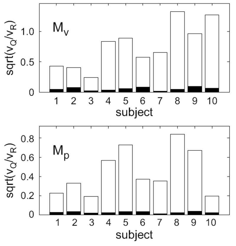
Magnitude of estimated state noise relative to output noise (open bars) for two model classes fit to the Stoch-p data. υQ and υR are the largest eigenvalues of the state and output noise covariances, respectively. Filled bars represent the 95% confidence value under the null hypothesis of negligible state noise determined from 1000 Monte Carlo simulations.
Finally, we consider the contribution of state noise to the overall reach error variability. It is not difficult to show that in the case of no visual feedback shift, the LDS models predict an overall reach variance of
We computed the values of these expressions numerically from the best-fit models. We then quantify the fraction of the overall reach variability that is due to the output noise (the second term in the equations above), as opposed to the state noise (the first term). For the Mυ model there is also a third term corresponding to the effects of feeding the reach error back into the LDS via the input υ. On average, the estimated contribution of state noise to the overall reach error variability was 23% for the Mp model and 38% for the Mυ; error feedback in Mυ contributes another 7%. Therefore, while output noise accounts for more than half of the overall reach endpoint variability, state noise represents a sizable component as well.
Adaptation Dynamics Generalizes to Constant Feedback Shift
Up to this point we have only examined the adaptation dynamics in the Stoch-p trial blocks. One concern that might arise is that the results we have found, e.g. the magnitudes of the learning rates and state noise, are specific to the stochastic sequence of feedback shifts. It is important to verify that the conclusions drawn from studies using these dynamical systems techniques will generalize to other experimental paradigms, in particular to the blocked exposure design traditionally used in studying reach adaptation. Therefore, we quantified how well LDS models that were fit to the Stoch-p data predict the results of the Const-p condition, which is similar to a blocked exposure design. We focused on predictions of the steady-state of adaptation, the statistics of the sequence of reach errors, and the residuals of the one-step-ahead model predictions.
In general, LDS models predict that adaptation should converge to a “steady state” when the input is held constant. However, due to the presence of state and output noise, there will be random fluctuations in both the state and the output even after this convergence has occurred. The LDS model predicts both the magnitude of this steady state reach error and the fluctuations around it. We compared these model predictions to values obtained from the data. The Mυ and Mp models make nearly identical predictions for the steady state error magnitude, and these values correlate well with the empirical data across subjects (Fig. 8A). There is, however, a small bias: the models consistently predict a slightly smaller steady state error than what is empirically observed (mean bias is 2.7 mm for Mυ and 2.8 mm for Mp). Both models make accurate predictions for the standard deviation of the reach error during the steady state (Fig. 8B).
FIG. 8.

Comparison of empirical and predicted steady states of adaptation. Predictions were derived from the Mυ (•, solid lines) and the Mp (◦, dashed lines) models fit to Stoch-p data. Empirical values were averaged over the last 10 trials of each Const-p trial block. A: Magnitude of the steady state of adaption with a 30 cm magnitude shift along each axis. Empirical values are averages of the x and y error coordinates. The expression for model predictions is given in Cheng and Sabes (2006). Linear regression of the measured values on the model fits shown in bold lines (Mυ: R2 = 0.52, p = 0.02; Mp: R2 = 0.50, p = 0.02). B: Standard deviation of the reach error during steady state ( in Eqn. 3a). Model predictions come from Monte Carlo simulations (see Methods). Linear regression in bold lines (Mυ: R2 = 0.79, p = 0.007; Mp: R2 = 0.81, p = 0.006).
Next, we consider how well the Mυ and Mp models fit to the Stoch-p data can predict the statistics of the reach errors across the Const-p trial blocks. Both models provide a good prediction of the variance and autocorrelation of the reach errors as well as the covariance and cross-correlation between the reach errors and the sequence of visual feedback shifts (Fig. 9A-D). This generalization across tasks is not solely due to the nature of the Const-p shift sequence, as the model predictions are sensitive to the parameter values (Fig. 9E).
FIG. 9.

The dynamics model identified from Stoch-p data can also account for adaptation to constant visual shift. Plotting convention is the same as in Fig. 6. A: Reach errors variance vs. Monte Carlo model predictions. B: Auto-correlation function of reach errors for time differences of 1–8 trials and Monte Carlo model predictions. C: Covariance between reach errors and feedback shifts for individual subjects vs. Monte Carlo model predictions. Linear regression of subject data on model prediction was marginally significant: p = 0.06 for the Mυ model (green circles and green regression line) and p = 0.07 for the Mp model (black circles, thick black regression line). D: Cross-correlation function between reach errors and feedback shifts for time differences of 1–8 trials, along with the Monte Carlo model predictions. E: Sensitivity analysis of how predicted cross-correlation functions depend on model parameters.
Finally, however, we note that the generalization is not perfect. We performed the portmanteau test for serial autocorrelations on the residuals of the one-step ahead predictors (models fit on Stoch-p data, tested on Const-p data). For a minority of subjects, the models were unable to fully account for the temporal structure of the reach error sequence (Mυ : fits for 4/10 subjects rejected; Mp : 2/10 rejected; p ≤ 0.05 and max. lag m = 8).
Taken together these comparisons suggest that the dynamics of adaptation largely generalizes from a stochastic sequence of visual shifts to a constant shift paradigm. Furthermore, the LDS model fit to the stochastic shift data are able to quantitatively predict the key features of the of the blocked exposure paradigm.
Discussion
We have shown that the trial-by-trial dynamics of reach adaptation to shifted visual feedback is well described by a simple linear dynamical system. In this model, there are two forces driving changes in the state of adaptation. Firstly, learning is driven by error corrective feedback, with the state of the system correcting for at least 20% of the error observed in the preceding movement, on average. The data presented here are consistent with two candidate error signals: the visually perceived reach error and the artificial visual shift. Secondly, adaptation is driven by the internal dynamics of learning, including a decay back to a baseline state and the accumulation of an internal “learning” or state noise. Finally, the LDS model generalizes from the case of stochastic feedback shifts to the more traditional case of constant feedback shifts.
Sufficiency and Generalization of the LDS model
One finding of this paper is that simple LDS models are sufficient to describe the dynamics of adaptation. If our model captured all the temporal structure in the data, the model prediction residuals should be a white noise sequence. We, therefore, analyzed the correlations among, and between residuals and various key task variables. We found no significant evidence for auto-correlations in the model residuals, non-stationarity and non-linearities in the dynamics, or non-Gaussian noise.
Yet, another indication that the LDS models are indeed capturing the dynamics of adaptation is the fact that the models generalize from stochastic to constant feedback shifts. While the bulk of our analyses support this conclusions, there are three deviations from the model predictions that should be considered. First, the predicted covariances between reach errors and feedback shift were systematically smaller than the empirical values (Fig. 6A). Second, the models predicted a slightly smaller steady-state adaptation in the Const-p condition (Fig. 8A). Third, the portmanteau test for generalization to the to the Const-p case failed for a minority of the subjects.
All three of these observations could be explained by an underestimate of about 10% to 20% in the magnitude of the learning rate B. The learning rate controls how much the external input affects the state of adaptation, and so a more negative B would increase the covariance between reach error and feedback shift in the Stoch-p condition. In addition, the magnitude of the steady-state error in the Const-p condition depends only on the decay parameter A and the learning rate B. Increasing the magnitude of either parameter would lead to a larger predicted steady state (Cheng and Sabes, 2006). Similarly, if the estimated magnitude of B is low, there will be a persistent bias in the one-step-ahead prediction of the reach error in the Const-p trial blocks, resulting in a significant correlation in the prediction residuals across trials. This would explain the occasional failure of the portmanteau test for generalization to the Const-p condition. Visual inspection confirms that predictions of Const-p reach errors are indeed biased in the very cases for which the portmanteau test failed (data not shown). Finally, a higher learning rate (more negative B) would not significantly degrade the predictions of the cross-correlations between reach errors and feedback shifts (Figs. 6E and 9E).
Why might the learning rate B have been underestimated? One obvious reason would be a bias in the maximum likelihood fitting procedure. However, we found no evidence for such a bias in control analyses in which we estimated the LDS parameters from artificial data generated from a known LDS (data not shown). Another possibility is that adaptation is a higher order system, i.e. subjects maintain a memory of more than just the immediately preceding input, and these older error signals also influence learning. To address this possibility, we fit the stochastic shift data with augmented models in which learning is driven by the two preceding inputs. This model yielded a significant improvement for some subjects (LRT, Mυ 2/10 subjects, Mp 6/10, with p < 0.05). Since both the feedback shift and the visually perceived error had sizable autocorrelations at a lag of one trial, this analysis had limited power. Therefore, it is plausible that such second order effects are present in all of our datasets. This extra source of input would explain the prediction errors described here, even in the absence of a fitting bias.
A second explanation for imperfect generalization to the constant-shift data could be the presence of multiple time-scales of reach adaptation (Smith et al., 2006). Suppose that there were two state variables that contribute to the trial-by-trial task performance, one that learns on the fast times-scales described above and one with a much slower learning rate. The effects of the slow-learning system would not be apparent when the visual feedback shift changes on a trial-by-trial basis, since its effects would average out across trials. However, when a constant feedback shift is used, the slow learning system would contribute to the state of adaptation. This contribution could account for the discrepancies we observed between the constant shift data and the model predictions.
State noise
We have found that state noise accounts for at least a quarter of the overall trial-by-trial variability in reaching, after discounting the changes due to our artificial feedback shifts. The presence of significant state noise implies that sensorimotor calibration is changing continually, even without exogenous driving inputs. This model offers a strong counterpoint to the traditional view of motor variability as arising largely from limitations in the sensory and motor peripheries (Gordon et al., 1994; Harris and Wolpert, 1998; van Beers et al., 1998; Messier and Kalaska, 1990; Thoroughman and Shadmehr, 2000; Donchin et al., 2003; Osborne et al., 2005). Neglecting the presence of such state noise in studies of sensorimotor variability can lead to overestimates of those variances. Also, since state noise leads to correlations in movement variability across trials, the application of statistical models that assume independent noise across trials (e.g., Thoroughman and Shadmehr, 2000; Donchin et al., 2003) may lead to incorrect conclusions (Cheng and Sabes, 2006).
There are several potential sources for the state noise we have observed: variability could arise in the sensory processing of the error feedback signals; variability could be injected into the state during the process of adaptation, i.e. as a by-product of the computations that underlie learning; or variability can be introduced in the memory or maintenance of the state across trials. In fact, it is likely that at least some of the state noise comes from each of these sources. Quantifying the relative importance of sources of variability is a direction for further research.
An alternative explanation for the apparent state noise is that our LDS models are deficient in some respect. The resulting error in the state update would then be subsumed into the state noise when estimating the LDS parameters. In the Appendix, we argue that the state noise is unlikely to be due to non-linearity, non-stationarity, or non-normal noise in the true process of adaptation. Of course, those analyses would be unable to detect high-order non-linearity or rapid non-stationarity. As an extreme example, consider the case where the neural circuit that underlies adaptation is made up of a large number of deterministic, non-linear “units” that combine to approximate a linear learning rule. This circuit is deterministic, but there will be many small fluctuations about the linear learning rule. While such variability may in fact be “deterministic”, from a practical perspective we may view it as “noise”.
Another model assumption that could potentially be incorrect is that there is a single process giving rise to the adaptation we study here. We tested whether multiple processes with different time scales (Smith et al., 2006) could account for the state noise. In fact, when we fit the data with a two-timescale model, the state noise was still significant for all subjects (likelihood ratio test). Furthermore, despite having many extra model parameters, the best-fit state noise in the two-timescale model was only appreciably lower in three subjects (data not shown), and even in those cases the state noise covariance was within the range of values found for other subjects with the single-timescale model. We conclude that the existence of multiple timescales could not account for the state noise that we have observed.
The LDS models would also be deficient if they were missing a significant input signal. Two candidate signals come easily to mind. One candidate is the error feedback from earlier trials, as discussed above. However, the estimated state noise is qualitatively unchanged when these earlier inputs are included in the model (data not shown). Another variable that we did not include in our models is actual the position of the reach target, which was drawn uniformly from a 4cm square for each trial. However, adding the target position improved the Mp model fit in only two subjects (LRT, α = 0.05) and lowered the estimated state noise covariance only marginally.
Finally, we recall that the distinguishing difference between state and output noise in the LDS model is the fact that the state noise creates variability which is correlated across trials (a random walk), while the output noise in uncorrelated (white noise). Therefore, noise in the sensory or motor periphery would mimic state noise if it were correlated across trials (on the order of tens of seconds to minutes). While we know of no evidence for such correlations, they might exist and could account for some fraction of our observed state noise.
Error driven learning
One clear result from this study is that the trial-by-trial dynamics of reach adaptation are well modeled by an error corrective learning rule. Furthermore, the rate of learning is quite rapid, with an average correction in the state of at least 20% of the last error following each movement. These rapid adaptation dynamics appear to be inconsistent with slower models of learning, such as those based on Hebbian learning rules (Salinas and Abbott, 1995; Hua and Houk, 1997).
What is less clear, however, is the specific sensory signal that drives learning. We have shown that the visually perceived error and the artificial feedback shift provide equally good explanations of the trial-by-trial changes in reach performance. Indeed, the two models classes corresponding to these input signals are largely equivalent with respect to the present dataset (see Eqn. 8). From a biological perspective, however, these input signals are quite distinct. Determining the feedback shift, for example, requires a comparison between visual and other sensory modalities, while the visually perceived error can be computed entirely from retinal signals. Thus, it should be possible to design experiments using the LDS modeling approach that better distinguish between these feedback signals. For example, by using small, undetectable jumps in the target position (Magescas and Prablanc, 2006), one can dissociate the visually perceived error from a shift in visual feedback.
The LDS model and the mechanisms of adaptation
We have shown that the LDS model provides a concise and accurate description of the trial-by-trials dynamics of reaching. However, we do not believe that this simple class of models can capture the full complexity of sensorimotor adaptation. For example, it is well recognized that there are multiple components of prism adaptation (Harris, 1963; Welch et al., 1974; Redding and Wallace, 1988; Redding et al., 2005), and evidence for multiple learning and decay rates exists as well (Taub and Goldberg, 1973; Choe and Welch, 1974; Hatada et al., 2006; Smith et al., 2006). Furthermore, multiple brain areas have been implicated in the process of prism adaptation (Baizer and Glickstein, 1974; Clower et al., 1996; Baizer et al., 1999; Kurata and Hoshi, 1999). Rather, we see these models as a powerful analytic tool for quantitatively characterizing the dynamics of adaptation in the face of artificial sensorimotor perturbations, the natural and ongoing processes of sensorimotor calibration, and the relationship between these processes. For example, some parameters, such as the state decay, showed little variance across subjects, while others, such as the learning rate, showed more variability. Understanding the forces that shape these parameter values over both the short term (i.e. due to the details of the experimental conditions) and the long term would provide valuable insight into the general mechanisms for the maintenance of accurate sensorimotor control. Finally, the tools developed here can be used not only to relate sensory feedback signals to behavior, but also to relate these psychophysical variables to the underlying patterns of neural activity.
Acknowledgments
This work was supported by the Swartz Foundation, the Alfred P. Sloan Foundation, the McKnight Endowment Fund for Neuroscience, the Whitehall Foundation (2004-08-81-APL), and the National Eye Institute (R01 EY015679).
APPENDIX
Analysis of model prediction errors
In this appendix, we test for subtle inaccuracies in the best-fit models with a range of statistical tests on the one-step-ahead prediction residuals. Specifically, we ask whether the residuals are normally distributed, and whether there is evidence for non-stationarity or nonlinearity in the true dynamics of learning.
Non-Gaussian noise
The LDS models used in this paper assume that both the state noise qt and output noise rt have Gaussian distributions. Under this model, the one-step-ahead prediction errors should also be Gaussian. Deviations from normality in these prediction errors could arise in two ways: the true underlying noise processes could be non-Gaussian, or there could be inaccuracies in the model of learning dynamics. For example, if there were non-linearities or non-stationarities in the true dynamics of learning, or if we had neglected to include an important additional input signal, then we would not necessarily expect the model residuals to look Gaussian. Therefore, we performed a test of normality on the model prediction residuals. Since subjects performed reaches in a 2-dimensional environment, the residuals are 2-component vectors. Here, and in subsequent tests, we tested each component separately for a total of 20 tests (10 subjects × 2 components). Of these 20 tests, only one showed a significant deviation from Gaussianity (Lilliefors test, α = 0.05). Even this deviation was only due to a single outlier point (Fig. 10A); without the outlier the residual component was not significantly non-Gaussian (p > 0.2). Except for the outlier point, the normal probability plot shown in Fig. 10A is typical of that observed for other subjects. We conclude that the model residuals are normally distributed.
FIG. 10.
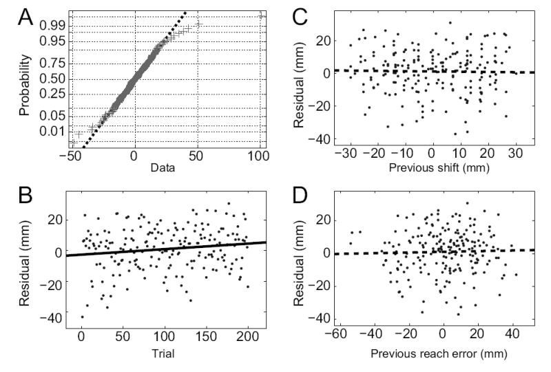
Examples of statistical analyses performed on the model prediction errors. A: Normal probability plot for the only residual component (x-component, Subject 8) that showed significant deviations from normality (N=199, Lilliefors test, p = 0.04). Data-points are represented by crosses; Gaussian data fall on a straight line (best fit line displayed as dashed line). Without the single large outlier (top-right of graph), the deviation from the Gaussian distribution is not significant (p > 0.2). B: Example of significant non-stationarity (linear regression, F-test, p = 0.036) in the model-fit residual (y-component, Subject 1). C,D: Example plots of model-fit residual (y-component, Subject 1) vs. visual shift on the prior trial (C) or reach error on the prior trial (D). Linear regression shows no significant effect in either plot (F-test, p = 0.79 and p = 0.69) and no clear non-linear relationships are discernible.
Non-stationarity
If the true learning dynamics were non-stationary, then we would expect our stationary LDS models to fit better at some times during the experiment and worse at other times. Therefore, we plotted the residuals as a function of trial number, and looked for changes across trials. Out of 20 such plots, three showed a significant linear dependence of residual on trial number (linear regression, F-test, α = 0.05). An example of a significant effect is shown in Fig. 10B. While these effects were observed slightly more often than expected by chance (3/20 = 15%), the significant comparisons had weak correlations (r2 < 0.034) and were never found in both residual components of the same subject. Across subjects there are no discernible non-linear trends in the residuals, nor were there any apparent changes in the variance of the residuals across trials.
Non-linearity
If the true learning dynamics were nonlinear, then the LDS prediction errors would contain a component that was a deterministic function of one of the key variables driving learning. Therefore, we examined whether the model-fit residuals across trials covary with either of the key variables that influence the dynamics of learning, the visual shift and the reach error from the previous trial. Not one of the 20 comparisons showed a significant linear dependence of residual on either the previous visual shift or the previous reach error (linear regression, F-test, α = 0.05). Representative examples are shown in Figs. 10C and 10D. As in these examples, there were also no discernible non-linear relationships between the residuals and the task variables.
References
- Anderson BDO, Moore JB. Optimal Filtering. Prentice-Hall; Englewood Cliffs, N.J: 1979. [Google Scholar]
- Atkeson CG, Hollerbach JM. Kinematic features of unrestrained vertical arm movements. J Neurosci. 1985;5(9):2318–30. doi: 10.1523/JNEUROSCI.05-09-02318.1985. [DOI] [PMC free article] [PubMed] [Google Scholar]
- Baddeley RJ, Ingram HA, Miall RC. System identification applied to a visuomotor task: Near-optimal human performance in a noisy changing task. J Neurosci. 2003;23(7):3066–3075. doi: 10.1523/JNEUROSCI.23-07-03066.2003. [DOI] [PMC free article] [PubMed] [Google Scholar]
- Baizer JS, Glickstein M. Proceedings: Role of cerebellum in prism adaptation. J Physiol. 1974;236(1):34P–35P. [PubMed] [Google Scholar]
- Baizer JS, Kralj-Hans I, Glickstein M. Cerebellar lesions and prism adaptation in macaque monkeys. J Neurophysiol. 1999;81(4):1960–1965. doi: 10.1152/jn.1999.81.4.1960. [DOI] [PubMed] [Google Scholar]
- Bedford FL. Perceptual and cognitive spatial learning. J Exp Psychol. 1993;19(3):517–530. doi: 10.1037//0096-1523.19.3.517. [DOI] [PubMed] [Google Scholar]
- Cheng S, Sabes PN. Modeling sensorimotor adaptation as linear dynamical system. Neural Comput. 2006;18(4):760–793. doi: 10.1162/089976606775774651. [DOI] [PMC free article] [PubMed] [Google Scholar]
- Choe CS, Welch RB. Variables affecting the intermanual transfer and decay of prism adaptation. J Exp Psychol. 1974;102(6):1076–1084. doi: 10.1037/h0036325. [DOI] [PubMed] [Google Scholar]
- Clower DM, Hoffman JM, Votaw JR, Faber TL, Woods RP, Alexander GE. Role of posterior parietal cortex in the recalibration of visually guided reaching. Nature. 1996;383:618–621. doi: 10.1038/383618a0. [DOI] [PubMed] [Google Scholar]
- Davies N, Newbold P. Some power studies of a portmanteau test of time-series model specification. Biometrika. 1979;66(1):153–155. [Google Scholar]
- Donchin O, Francis JT, Shadmehr R. Quantifying Generalization from Trial-by-Trial Behavior of Adaptive Systems that Learn with Basis Functions: Theory and Experiments in Human Motor Control. J Neurosci. 2003;23(27):9032–9045. doi: 10.1523/JNEUROSCI.23-27-09032.2003. [DOI] [PMC free article] [PubMed] [Google Scholar]
- Ghahramani Z, Hinton GE. Technical Report CRG-TR-96-2. University of Toronto, Department of Computer Science; 6 King’s College Road, Toronto, Canada M5S 1A4: 1996. Parameter estimation for linear dynamical systems. [Google Scholar]
- Gordon J, Ghilardi M, Ghez C. Accuracy of planar reaching movements. I. Independence of direction and extent variability. Exp Brain Res. 1994;99(1):97–111. doi: 10.1007/BF00241415. [DOI] [PubMed] [Google Scholar]
- Harris CM, Wolpert DM. Signal-dependent noise determines motor planning. Nature. 1998;394(6695):780–784. doi: 10.1038/29528. [DOI] [PubMed] [Google Scholar]
- Harris CS. Adaptation to displaced vision: visual, motor, or proprioceptive change? Science. 1963;140:812–813. doi: 10.1126/science.140.3568.812. [DOI] [PubMed] [Google Scholar]
- Hatada Y, Rossetti Y, Miall RC. Long-lasting aftereffect of a single prism adaptation: shifts in vision and proprioception are independent. Exp Brain Res. 2006;173(3):415–424. doi: 10.1007/s00221-006-0381-2. [DOI] [PubMed] [Google Scholar]
- Hay JC, Pick HL. Visual and proprioceptive adaptation to optical displacement of the visual stimulus. J Exp Psychol. 1966;71(1):150–158. doi: 10.1037/h0022611. [DOI] [PubMed] [Google Scholar]
- Held R, Gottlieb N. Technique for studying adaptation to disarranged hand-eye coordination. Percept Mot Skills. 1958;8:83–86. [Google Scholar]
- Hosking JRM. The multivariate portmanteau statistic. J Am Stat Assoc. 1980;75(371):602–608. [Google Scholar]
- Hua SE, Houk JC. Cerebellar guidance of premotor network development and sensorimotor learning. Learn Mem. 1997;4(1):63–76. doi: 10.1101/lm.4.1.63. [DOI] [PubMed] [Google Scholar]
- Kurata K, Hoshi E. Reacquisition deficits in prism adaptation after muscimol microinjection into the ventral premotor cortex of monkeys. J Neurophysiol. 1999;81(4):1927–1938. doi: 10.1152/jn.1999.81.4.1927. [DOI] [PubMed] [Google Scholar]
- Ljung L. System Identification: Theory for the User. 2 Prentice Hall PTR; Upper Saddle River, NJ 07458: 1999. [Google Scholar]
- Magescas F, Prablanc C. Automatic drive of limb motor plasticity. J Cogn Neurosci. 2006;18(1):75–83. doi: 10.1162/089892906775250058. [DOI] [PubMed] [Google Scholar]
- Messier J, Kalaska JF. Differential effect of task conditions on errors of direction and extent of reaching movement. Exp Brain Res. 1990;125(2):139–52. doi: 10.1007/pl00005716. [DOI] [PubMed] [Google Scholar]
- Miles F, Fuller J. Adaptive plasticity in the vestibulo-ocular responses of the rhesus monkey. Brain Res. 1974;80(3):512–516. doi: 10.1016/0006-8993(74)91035-x. [DOI] [PubMed] [Google Scholar]
- Nemenman I. Fluctuation-dissipation theorem and models of learning. Neural Comput. 2005;17(9):2006–2033. doi: 10.1162/0899766054322982. [DOI] [PubMed] [Google Scholar]
- Optican LM, Robinson DA. Cerebellar-dependent adaptive control of primate saccadic system. J Neurophysiol. 1980;44(6):1058–1076. doi: 10.1152/jn.1980.44.6.1058. [DOI] [PubMed] [Google Scholar]
- Osborne LC, Lisberger SG, Bialek W. A sensory source for motor variation. Nature. 2005;437(7057):412–416. doi: 10.1038/nature03961. [DOI] [PMC free article] [PubMed] [Google Scholar]
- Redding G, Wallace B. Adaptive mechanisms in perceptual-motor coordination: components of prism adaptation. J Mot Behav. 1988;20(3):242–254. doi: 10.1080/00222895.1988.10735444. [DOI] [PubMed] [Google Scholar]
- Redding GM, Rossetti Y, Wallace B. Applications of prism adaptation: a tutorial in theory and method. Neurosci Biobehav Rev. 2005;29(3):431–444. doi: 10.1016/j.neubiorev.2004.12.004. [DOI] [PubMed] [Google Scholar]
- Salinas E, Abbott LF. Transfer of coded information from sensory to motor networks. J Neurosci. 1995;15(10):6461–6474. doi: 10.1523/JNEUROSCI.15-10-06461.1995. [DOI] [PMC free article] [PubMed] [Google Scholar]
- Scheidt R, Dingwell J, Mussa-Ivaldi F. Learning to move amid uncertainty. J Neurophysiol. 2001;86(2):971–985. doi: 10.1152/jn.2001.86.2.971. [DOI] [PubMed] [Google Scholar]
- Shumway RH, Stoffer DS. An approach to time series smoothing and forecasting using the EM algorithm. J Time Series Analysis. 1982;3(4):253–264. [Google Scholar]
- Smith MA, Ghazizadeh A, Shadmehr R. Interacting adaptive processes with different timescales underlie short-term motor learning. PLoS Biol. 2006;4(6):e179. doi: 10.1371/journal.pbio.0040179. [DOI] [PMC free article] [PubMed] [Google Scholar]
- Sober S, Sabes P. Flexible strategies for sensory integration during motor planning. Nat Neurosci. 2005;8(4):490–497. doi: 10.1038/nn1427. [DOI] [PMC free article] [PubMed] [Google Scholar]
- Stuart A, Ord JK. Kendall’s advanced theory of statistics. 5 Oxford University Press; New York: 1987. [Google Scholar]
- Taub E, Goldberg L. Prism adaptation: control of intermanual transfer by distribution of practice. Science. 1973;180(87):755–7. doi: 10.1126/science.180.4087.755. [DOI] [PubMed] [Google Scholar]
- Thoroughman KA, Shadmehr R. Learning of action through adaptive combination of motor primitives. Nature. 2000;407:742–747. doi: 10.1038/35037588. [DOI] [PMC free article] [PubMed] [Google Scholar]
- van Beers R, Sittig A, Denier van der Gon J. The precision of proprioceptive position sense. Exp Brain Res. 1998;122(4):367–377. doi: 10.1007/s002210050525. [DOI] [PubMed] [Google Scholar]
- Welch RB. Perceptual Modification: Adapting to Altered Sensory Environments. Academic Press, Inc; New York: 1978. [Google Scholar]
- Welch RB, Choe CS, Heinrich DR. Evidence for a three-component model of prism adaptation. J Exp Psychol. 1974;103(4):700–705. doi: 10.1037/h0037152. [DOI] [PubMed] [Google Scholar]