Adaptive Border Marching Algorithm: Automatic Lung Segmentation on Chest CT Images

Abstract

Segmentation of the lungs in chest computed tomography (CT) is often performed as a preprocessing step in lung imaging. This task is complicated especially in presence of disease. This paper presents a lung segmentation algorithm called Adaptive Border Marching (ABM). Its novelty lies in the fact that it smoothes the lung border in a geometric way and can be used to reliably include juxtapleural nodules while minimizing oversegmentation of adjacent regions such as the abdomen and mediastinum. Our experiments using 20 datasets demonstrate that this computational geometry algorithm can re-include all juxtapleural nodules and achieve an average oversegmentation ratio of 0.43% and an average undersegmentation ratio of 1.63% relative to an expert determined reference standard. The segmentation time of a typical case is under 1 minute on a typical PC. As compared to other available methods, ABM is more robust, more efficient and more straightforward to implement, and once the chest CT images are input, there is no further interaction needed from users. The clinical impact of this method is in potentially avoiding false negative CAD findings due to juxtapleural nodules and improving volumetry and doubling time accuracy.

I. INTRODUCTION

X-ray computed tomography (CT) is widely recognized as one of the most sensitive diagnostic imaging modalities for lung analysis such as lung nodule detection [1–3] and airway analysis [4]. Whole lung segmentation is often used prior to these analyses to reduce computation and limit extraneous results. Although threshold-based region-filling strategies [5–8] can be used to extract the lung parenchyma efficiently, they often incorrectly exclude some very important regions, such as juxtapleural nodules, from the segmentation because they are contiguous with the chest wall and have a similar density. Since no other clinically used imaging modalities and/or contrast agents can create reliable contrast between the soft tissues of juxtapleural nodules/hilum and the soft tissues of the chest wall, this problem must be solved by image analysis algorithms. Ameliorating the under-segmentation of juxtapleural lung nodules is important for lung nodule detection and characterization. Unfortunately, designing an efficient and robust segmentation algorithm is difficult because of the highly varied properties of juxtapleural nodules such as shape, size, intensity, and location. Additionally, a good solution should not only include juxtapleural nodules properly, but also minimize undersegmentation of the lung and oversegmentation of non-lung structures. Small inaccuracies in inclusion of juxtapleural nodules could lead to inaccurate volumetric measurement and estimation of malignancy [9] and doubling times [10–13].

Many methods [14–17] have been proposed to segment the lung automatically in volumetric CT images and only some explicitly handle juxtapleural nodules but without any evaluation. In earlier research [18, 19], manual editing-approaches were used to ameliorate the undersegmentation of juxtapleural nodules, but this is extremely laborious and prone to intra- and inter-observer variability. In [1, 6], a rolling ball filter was applied to the lung segmentation border obtained from a threshold-based method for juxtapleural nodule correction. As pointed out in [20], it is difficult to find a properly-sized rolling ball a priori that works well for all juxtapleural nodules. If the radius is too small, juxtapleural nodules will be undersegmented. If the radius is too large, computational cost increases substantially, and oversegmentation and distortion of local shape occurs, particularly near the hilum. Kim et al. [20] used a contour-following method that tracked the segmented lung boundaries to detect a seed area with texture features of a true juxtapleural nodule. However, texture features alone do not define juxtapleural nodules, which can be defined more accurately by their position and geometric features. Goo et al. [21] proposed that the contour indentations caused by juxtapleural nodules could be bridged and filled but provided no algorithmic details. Another solution was proposed to include juxtapleural nodules by searching for circular or semi-circular structures along the lung wall [22]. In practice, the shapes of juxtapleural nodules vary greatly from round and oval to cone, triangular, and flat [23] and, therefore, this method may fail for juxtapleural nodules with tubular or cone-like shapes. In [8, 24–26], a sequence of erosion and dilation operations was used to smooth the lung border as an alternative to the rolling ball method. The difference between the erosion/dilation operations and the rolling ball method lies in the design of a structuring element. They still face the same issues as the rolling ball method. In addition, some methods [27, 28] use curvature to correct the lung border with juxtapleural nodules. The motivation for the curvature-based method arises from the observation that a rapid change in curvature usually indicates a nodule, large vessel or bronchus. Thus, by comparing the curvature at points on the lung border, the regions with juxtapleural nodules can be found and re-included by inserting a border segment. However, curvature is not a robust criterion since local, small perturbations in shape might cause a rapid change of curvature and the normal lung base and apices have high curvature. Also, a single global curvature threshold may not exist that works for all cases. Gurcan et al. [29] designed a method for indentation detection that computes the ratio between the geodesic distance of two points on the border and the Euclidean distance of the line segment formed by the same two points. If the ratio is larger than a predefined threshold, then the lung border between the two points is replaced by the straight line through the two points.

In this paper, a fully automatic lung segmentation algorithm called Adaptive Border Marching (ABM) is introduced to segment the lung and correct the segmentation defects caused by juxtapleural nodules while minimizing undersegmentation and oversegmentation relative to the true lung border. The primary emphasis and distinguishing characteristic of the proposed method is on robustly correcting missed juxtapleural nodules. To evaluate the performance of this algorithm, experiments were conducted to evaluate: (1) the per-nodule sensitivity of the re-inclusion of juxtapleural nodules; and (2) the per-voxel undersegmentation and oversegmentation rates. We present examples as well as an analytical comparison between the rolling ball approach and our algorithm that demonstrate the advantages of our method.

II. MATERIALS AND METHODS

A. Overview of Adaptive Border Marching (ABM)

Fig. 1 illustrates the basic steps of our method. The preprocessing stage takes a 3D chest CT dataset as input and, in three steps [Fig. 1 (a)~(c)], converts the dataset to a form where the lung border can be easily extracted in vector form as the input for our proposed ABM algorithm. Because this stage can be done with well established techniques, the three steps involved will be explained briefly. The second stage is the main contribution of this paper. It also contains three steps [Fig. 1 (d)~(f)] and aims to correct the defects caused by the exclusion of juxtapleural nodules. Below we explain the proposed method in detail.

Fig. 1.

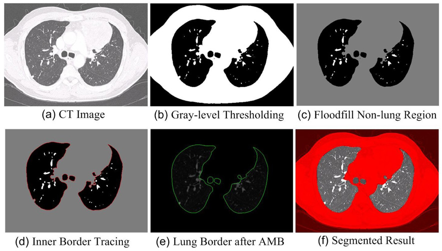
The basic steps of our lung segmentation scheme (a)~(f).

B. Preprocessing

The preprocessing stage contains three steps: 1) Gaussian Smoothing of the 3D CT Images [Fig.1 (a)]: Gaussian smoothing is used to remove the tiny isolated pockets of air between the patient and the CT bed in the images that lead to many small contours after the lung border tracing step that will be introduced below. These small contours will be incorrectly regarded as lung border. In our implementation, the CT images are convolved with a 3D Gaussian kernel that has a standard deviation of 1.0 mm. 2) Gray-level Thresholding [Fig.1 (b)]: In CT image data, the intensity of lung tissue is generally in the range of −400 HU to −600 HU, while the chest wall, blood, and bone is generally above −100 HU [30]. In our method, −500 HU is selected as the threshold to obtain the lung regions. 3) Floodfill Non-lung Region [Fig.1 (c)]: To remove non-lung regions left after thresholding, 2D flooding operation is performed slice by slice using the pixels along the image borders as flooding seeds. 2D flooding is used instead of 3D so that vessels that weave in and out of plane are included in the segmentation as intended.

C. Lung Region Computation

1) Lung Border Tracking [Fig.1 (d)]

After preprocessing, a well-known inner border tracing algorithm is used to compute the lung border by tracing the lung region [31]. The border of the lung region in each slice is traced in a sequence of pixels, thus forming a collection of directed closed contours:

$$\mathit{\text{Lungborder}}=\left\{L_i|(p_1,p_2,\dots ,p_{n_i}),i\in \left[1,m\right]\right\}$$ (1)

where m is the number of the directed loops forming the lung border, l_i is the i^th direction loop of the lung border, p_x is the pixel of the lung border.

2) Adaptive Border Marching (ABM) [Fig.1 (e)]

For didactic purposes, we present here a non-adaptive version of border marching even though it is not used in the final algorithm but is the basis of the ABM algorithm. After that, we will explain the ABM algorithm.

a) Non-adaptive Border Marching

To bridge the local concavities formed by improperly excluded juxtapleural nodules, our algorithm marches along the border with a marching step length and finds all of the convex tracks. The convex track is defined as the line segment connecting the starting point and the rightmost or leftmost point within the marching step. When the marching direction is clockwise, the leftmost line within the marching step is defined as the convex track; when the marching direction is counter-clockwise, the rightmost line within the marching step is defined as the convex track. For simplicity, counter-clockwise is used as the marching direction in this paper.

Whether a point is located on the right or left of a directed line can be simply determined by the right-hand rule, which checks the orientation of the rotation angle between two vectors, i.e., the vector of this line and the vector formed by the point and the starting point of the line. In our method, we need to find the right-most point within the marching step that is often formed by multiple points. To do this, the basic steps involved are: (1) Choose the first two points within the marching step as the directed reference line and the direction is along the marching direction [Fig. 2 (a)]. (2) Use the right-hand rule to check the relationship between the remaining points within the marching step and the directed reference line. If the point is located on the right side of the directed reference line, then a new directed reference line is formed by connecting the first point and this point [Fig. 2(b)]. (3) Repeat Step (2) until all the points within the marching step length are traversed. The point forming the end point of the final reference line is regarded as the rightmost point [Fig. 2(d)].

Fig. 2.

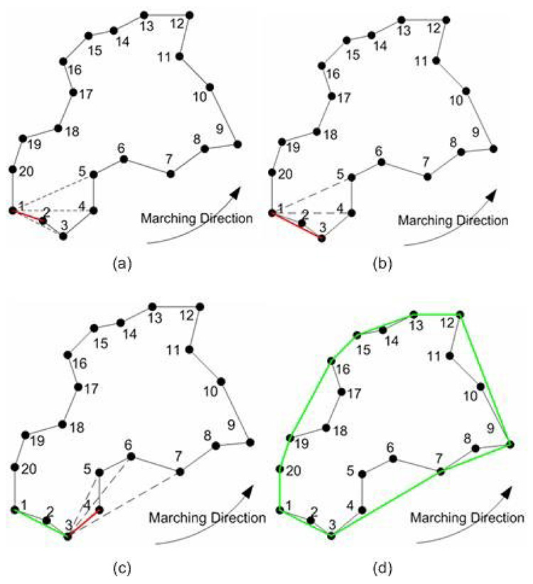
Basic steps for marching border algorithm and the marching step in this simplified example is every five points: (a) point 1 is selected as the starting point and p₁p₂ is selected as the directed reference line marked in red; (b) the directed reference line p₁p₂ is replaced with p₁p₃ because point 3 is found to be on the right side of the last directed reference line p₁p₂; (c) because the remaining points within the marching step length are all on the left side of the reference line, the directed reference line becomes a convex track in green and another round of marching operation starts again where the starting point is replaced with point 3; and (d) the border in green is the final result after repeating (a)~(c).

When the above algorithm is applied to CT lung images, example output is shown in Fig. 3, where the marching step length is measured in pixels along the lung border. The juxtapleural nodule can be properly included if the marching step length is larger than a certain value that varies according to the size of the juxtapleural nodule. However, when the marching step is too large, significant amounts of non-lung tissue are included, too, particularly in concave regions such as the mediastinal surface of the lung [Fig. 3(c)]. Also, the larger the marching step is, the more significant the over-segmentation will become. On the contrary, if the marching step is small [Fig. 3(a)~(b)], the juxtapleural nodules will not be fully included. Our experience with non-adaptive border marching is that even a judicious choice of static marching step length that effectively includes juxtapleural nodules will lead to erroneous inclusion of narrow slivers of chest wall on concave surfaces of the lung.

Fig. 3.

Segmented lungs using the non-adaptive approach with different marching steps (MB).

b) Adaptive Border Marching

To overcome the aforementioned oversegmentation limitation [Fig. 4(a)], we have developed a solution using an adaptive marching step length. The over-segmentation issue is modeled with two parameters [Fig. 4(b)]. One parameter is W, the Euclidean distance between two consecutive points after the marching operation, and the other is H_max, the maximum height perpendicular to this connecting line segment. To locate oversegmented regions, the step size is reduced adaptively when this ratio, λ, falls below a threshold value λ_o satisfying the “adaptive condition”:

$$\lambda =\frac{H_{\text{max}}}{W}$$ (2)

Given a local region, if λ is smaller than a threshold λ_o , then the marching step for this region is decreased by a scaling factor δ ∈ [0,1] (0.9 in our implementation), and the smoothing operation is executed again until λ within the new marching step is smaller than λ_o. The threshold λ_o can be optimized to the specific appearance of juxtapleural nodules.

Fig. 4.

Identification of over-segmentation errors: (a) an example with oversegmentation; and (b) a generic model for characterizing oversegmentation.

3) Lung Region Computation [Fig.1 (f)]

After the Adaptive Border Marching algorithm is carried out upon the lung contours, a new set of contours is formed and they can be regarded a set of closed polygons. By simply checking out all pixels within the polygons, we will find out the lung region. Now, by stacking the segmented slices, we can get the final 3D lung region.

E. Testing Datasets and Evaluation Methods

1) Testing Datasets

Twenty CT datasets were used for the analysis and experiments. Twenty-one consecutive outpatients scanned for suspicion of pulmonary nodules were scanned (age 15–91, mean 64; 16 male/5 female). One patient with active diffuse mycobacterial infection was excluded because of the presence of large areas of heterogeneous parenchymal consolidation and mucus plugs, which hindered the confident identification of pulmonary nodules in the reference reading. Please refer to [32] for a full description of these datasets. All these datasets were acquired without an intravenous contrast agent, from the lung apices through the upper abdomen, by using a four–detector row CT scanner (Volume Zoom; Siemens Medical Systems, Erlangen, Germany). Detector configuration was set to 4×1-mm section thickness, pitch of 1.5–1.75, gantry rotation time of 0.5 second, tube potential of 120 kVp, and tube current of 200–300 mA. The data were reconstructed into 1.25-mm-thick sections at 0.6-mm intervals by using a high resolution reconstruction kernel. The number of sections reconstructed per patient ranged from 431 to 664 (mean, 540). In total, 327 lung nodules (maximum diameter range: 1.5–18 mm; mean 4.1 mm) were determined by a consensus panel of three radiologists using 2D+3D image review, among which 67 were juxtapleural nodules. The lung contours were manually segmented by one radiologist and the results were used as the reference standard. To aid this manual segmentation, we developed a tool that allows the radiologist to threshold the images and then manually place splines to correct all areas of inaccuracy.

2) Evaluation Methods

To evaluate the segmentation performance, we measured three error metrics: re-inclusion ratio of juxtapleural nodules (per-nodule sensitivity), and the per-voxel oversegmentation and undersegmentation rates. Oversegmentation is defined as the lung volume that is regarded as lung tissue in our segmentation method while not in the reference standard, and the undersegmentation is vice versa. They were both compared with the total lung volume in the reference standard. Whether a juxtapleural nodule was correctly included or not was determined by a radiologist to see whether there are obvious defects in the segmentation due to juxtapleural nodules. We use the cumulative distribution to demonstrate the fitting between the lung surfaces obtained by the Adaptive Border Marching algorithm and the lung surfaces in the reference standard. The cumulative distance distribution is formed by calculating the shortest distance between a point on the lung surfaces obtained by the Adaptive Border Marching algorithm and the lung surfaces in the reference standard.

III. RESULTS

A. Non-adaptive Approach vs. Adaptive Approach

As compared to the adaptive approach, the non-adaptive method will usually introduce more slivers of oversegmentation due to the constant marching step length. To examine the effects of the oversegmentation introduced by the two approaches, we examined a set of 50 circles with different radii, ranging from 5 to 500 in pixels, as input to the two methods. These cause concavities of the black regions (lungs) that are similar to those caused by the mediastinum and liver. To demonstrate their difference clearly, a set of circles [Fig. 5] are used to simulate the concave regions of the lungs. A sequence of circles of decreasing radius was selected to represent the range of curvatures that would be encountered in the lungs and demonstrate the success of the adaptive approach at all these curvatures. For the non-adaptive method, oversegmentation is more significant as the radius decreases. In contrast, the adaptive approach shows virtually no oversegmentation of the concave regions at any of the test radii.

Fig. 5.

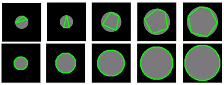
Examples obtained by the non-adaptive approach (top row) and the adaptive approach (bottom row). In both examples radius varies from 20 to 60 pixels. For the non-adaptive approach, the marching step is set as 50 pixels and does not change in the marching process. For the adaptive approach, the initial marching step is set as 50 pixels and will change adaptively in the marching process.

B. Adaptive Border Marching Accuracy

By testing against the 20 datasets, our experiments show that all 67 juxtapleural nodules were correctly re-included and added to the segmentation for a per-nodule sensitivity of 100%. An example of the comparison between the original lung boundary and the new lung boundary obtained by the Adaptive Border Marching algorithm is shown in Fig. 6.

Fig. 6.

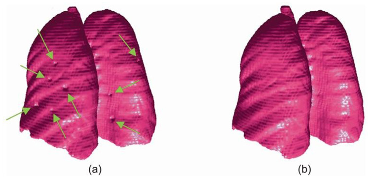
Lung segmentation results: (a) original boundary with juxtapleural nodules indicted by arrows; and (b) smoothed boundary obtained by the Adaptive Border Marching algorithm. The lung 3D models are created by marching cubes algorithm and formed by triangle mesh without any simplification or smoothing.

The oversegmentation and undersegmentation ratios for the 20 datasets are shown in Fig. 7. The average oversegmentation volume error per case is 0.43% of the true volume, while the average undersegmentation is 1.63%. It can be seen from Fig. 7 that the undersegmentation ratios of case 3 and case 15 are significantly larger than the other cases. We found that these large undersegmentation ratios are caused by a large hilar region, and consolidation, respectively, as demonstrated by Fig. 8.

Fig. 7.

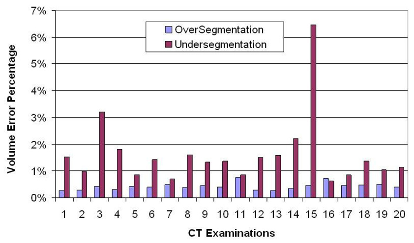
The volume-based segmentation error of the algorithm calculated as a percentage of the manual reference standard computed for both over- and under-segmentation. Mean errors are 0.43% and 1.63%, respectively.

Fig. 8.

Two cases (one typical, one difficult) with large undersegmentation ratios: (a) and (b) are images from case 3, (c) and (d) are images from case 15, (a) and (c) are reference standard, and (b) and (d) are the segmentation results by the border marching algorithms.

The cumulative error distance distribution is shown in Fig. 9. 94.2%, 98.9%, 95.4% of the lung surfaces obtained by our algorithm were within 2 mm of the reference standard, respectively, for undersegmentation, oversegmentation and the plus of over- and under-segmentation. The largest error for undersegmentation is 30 mm, while the largest error for oversegmentation is 6 mm. The error bars in Fig. 9 indicate the standard deviation of the cumulative percentage at the corresponding distance. Note that the high percentage of errors within a voxel or two is due to the excellent match of high contrast edges where no juxtapleural nodules or hilum are present to cause disagreement. The average number of points consisting of lung surfaces per case of the 20 cases is approximately 500,000. In addition, the computation time of our method is under 1 minute per case on average using a typical PC computer (AMD Athlon™ 64 X2 Dual, 2.11GHz, 2GB RAM), which is more computationally efficient than the rolling ball method.

Fig. 9.

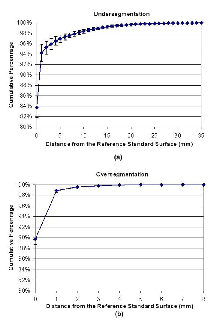
Cumulative distribution of point-wise shortest distance error to the gold standard surface obtained by the Adaptive Border Marching algorithm and the lung surfaces of the gold standard: (a) undersegmentation and (b) oversegmentation.

IV. DISCUSSION

A. Parameter Analysis of the Adaptive Border Marching Algorithm

In the Adaptive Border Marching algorithm, there are three parameters: the initial marching step length, the adaptive threshold λ_o, and the scale factor δ when the adaptive condition is met. The marching step length can be simply assigned an arbitrary value that is larger than the circumference of any juxtapleural nodule and the adaptive algorithm will find the appropriate step adaptively. In Fig. 10, an example is shown to demonstrate the effect of the initial marching step length upon the final result. For interactive applications, the marching step length could be used to control the fit between the smoothed result and the original border. The smaller the step length is, the more precise the smoothed result fits the original border.

Fig. 10.

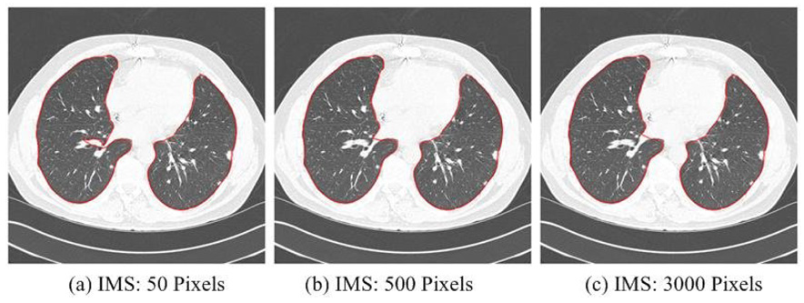
Example of segmented results using different initial marching steps (IMS) and the adaptive approach, demonstrating the robustness to IMSL over nearly two orders of magnitude change.

The scale factor δ determines the rate of change of the marching step length during the adaptive process. A smaller δ will lead to a rapid change of marching step, while a larger δ will lead to a slow change of the marching step. When the marching step is changed too quickly, the optimum marching step might be skipped, thus leading to an undesirable result. Ideally, a value as close to 1 should be chosen such that undue computational burden is avoided. In our case, we found a value of 0.9 to be quite reasonable both in terms of accuracy and computational efficiency.

The purpose of the adaptive threshold λ_o is to determine a proper marching step according to the shape of the local region. Although it is intuitive to use curvature to describe the shape change, we found this to be inherently a localized measurement very susceptible to noise. Instead, we intend to use a more global measure of these shape anomalies that is less susceptible to small perturbations in contour. For the sake of simplicity, we examine the λ measurement on an idealized hemicircle shape perturbation with radius of curvature R as shown in Fig. 11. If the width W is changed by the adaptive algorithm, the maximum height H_max also changes according to:

$$\lambda =\frac{H_{\text{max}}}{W}=\frac{R-\sqrt{R^2-\frac{1}{4}{W}^2}}{W}$$ (3)

Fig. 11.

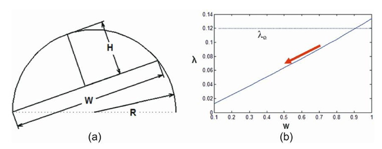
Changes in adaptive condition λ_o : (a) a hemicircle with a radius R; and (b) the plotted curve of the relationship between W and λ.

Note that for a simple object such as a hemicircle, λ is not scale-free (i.e., constant with respect to changing W and constant R) unlike curvature and in fact, varies approximately linearly. This interesting property is what gives this adaptive algorithm significant robustness by adaptively reducing W. If λ is above λ_o, the adaptive procedure does not proceed. However, if λ is below and W is reduced by the adaptive procedure, the gap between λ and λ_o will grow reducing the likelihood that the adaptive procedure stops prematurely due to naturally occurring variations in shape away from our idealized hemicircle. Thus, the adaptive nature of this algorithm encourages either complete re-inclusion of juxtapleural nodules (λ>λ_o) or a match to the threshold-based border when juxtapleural nodules are not present (λ <λ_o). This “all or nothing” characteristic yields excellent performance in fixing juxtapleural nodules without leaving “slivers”.

Due to the fact that the practical juxtapleural nodules are not exact hemicircles, the adaptive condition λ_o should be set a value less than 0.5 that actually indicates a perfect hemicircle. Meanwhile, λ_o should also be large enough to make sure that other concave regions will not be incorrectly regarded as juxtapleural region. In our implementation, λ_o is assigned with 0.33 yielding robust results.

B. Comparison with Rolling-ball Method

As a geometric approach, the method proposed in this paper has many valuable advantages over the often cited rolling-ball method for juxtapleural nodule segmentation. The reason that we conducted the comparison between the rolling ball method and our method analytically instead of running it directly on our own datasets is due to the fact that the parameter selection for rolling ball method is not straightforward and it is not a fair comparison to implement our own.

1) Computational Complexity Analysis

As a morphological operation, the rolling ball filter is a specific closing operation where the structural element is a circle. It consists of a dilation operation followed by an erosion operation. If the radius of a rolling ball is r pixels, the size of the structural element usually is (2×r+1)×(2×r+1) pixels and this is scanned across the image. The computational complexity of the basic algorithm will be O(r²×n²), where the size of the image is n×n. This is also the reason that many methods [33–35] have been proposed to increase the efficiency of morphological operations.

In the degenerate case when the initial marching step is larger than the length of the border, the non-Adaptive Border Marching method is equivalent to the well-known Jarvis March algorithm [31], which computes the global convex hull of an arbitrary set of points. Similar to the Jarvis March algorithm, the computational complexity of this proposed algorithm is O(kn), where n is the number of points forming the pre-smoothed border and k is the number of points formed the smoothed border. Obviously, in the worst cases the complexity is O(n²).

2) Effects of the Radius of the Rolling Ball

In [20], Kim et al. pointed out to the difficulty in selecting a fixed radius for the rolling ball method due to the size variance of juxtapleural nodules. In addition, there are other disadvantages of the rolling ball method. Small radius values will lead to an incomplete inclusion of juxtapleural nodules [Fig. 12(b)~(d)], which will cause incorrect volumetric measurement of the nodules. Although this issue can be partially alleviated when the radius is set large enough, it will lead to heavy computation and local shape changes [Fig. 12(e)]. In contrast, the adaptive border marching algorithm has no such limitations [Fig. 12(f)].

Fig. 12.

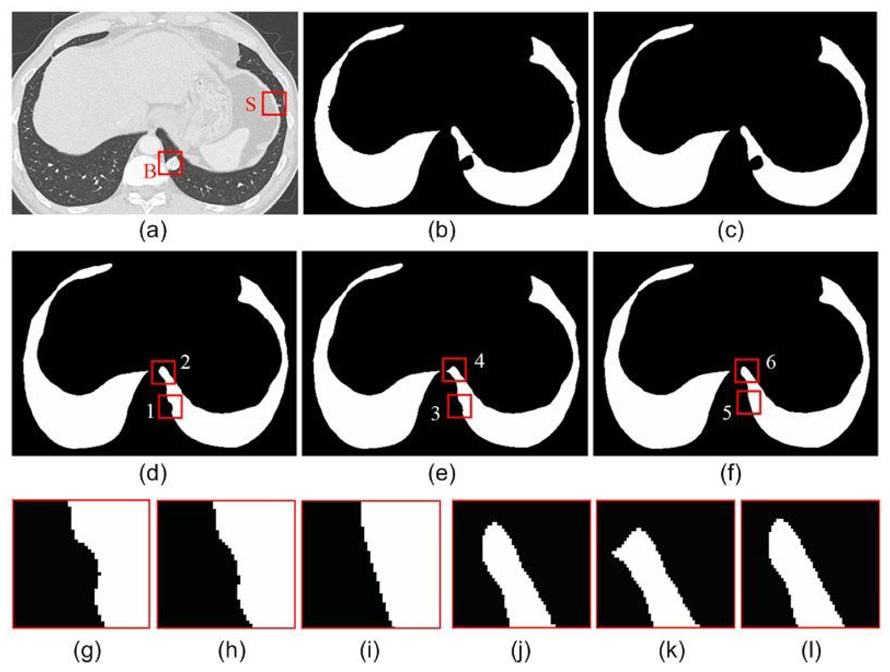
An example of the effect of the rolling ball radius on a juxtapleural nodule: (a) original CT image; (b) lung region obtained by thresholding; (c–e) the smoothed result obtained by the rolling ball method when the radius is set as 5 pixels, 10 pixels and 15 pixels, respectively; (f) the smoothed result obtained by our method; (g) the local enlargement indicated by “1” in (d); (h) the local enlargement indicated by “3” in (e); (i) the local enlargement indicated by “5” in (f); (j) the local enlargement indicated by “2” in (d); (k) the local enlargement indicated by “4” in (e); and (l) the local enlargement indicated by “6” in (f).

As compared the rolling ball method, which generalizes between 2D and 3D, our proposed algorithm is 2D because it requires a linear sequence (i.e., total ordering) of the set of contour points in order to march around the contour. However, there is no obvious way to create a linear sequence of the vertices of a 3D mesh and thus, there is no obvious order to march along a mesh.

C. Segmentation Evaluation Methodology

As compared to the numerous image segmentation methods proposed in the past decades, few approaches have ever been proposed in the field of medical image analysis to evaluate the segmentation algorithms in an intuitive and consistent way. Quantitative evaluation of a segmentation algorithm is crucial because it can not only provide a reliable basis for its clinical applications but also indicate its relative performance compared to other existing algorithms [36]. In his survey paper [37], Zhang classified the methods for segmentation evaluation into two categories: analytical methods [38–39] and empirical methods [40–41]. The analytical methods evaluate a segmentation algorithm by analyzing its properties, including its algorithm logic, complexity, requirement and efficiency, while the empirical methods judge a segmentation algorithm through experiments. Evaluating the performance of a lung segmentation approach is often difficult because the true lung boundary is unknown [40–42]. Often, the reference standard refers to the consensus of several experts. In this paper, our evaluations are performed from both perspectives proposed by Zhang [37]. The comparison between the rolling ball method and our method is mainly conducted analytically. Meanwhile, the reference standard was created manually under the guidance of one radiologist to avoid additional issues of combining multiple reference standards. Although the limited number radiologists involved in this manual segmentation might lead to bias, the difference between the lung boundaries obtained by our algorithm and the reference standard can reflect the errors of our segmentation method with respect to an expert. Given the reference standard, there still needs to be a distance metric that can measure the fit between the results obtained by the algorithm and the reference standard. Although many methods have been proposed to evaluate the performance of lung segmentation, such as pixel-wise XOR operations [41], Pratt Figure of merit [40] and partition distance [43], they do not offer both a local and global impression of the segmentation performance. In this paper, we demonstrate the segmentation performance using the error distance distribution [Fig. 9], which demonstrates not only an overview of the over- and under-segmentation, but also the whole statistical distribution of segmentation error distances.

V. CONCLUSION

As an important issue in pulmonary image analysis, segmentation has received much attention in the past and many methods have been proposed. In this paper, we have introduced a geometric algorithm that segments the lung using a novel Adaptive Border Marching algorithm. Unlike many previous pixel-based approaches, our method generalizes lung segmentation as a smoothing process of contours in continuous space. Fundamentally, this algorithm could be applied to any application where very specific localized indentations to otherwise smooth contours must be bridged. To demonstrate these advantages, an extensive analysis and experiments have been conducted and presented in this paper. As a computational geometry approach, our method has many advantages such as low computational cost, robust smoothing performance, easy implementation and no user interaction. The algorithm introduced in this paper is currently used as a precursor for lung nodule computer-aided detection.

Biographies

Justus Roos, MD, is now an assistant professor of radiology at Stanford University. His research interests focus around CT applications, with two main scholarly focuses on computer-aided detection of pulmonary nodules in chest CT scans and on cardiovascular CT visualization techniques. A major project has been to develop and validate new 3D post-processing methods of CT angiography data in patients with peripheral arterial occlusive disease.

Chin A Yi, MD, is now a postdoctoral scholar at Stanford University. She is affiliated with the Department of Radiology and Center for Imaging Science at Sunkyunkwan University School of Medicine, where she received her MD and residency training. Her research interests lie in pulmonary imaging, automated detection of lung nodules in CT data, and the impact investigation of CAD on the diagnostic performance of radiologists interpreting lung CT scans.

Geoffrey D. Rubin, M.D., is a Professor of Radiology and the Chief of the Cardiovascular Imaging Section at Stanford University, as well as a co-founder and the current medical Co-Director of Stanford's 3D Medical Imaging Laboratory. He received his MD from the University of California at San Diego and had his residency at Stanford University. His research interests focus on cardiovascular and pulmonary imaging.

Sandy Napel, Ph.D., is a Professor of Radiology, Professor of Medicine-Informatics (by courtesy) and Professor of Electrical Engineering (by courtesy) at Stanford University. He received his PhD in Electrical Engineering from Stanford University. He is currently Co-Directors of the Stanford Radiology 3D Medical Imaging Laboratory. His primary interests are in developing diagnostic and therapy-planning applications and strategies for the acquisition and visualization of multi-dimensional medical imaging data.

David Paik is an Assistant Professor in the Department of Radiology at Stanford University. He did his doctoral work in biomedical informatics at Stanford focusing on computer aided interpretation of medical images including anatomic modeling, visualization and computer aided diagnosis. He is currently working on several major projects that focus on bringing a quantitative and principled approach to medical image analysis with the ultimate goal of integrating image-derived information with other biomedical information sources.

Jiantao Pu is now a Research Assistant Professor at the University of Pittsburgh. His research interests include computer graphics, medical image processing, and human-computer interaction. He is a member of ACM Siggraph and the IEEE Engineering in Medicine and Biology Society. He received a PhD in computer science at Peking University. He worked as a postdoctoral research fellow at Purdue University and Stanford University respectively. Contact him at jip13@pitt.edu.