Testing for association on the X chromosome

Abstract

The problem of testing for genotype–phenotype association with loci on the X chromosome in mixed-sex samples has received surprisingly little attention. A simple test can be constructed by counting alleles, with males contributing a single allele and females 2. This approach does assume not only Hardy–Weinberg equilibrium in the population from which the study subjects are sampled but also, perhaps, an unrealistic alternative hypothesis. This paper proposes 1 and 2 degree-of-freedom tests for association which do not assume Hardy–Weinberg equilibrium and which treat males as homozygous females. The proposed method remains valid when phenotype varies between sexes, provided the allele frequency does not, and avoids the loss of power resulting from stratification by sex in such circumstances.

1. INTRODUCTION

Association between genetic markers and disease is most commonly demonstrated by case–control studies, in which the frequency distributions of genotype in cases and controls are compared. The most widely useful markers are single nucleotide polymorphisms (SNPs), which are chromosomal loci that have only 2 forms, or alleles. Since most human chromosomes occur in pairs (autosomes), there are 3 possible genotypes at such a locus. In the simplest case, the test for association commonly used is the conventional chi-squared 2 degree-of-freedom test for association in the 3×2 contingency table or the Cochran–Armitage 1 degree-of-freedom trend test. The former test makes no strong assumptions about the disease association, but the latter is sensitive to departures from the null in which the case–control ratio, reflecting risk in the underlying population, varies monotonically with genotype, ordered by the number of copies of a nominated allele (0, 1, or 2). An alternative method has been to carry out the 1 degree-of-freedom test for association in the 2×2 table which counts chromosomes, or alleles, in cases and controls. Unlike tests at the genotype level, this test assumes that the 2 chromosomes carried by each individual can be regarded as independently sampled from a population of chromosomes—the assumption of Hardy–Weinberg equilibrium (Sasieni, 1997). This test is closely related to the Cochran–Armitage test; both contrast the observed number of alleles in cases with the expected number under the null hypothesis, but these tests use difference variance estimates for this (O − E) statistic.

For SNPs on the X chromosome, females carry 2 copies but males carry only one copy. At first sight, it is obvious how the simple allele-counting method can be extended to this case: if the allele frequency in males and females can be assumed to be equal, we would count alleles in a 2×2 table and calculate a chi-squared test on 1 degree of freedom as before. However, 2 criticisms can be leveled at this approach; first, it assumes Hardy–Weinberg equilibrium in females, and second, males have only half the impact on the analysis as females. The latter problem reflects an implicit alternative hypothesis that the effect of 1 copy of a variant allele on phenotype is the same in males as in females. This may not be a realistic assumption.

These difficulties can be addressed in the usual method for analysis of case–control studies in epidemiology, that is, to treat the case–control status as the dependent variable in a logistic regression analysis (Prentice and Pyke, 1979), the genotype entering as a predictor variable. However, if the sex ratio differs between cases and controls, this necessitates inclusion of sex as a covariate—whether or not the allele frequency varies between sexes. This is equivalent to stratification of the analysis by sex and can lead to considerable loss of power. But when the allele frequency does not differ between sexes, stratification by sex, with its attendant loss in power, would seem unnecessary and undesirable.

The work described in this paper was motivated by a genome-wide association study in which a common control group was used for several groups of cases of different diseases. Inevitably, for some comparisons, the sex ratio differed markedly between cases and controls (Wellcome Trust Case Control Consortium, 2007). However, the problem is not unique to the case–control setting; it extends to any test for genotype–phenotype association for loci on the X chromosome—particularly when the distribution of phenotype varies substantially between the sexes.

In Section 2, the standard 1 and 2 degree-of-freedom tests for genotype–phenotype association for autosomal loci will be reviewed. The subsequent section discusses the modifications necessary for a locus on the X chromosome. Later sections discuss some extensions and alternative approaches.

2. AUTOSOMAL LOCI

In this section, the derivation of 1 and 2 degrees of freedom for association with autosomal loci will be briefly reviewed. These test statistics are based on genotype–phenotype covariances and can be derived as score tests in the context of generalized linear models (GLMs) (McCullagh and Nelder, 1989) which relate the expectation of the phenotype, transformed by a “link” function, to a linear model which may include “additive” and “dominance” components. The score statistics (Cox and Hinkley, 1974) are defined by first derivatives of the log-likelihood function with respect to additive and dominance effect parameters, evaluated under the null hypothesis, H₀, of no association. In the simplest case, only an additive effect is assumed; this will be discussed first.

2.1. Additive genetic model

For a general phenotype, the score statistic for testing for an additive effect of a diallelic locus on phenotype is the genotype–phenotype covariance

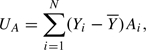where Y_i is the phenotype for subject i and A_i codes the corresponding genotype 1/1,1/2, and 2/2 to 0, 1, or 2, respectively. is the arithmetic mean of Y in the whole sample. (If there are additional covariates in the model and a link function other than the “canonical” link is used in the GLM, then additional weights are needed. This represents a minor extension and will not be discussed further here.)

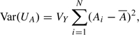
For reasons that will become clear later, although the test statistic has been introduced in terms of a model for the effect of genotype on phenotype, it is convenient, initially, to consider its distribution based on Pr(A_i|Y_i)(i = 1,…,N). Then, the statistic is asymptotically normally distributed under H₀ with 0 mean and variance

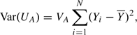where V_A is the variance of A_i (assumed constant for all i); this can be estimated by

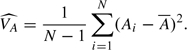Under H₀, the ratio is asymptotically distributed as chi-squared on 1 degree of freedom. A well-known special case of this test is the Cochran–Armitage test for a dichotomous phenotype or case–control data (Cochran, 1954), (Armitage, 1955), but it is equally applicable for a quantitative phenotype, even when the sample is selected by extremes of phenotype (Wallace and others, 2006). If Hardy–Weinberg equilibrium in the population can be assumed, the estimate of V_A may be replaced by

where P is the allele frequency, although this would not usually be recommended.

2.2. Dominance

The test above is locally most powerful against GLMs for genotype–phenotype association in which genotype enters as a linear term. Under such models, the heterozygous genotype, 1/2, falls midway between the 1/1 and 2/2 homozygous genotypes on the linear predictor scale. A broader class of alternatives is obtained by entering a “dominance” term in the linear model. A convenient way to do this is by an heterozygosity indicator, D say, taking the value 1 for heterozygotes and 0 for homozygotes. An additional score test statistic for the dominance effect is then

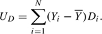The 2 degree-of-freedom test combines U_A and U_D. Under H₀, U_D also has 0 mean and

where V_D is the variance of each D_i and V_AD is the covariance between A_i and D_i. These can be estimated by

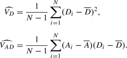(Again, alternative estimates can be used if one is prepared to assume Hardy–Weinberg equilibrium.) Then, writing

the statistic is asymptotically distributed under H₀ as chi-squared with 2 degrees of freedom. In the special case of a dichotomous phenotype, this test is identical to the conventional Pearsonian chi-squared test for association in the 3×2 contingency table.

3. THE X CHROMOSOME

Loci on the pseudo-autosomal part of the X chromosome can be treated in exactly the same way as autosomal loci, but others generally require different treatment. For these, males will only carry 1 copy, while, in females, most loci are subject to X inactivation (Chow and others, 2005), so that a female will have approximately half her cells with 1 copy active while the remainder of her cells have the other copy activated. Thus, in the absence of interaction with other loci or environmental factors, males should be equivalent to homozygous females in respect to such loci. This suggests that, for X loci in males, A_i should be coded 0 or 2, while D_i should be coded 0. This has several consequences, some of which require modifications to the theory outlined above.

1. If the allele frequency does not vary between sexes, the expectation of A is also equal (at 2P) for the 2 sexes. Thus, the expectation of U_A will remain at 0 under H₀ even when the phenotype, Y, is related to sex.

2. However, the variance of A differs between males and females. For example, under Hardy–Weinberg equilibrium, its variance is 2P(1 − P) in females and 4P(1 − P) in males. This means that, in general, an alternative variance estimate for U_A must be used.

3. Only females contribute to the dominance score, U_D. For notational simplicity, assume that subjects are arranged so that subjects 1,…,F are female and subjects (F + 1),…,N are male. Then,

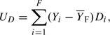where _F is the mean of Y “in females.”

A modified estimator for the variance–covariance matrix of U can now be derived. The variance–covariance matrix for A and D for females can be estimated by

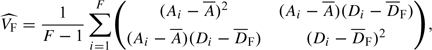where _F is the mean of D_i in females. (Since allele frequencies are assumed to be equal between males and females, may be calculated from the entire sample rather than from females alone.) In males, since there is only a single copy of the allele, this variance–covariance matrix can be estimated by

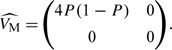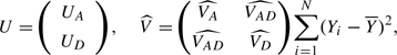
Again, P can be estimated in the entire sample, perhaps by allele counting or, alternatively, by /2. The variance–covariance matrix of the 2-vector of scores, U, is then estimated by

As before, the 2 degree-of-freedom chi-squared test is then given by , while the 1 degree-of-freedom test is given by . It should perhaps be emphasized that in the above expression for refers to the overall sample mean of the phenotype and not to the sex-specific means.

It has been stated above that the above modifications to U_D and to the estimator for the variance–covariance matrix are necessary “in general.” The exception is when sampling is carried out in such a way that the sample distributions of phenotype, Y (or at least their first 2 moments), are equal between males and females. Then, U_D, as defined for autosomal loci, will continue to have zero expectation under H₀, and the autosomal variance–covariance estimator will be unbiased (see Appendix A). This would occur, for example, in a case–control study in which cases and controls are frequency matched by sex.

4. STRATIFIED TESTS

Stratified score tests in which the alternative hypothesis is one of the equal effects of genotype on phenotype across strata are constructed by calculating the 2-vector of scores, U, and its estimated variance, , separately in each stratum. Both are then summed over strata. The final stratified chi-squared tests are then calculated in exactly the same way as before. This mirrors the classical Mantel–Haenszel generalizations of the standard 2×2 table association tests and the Mantel extension of the Cochran–Armitage test (Mantel and Haenszel, 1959), (Mantel, 1963). (It should be noted, however, that this assumes that the GLM which forms the alternative hypothesis uses a “canonical” link function; otherwise, the different stratum contributions would need to be weighted appropriately.)

The test outlined in Section 3 was derived under the assumption that the allele frequency does not vary with sex and, if this assumption cannot be made, it will be necessary to stratify by sex in the analysis. Note, however, that in the event of strong association between sex and phenotype, this will result in loss of power (perhaps considerable). An extreme example is provided by the unlikely case in which all the cases are female and all the controls male; stratification by sex leaves no information for testing association, whereas, if allele frequencies can be assumed to be equal between the sexes, valid test can be carried out as described in Section 3.

5. CONDITIONING ON GENOTYPE

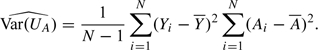
If only the 1 degree-of-freedom test were to be derived, a rather simpler derivation might have followed by taking the phenotype, Y, as the random response, deriving the distribution of U_A in sampling from Pr(Y_i|A_i)(i = 1,…,N). For an autosomal locus, this leads to precisely the same score test statistic, U_A, and

where V_Y is the variance of Y_i. Estimating V_Y by 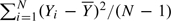then leads to an identical asymptotic test. Similarly, the 2 degree-of-freedom test can be derived in the same way.

It should be noted that a test based on U_A and the above expression for Var(U_A) remains valid in the presence of relationship between phenotype, Y, and sex, provided there is no relationship between genotype and sex. This follows from an argument which mirrors that presented in Appendix A but with the roles of genotype and phenotype reversed. However, in the presence of sex differences in the distribution of phenotype, differences in the mean of A between sexes lead to nonzero expectation for U_A under H₀, while a sex difference in the variance of A between sexes invalidates the above expression for Var(U_A). Either eventuality would render the standard test invalid. For autosomal loci, it will usually be safe to assume equality between the sexes for both the mean and the variance of A, but for loci on the X chromosome, while equality of the mean of A can usually be assumed, equality of the variances cannot.

Dependency of the variance of Y on sex can be allowed for by using separate estimates for males and females, in the same way as was used for the variance of A in the earlier derivation. Alternatively, a variance estimator in the spirit of the Huber–White “sandwich” estimator (Huber, 1967), (White, 1980) could be used. A valid Wald test for additive effect of a locus on the X chromosome could be carried out by simply regressing Y on A in a GLM and testing for a nonzero regression coefficient of A using a Huber–White estimate for the variance–covariance matrix of coefficients. The stratified version of the test would be obtained by additionally including the stratifying factor in the GLM. Generalized score tests which do not make the equal variance assumption have been discussed by Boos (1992).

At first, it seems natural to derive the 2 degree-of-freedom test in exactly the same way—by simply adding the heterozygosity indicators, D, into the model and testing for nonzero coefficients for both A and D. However, this is incorrect, since D is confounded with sex—males are always coded as homozygous, while females are only sometimes homozygous. Thus, when the phenotype varies with sex, this will generate a false dominance effect. Putting sex in the model corrects this but at the expense of power to detect the additive effect. There would seem to be no way to obtain the 2 degree-of-freedom test in 1 step by simple regression methods. It can, however, be done in 2 steps:

1. Calculate a 1 degree-of-freedom chi-squared test for additive effect, using a GLM in which neither dominance nor sex effects are included as predictors. To allow for the omission of sex from the model, Huber–White “robust” variance estimates must be used.

2. Calculate a 1 degree-of-freedom chi-squared test for dominance using a GLM which includes additive and dominance effects, together with sex. There is no need to use robust variance estimates at this stage.

Adding the 2 chi-squared tests yields a 2 degree-of-freedom test.

It would also be possible to test for a dominance effect by discarding males altogether. This would be less powerful since the additive effect would be less precisely estimated. However, this approach would be less reliant on the assumption that the effect of genotype in males mirrors that in homozygous females.

6. DISCUSSION

It has been argued that, when testing for genotype–phenotype association for loci on the X chromosome, males should be treated as homozygous females. If allele frequencies do not vary between the sexes, the additive genetic effect is not confounded with sex and there is no need to stratify by sex in the analysis. Indeed, to do so could seriously reduce power. However, if the first 2 moments of the distributions of phenotype are not equal in males and females, it becomes necessary to modify the variance calculations. In contrast, the dominance component of the genetic effect is, in general, confounded with sex, and testing for its presence requires allowance to be made for this fact.

This argument has been presented from the point of view of both probability models for genotype conditional on phenotype and for models for phenotype conditional on genotype. These are asymptotically (and sometimes algebraically) equivalent. However, the latter approach is more flexible in that it more naturally allows for the presence of further covariates.

FUNDING

The Wellcome Trust; the Juvenile Diabetes Research Foundation to D.C. Funding to pay the Open Access publication charges for this article was provide by The Wellcome Trust.

APPENDIX A

A.1. Ignoring sex in analyses of autosomes

The variance estimator for the score statistic U_A for autosomal loci is

When the variance of A differs between the sexes, it can be shown that

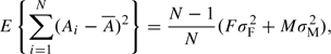where σ_F² and σ_M² are the variances of A in females and males, respectively, and F and M are the numbers of males and females in the sample. If the first and second sample moments of Y are equal for males and females, then

so that

This is the true variance of U_A when the variance of A differs between the sexes. Thus, when the first 2 sample moments of the phenotype Y do not differ between the sexes, the usual variance estimate will be unbiased even when the variance of A does differ between the sexes.

A similar argument shows that the usual variance estimator can be used when the distribution of phenotype varies between the sexes, provided that the first 2 moments of A do not vary between the sexes. This justifies ignoring sex (even when it has a strong effect) in analyses of autosomal loci.

References

- Armitage P. Test for linear trend in proportions and frequencies. Biometrics. 1955;11:375–386. [Google Scholar]
- Boos D. On generalized score tests. The American Statistician. 1992;4:327–333. [Google Scholar]
- Chow J, Yen Z, Ziesche S, Brown C. Silencing of the mammalian X chromosome. Annual Review of Genomics and Human Genetics. 2005;6:69–92. doi: 10.1146/annurev.genom.6.080604.162350. [DOI] [PubMed] [Google Scholar]
- Cochran W. Some methods of strengthening the common χ2 test. Biometrics. 1954;10:417–451. [Google Scholar]
- Cox D, Hinkley D. Theoretical Statistics. London: Chapman and Hall; 1974. [Google Scholar]
- Huber P. The behaviour of maximum likelihood estimates under non-standard conditions. In: Le Cam LM, Neyman J, editors. Proceedings of the Fifth Berkeley Symposium in Mathematical Statistics and Probability. Berkeley, CA: University of California Press; 1967. pp. 221–233. [Google Scholar]
- Mantel N. Chi-square tests with one degree of freedom: extension of the Mantel–Haenszel procedure. Journal of the American Statistical Association. 1963;58:690–700. [Google Scholar]
- Mantel N, Haenszel W. Statistical aspects of the analysis of data from retrospective studies of disease. Journal of the National Cancer Institute. 1959;22:719–748. [PubMed] [Google Scholar]
- McCullagh P, Nelder J. Generalized Linear Models (Second Edition), Monographs on Statistics and Applied Probability. London: Chapman and Hall; 1989. [Google Scholar]
- Prentice R, Pyke R. Logistic disease incidence models and case–control studies. Biometrika. 1979;66:403–411. [Google Scholar]
- Sasieni P. From genotypes to genes: doubling the sample size. Biometrics. 1997;53:1253–1261. [PubMed] [Google Scholar]
- Wallace C, Chapman JM, Clayton DG. Improved power offered by a score test for linkage disequilibrium mapping of quantitative trait loci by selective genotyping. American Journal of Human Genetics. 2006;791:323–331. doi: 10.1086/500562. [DOI] [PMC free article] [PubMed] [Google Scholar]
- Wellcome Trust Case Control Consortium. Genome-wide association study of 14,000 cases of seven common diseases and 3,000 shared controls. Nature. 2007;447:661–678. doi: 10.1038/nature05911. [DOI] [PMC free article] [PubMed] [Google Scholar]
- White H. A heteroskedasticity-consistent covariance matrix estimate and a direct test for heteroskedasticity. Econometrica. 1980;48:817–830. [Google Scholar]