Bias-reduced estimators and confidence intervals for odds ratios in genome-wide association studies

Abstract

Genome-wide association studies (GWAS) provide an important approach to identifying common genetic variants that predispose to human disease. A typical GWAS may genotype hundreds of thousands of single nucleotide polymorphisms (SNPs) located throughout the human genome in a set of cases and controls. Logistic regression is often used to test for association between a SNP genotype and case versus control status, with corresponding odds ratios (ORs) typically reported only for those SNPs meeting selection criteria. However, when these estimates are based on the original data used to detect the variant, the results are affected by a selection bias sometimes referred to the “winner's curse” (Capen and others, 1971). The actual genetic association is typically overestimated. We show that such selection bias may be severe in the sense that the conditional expectation of the standard OR estimator may be quite far away from the underlying parameter. Also standard confidence intervals (CIs) may have far from the desired coverage rate for the selected ORs. We propose and evaluate 3 bias-reduced estimators, and also corresponding weighted estimators that combine corrected and uncorrected estimators, to reduce selection bias. Their corresponding CIs are also proposed. We study the performance of these estimators using simulated data sets and show that they reduce the bias and give CI coverage close to the desired level under various scenarios, even for associations having only small statistical power.

1. INTRODUCTION

Genome-wide association studies (GWAS) provide a powerful method for identifying disease susceptibility genes for common diseases, offering the promise of novel targets for therapeutic intervention that act on the root cause of disease (Risch and Merikangas, 1996). Within the last few years, several GWAS have been conducted or are underway (e.g. Easton and others, 2007; The Wellcome Trust Case Control Consortium, 2007; Samani and others, 2007; Hunter and others, 2007). A typical GWAS calls for the use of high throughput platforms to genotype a very large number of single nucleotide polymorphism (SNP) markers located throughout the human genome, in a set of cases and controls. For example, a set of tagging SNPs, typically in the 100 000–500 000 range, may be selected based on correlation (linkage disequilibrium) patterns across the genome. Statistical tools are applied that compare the frequencies of SNP alleles between diseased and nondiseased individuals in a study cohort. Typically, only a very small fraction of SNPs are plausibly related to disease risk.

In the context of GWAS, logistic regression is often used to test the association between the SNP markers and the case versus control status. Odds ratios (ORs) may then be reported to display the association strengths for selected SNPs. However, the selection of SNPs that meet statistical significance criterion affects the probability density of the ORs for selected SNPs, thus potentially causing bias in the OR estimates. This is an example of the “regression to the mean” (Galton, 1886) or “winner's curse” effect (Capen and others, 1971). The magnitude of the regression to the mean effect, called the selection bias in this paper, depends on various factors, including the power of the study. For most genetic variants contributing to complex human diseases, the association strengths are expected to be weak. Extreme selection criteria (low p-value) are required to achieve “significance” when the number of comparisons is large, as in typical GWAS. So at present, many GWAS have only weak or moderate power to detect associations between complex diseases and weakly related SNPs (Risch and Merikangas, 1996). If the power is low, restricting attention to SNPs meeting extreme significance criteria will result in profound selection bias. Therefore, correcting the bias that attends standard OR estimators is particularly relevant in this context.

Several methods have been proposed for correcting the bias in the observed effect size for linkage studies and population-based association studies (Garner, 2007; Siegmund, 2002; Sun and Bull, 2005; Wu and others, 2006; Zollner and Pritchard, 2007; Yu and others, 2007). Sun and Bull (2005) applied statistical resampling techniques to the initial sample to improve the estimation of locus-specific effects. Wu and others (2006) proposed bootstrap resampling of locus-specific heritability estimators for bias reduction in the context of genome-wide linkage analysis of quantitative trait loci. Zollner and Pritchard (2007) presented a model with a set of parameters on genotype frequencies and penetrance parameters for each genotype, and then proposed a computational algorithm to find the parameter values that maximize the likelihood conditional on having observed a significant association signal. They primarily focused on a χ₂²-test that arises from allowing separate ORs for heterozygotes or homozygotes for the minor SNP allele. Here, we discussed several likelihood-based estimators and confidence intervals (CIs) to estimate SNP-disease association under an additive model for the log OR. An important feature of the proposed estimators is their applicability to GWAS that involve 2 or more stages.

Because of the continuing high cost, GWAS often follow a staged design. For example, in a 2-stage design, a proportion of the available case and control samples are genotyped on a large number of SNPs in stage 1, and a subset of these SNPs, which meet stage 1 test criteria, are then genotyped on the remaining samples in stage 2. Parameter estimation techniques which combine data from all stages have been proposed (Prentice and Qi, 2006; Skol and others, 2006). These estimation procedures may also involve OR bias, due to SNP selection at each stage. The combined estimators that are reported are likely to be biased away from the null (OR ≡ 1) since they are contingent upon a sufficiently large standardized test statistics from each stage.

A significant SNP-disease risk association may be declared following a single-stage study (e.g. Hunter and others, 2007), in which case corresponding reliable OR estimates and CIs are needed to interpret the association and decide upon next research steps. These could, for example, involve an intensive study of close-by SNPs or neighboring genes. Such a declaration may also take place following an early or intermediate stage of a multistage design. Even the choice of SNPs to take forward to the next stage could be influenced by OR estimation. For example, a SNP having large OR estimates may provide comparatively greater insight into disease pathways and hence be of higher priority for further study, even though statistical significance is likely to provide the principal basis for such decision making.

Substantial methodology has been developed for estimation following group sequential designs for clinical trials (e.g. Whitehead, 1986). Most of these methods provide an estimator at the terminating stage, whether or not this stage is prior to planned termination, and the unconditional properties of the estimator have been the focus of methodology development. A key distinction here is that we are concerned with estimation only when a SNP turns out to meet significance testing criteria.

One- and 2-stage GWAS designs, selection procedures, and the selection bias are described in Section 2. Three bias-reduced estimators and corresponding “mean square error” (MSE) weighted estimators that combine uncorrected and corrected estimators are defined in Section 3. Selection adjusted CIs are proposed in Section 4. Simulation studies, described in Section 5, are used to examine and compare the new estimators and the uncorrected estimator. Some closing remarks and discussion are provided in Section 6.

2. DESIGN AND SELECTION

2.1. One-stage design

In a typical GWAS, controls may be 1-1 or frequency matched to cases on ethnicity, to control population stratification, on the timing of enrollment into the study cohort, and on age or other disease risk factors. For each study, subject 1 obtains a score of Z = 0, 1, or 2 according to the number of minor alleles (allele having frequency ≤ 0.5) present for the SNP. Logistic regression of disease status on Z gives a log OR estimate for the coefficient of Z. Note that this OR test will have optimal power properties under a genetic model for the SNP that is additive on a logit scale. Note also that the logistic regression model may include other disease risk factors including variables for race, as well as factors related to enrollment and follow-up in the underlying cohort. A test of no SNP-disease association can be based on a comparison of the test statistic / to standard normal distribution critical values, where is the standard error (SE) estimate for . The control of the familywise error rate (FWE) at some level type I error rate α requires each of the individual tests to be conducted at lower levels, as in the Bonferroni procedure, where α is divided by the number of tests. The control of the false discovery rate (FDR) ranks the test statistics and conducts each of the individual tests at an appropriate different level (Benjamini and Hochberg, 1995).

After the SNPs that meet statistical criteria are selected, β is then estimated and reported for the selected SNPs as the log OR for persons who are heterozygous for the minor allele. The selection procedure requires the selected SNPs to have large absolute values for / , which materially affects the distribution of the selected OR estimators. The log OR estimates for the selected SNPs are derived from the distribution of given | / | ≥ c, where c is a cutpoint selected to control the FWE or FDR. Denote by the expectation of the selected SNPs. This conditional expectation may be quite far from β. The sampling distribution of after selection is , where is the sampling distribution of in the absence of selection and K is an integration constant. For any fixed (β ≠ 0, c), the right-hand factor becomes negligible as the sample size (number of cases) becomes large, so that this bias-correction issue is only a moderate sample size problem. In particular, for sufficiently large sample size, the asymptotic distribution of for selected SNPs is normal with mean β and variance consistently estimated by . As derived in Garner (2007), the asymptotic sampling distribution for after selection is a truncated normal distribution that can be written as

(2.1)

where is the standard normal density and Φ(x) is the standard normal cumulative density function. We will examine the moderate sample size impact of random variation and selection bias in in Section 6.

From (2.1), the expectation of for the selected SNP is, in sufficiently large samples, approximated by

(2.2)

Evidently, the uncorrected estimator is biased and the bias depends on the true association strength β, its SE σ, and the selection cutpoint. The uncorrected tends to overestimate the association strength since the bias term has the same sign as β. Figure 1 illustrates the bias term in (2.2) as a function of β. In Figure 1, c = Z_{1 − α / 2}, σ is set as the mean of in simulation studies, where number of case–control pairs = N. The minor allele frequency used in these simulations is 20%. Note that a SNP with a weak disease association has only a small chance of satisfying an extreme testing criterion. So when such a SNP does so by virtue of the large number of SNPs considered, the observed depends mostly on the cutpoint value, rather than on the underlying β value. Therefore, the selection bias will be most severe for SNPs having small β. On the other hand, a SNP with a large corresponding β value has a higher chance of meeting the testing criteria. Thus, its sampling distribution after selection may be more similar to its true sampling distribution, with resulting smaller bias. Hence, one expects little selection bias for SNPs with strong associations. At a fixed β value, the bias is large when the sample size is comparatively small or the α level is extreme.

Fig. 1.

Bias versus β in 1-stage designs. c = Z_{1 − α / 2}, σ is set as the mean of in simulation studies, where number of case–control pairs = N. Minor allele frequency used in simulations is 20%; 10 000 studies were simulated for each scenario.

2.2. Two-stage design and selection

In a 2-stage design, all M SNPs are genotyped in a proportion of the case and control samples in stage 1. In stage 2, the selected SNPs are genotyped in on the remaining case and control samples. We denote the log OR estimate from stage j by _j and its corresponding estimated SE by _j, $j=1,2$, for each selected SNP. Two strategies for selecting SNPs in multistage designs have been proposed. One strategy views each stage as a replication study of the previous stages and considers the current stage data alone. So the bias problem is identical to that described in Section 2.1. The alternative strategy is to use a test that derives from all the previous stage information. The inverse variance weighted log OR (Prentice and Qi, 2006) is with corresponding variance estimator . Thus, we choose those SNPs that have greater than the standard normal distribution 1 − α / 2 critical value as disease-selected SNPs. The test based on the combined test statistic typically results in increased power, compared to separate stage 1 and stage 2 tests at significance level of α₁ and α₂, where $\alpha ={\alpha }_1{\alpha }_2$, to detect genetic association (Prentice and Qi, 2006; Skol and others, 2006).

Consider properties of estimators for the SNPs with the combined OR estimates _com given |₁ / ₁| ≥ c₁ and ≥ c₂, where c₁ and c₂ are the selection cutpoints at the 2 stages. Using the (unconditional) asymptotic distribution of ₁ and ₂ and their independence, the conditional sampling distribution can be approximated asymptotically by

(2.3)

where .

Hence, the expectation of the OR for selected SNPs is approximated by

(2.4)

It follows that the bias in the unadjusted _com from a 2-stage design, has a similar pattern to, but is more complicated than, that from a 1-stage design. It is again evident that the selection bias will be most severe for SNPs having β close to zero, when selection cutpoints are fixed.

3. BIAS-REDUCED ESTIMATORS FOLLOWING SELECTION

3.1. Three corrected estimators based on the conditional likelihood

Three correction methods are proposed to reduce the moderate sample size bias described above, each of which can be applied to 1-stage or 2-stage designs. Each method is derived from the asymptotic approximation to the conditional probability density function of the log OR estimate after selection. Here, we denote the log OR estimator by _com for both 1-stage designs and 2-stage designs, for notational convenience. First, the maximum likelihood adjusted estimator is defined to maximize the conditional likelihood at the observed _com. It is

(3.1)

where f(_com ; β) is the conditional likelihood at _com defined in (2.1) and (2.3). Note this is similar to the approach of Zollner and Pritchard (2007). The similarities and differences between the _MLE method and the method of Zollner and Pritchard are described in Section 6.

Second, we derive an estimate that has conditional expectation equal to the observed _com. This expectation adjusted estimator is

(3.2)

where E(_com ; β) is the conditional expectation of _com defined in (2.2) and (2.4).

THEOREM 3.1

_MLE = _Mean, if f(_com ; β) is in the form of (2.1) or (2.3).

Proof. Denoting the log-conditional likelihood l, the conditional score function of _com is

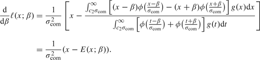
Hence, _MLE that maximizes the conditional likelihood for _com also has conditional expectation equal to _com. Hence, E(β ; _MLE) = _com. Henceforth, we refer to both estimators as _MLE.

The third method proposes an estimator that has the median at the observed _com. This median adjusted estimator is

(3.3)

Intuitively, _Med is the estimate for which the observed _com is the median estimates in the selected SNPs log ORs.

THEOREM 3.2

_Med is median unbiased in sufficiently large samples: (0.5) = β, where (0.5) is the median of _Med.

Proof. Denote _Med = g(_com), therefore, β = g(F⁻¹(0.5)), where F⁻¹(0.5) is the median of the conditional distribution of _com.

THEOREM 3.3

_MLE, _Mean, and _Med are consistent estimators of β (β ≠ 0).

This follows from the fact that the asymptotic distribution of is also an asymptotic approximation to the conditional likelihood of . Therefore, _MLE, _Mean, and _Med are asymptotically equal to the uncorrected , which is a consistent estimator of β.

REMARK 3.1

_MLE, _Mean, and _Med are not regular at β = 0: if β_n = tn_−1/2, then and have distributions dependent on t.

3.2. Weighted average of the corrected estimators and uncorrected estimators

Preliminary simulation studies confirm that uncorrected estimator _com has upward bias but also the corrected estimators, both _MLE and _Med, tend to overcorrect and to underestimate β (as shown in Section 5). Hence, we also considered a linear combination of _com and either of the corrected estimators, denoted by _cor (Chatterjee, written communication). To define weights for this linear combination, we wrote the MSE of _com as the sum of its variance and (β_com − β)², where β_com is the (conditional) mean of _com. The weight for _com is then defined as the ratio of _com², the estimated variance of _com from logistic regression divided by the estimated MSE _com² + (_com − _cor)², whereas the weight for _cor is 1 minus this ratio. This gives an MSE weighted estimator _MSE that is approximately equal to _com, if |_com − _cor| is small and suggestive of little need for correction and is approximately equal to _cor, if |_com − _cor| is large compared to _com²:

(3.4)

where and _cor is either _MLE or _Med. Since both _cor and _com are consistent, _MSE is also consistent.

Each of these estimators is an implicit function of the observed _com. Due to the complexity of the probability density function, there is no closed-form solution for any of them. Rather they can be calculated by a Newton–Raphson root-finding algorithm, and convergence is usually achieved after about 3 iterations starting from _com.

4. SELECTION ADJUSTED CIS

First, a profile CI is developed for the maximum likelihood adjusted estimator _MLE. The log-likelihood is asymptotically χ₁² distributed (assuming underlying β ≠ 0). Thus, the profile confidence limits are the intersection of the log-likelihood curve with a horizontal line χ_1,0.95² / 2 units below its maximum.

Second, similar to the idea of the median adjusted estimator _Med, a quantile-based CI is proposed for _Med as follows. The lower and upper limits for (1 − α)% CI are:

(4.1)

(4.2)

The MSE weighting method can be applied to the confidence limits of the unadjusted CIs and the adjusted CIs to obtain a CI for _MSE. The unadjusted CI is calculated from , where _com is the SE from the logistic regression. The adjusted CI can be either the profile CI or the quantile adjusted CI. Hence,

(4.3)

(4.4)

where and .

5. SIMULATION EVALUATIONS

5.1. Simulation setup

We consider a SNP that is associated with a rare disease. At each simulation, we simulate N case–control pairs. The control group minor allele frequency (p) was set equal to 0.20. Hardy–Weinberg equilibrium was assumed in the control group. Denote by λ the OR corresponding to Z = 1 and θ the OR for Z = 2. Using the rare disease assumption, the case group probabilities for Z = 0, 1, and 2 are then K(1 − p)², 2Kλp(1 − p), and Kθp², where . The multiplicative genetic model (additive on the log scale) was assumed, so that λ = θ^1/2.

For 1-stage designs, all N case–control pairs are used to build the logistic regression of case versus control status on Z. Each SNP was tested at α = 10⁻⁵. For 2-stage designs, a proportion of the case–control pairs are randomly selected for stage 1 and the remaining samples for stage 2. Significance level α₁ = 10⁻² was used for stage 1 selection and _com was tested at α = 10⁻⁵.

For each selected SNP, the uncorrected _com and the corrected estimators _MLE, _Med, and _MSE were estimated according to formulas (3.1), (3.3), and (3.4), respectively. Under a 1-stage design, we also calculated the corrected estimates via the bootstrap method proposed by Sun and Bull (2005) with 1000 bootstrap samples. The unadjusted CI, profile CI, quantile CI, and MSE weighted CI were calculated according to Section 4. At each θ value, 100 significant associations were simulated.

5.2. Simulation results under various β values

Figure 2 shows the bias and the SEs for estimates calculated from SNPs that meet the selection criteria. The results from 1-stage designs are very similar to those from 2-stage designs with equal sample size between the 2 stages. The upward bias is most severe under the null hypothesis. This is because the estimation that is performed conditional on the test statistic exceeds the selection threshold. The absolute value of the naive estimate of the effect size from the same data is at least . Therefore, the uncorrected estimate greatly overestimates the genetic effect for those selected false-positive SNPs. When the true association strength is low, the design has low power and the anticipated upward bias of the uncorrected estimator is evident and most pronounced. For example, when the OR of one copy of risk allele is 1.1, only 1.3% of SNPs were selected, and its bias is 0.215 in a 1-stage design and 0.217 in a 2-stage design. In moderately powered studies, the uncorrected estimate is still clearly biased upward. For example, when OR = 1.3, 66.7% of SNPs were selected. The bias of the uncorrected estimator is 0.040 in a 1-stage design and 0.051 in a 2-stage design. Only in the high-powered study are the estimates centered on the true underlying value. For example, when OR = 1.5, study power is 98%. The bias of the uncorrected estimator is negligible.

Fig. 2.

Simulation results under various heterozygote OR values. Bias and SE of based on 100 significant associations. N = 2000 case–control pairs in 1-stage design, and n = 1000 case–control pairs at each stage in 2-stage design.

In contrast, the average of the corrected estimates is close to the true value, although the estimates are biased slightly downward in small to moderate power situations. Under the null hypothesis, all the proposed corrected estimators have mean values close to zero. The MLE adjusted estimators have smaller bias especially in small OR situation. As noted in Section 3.1, the median adjusted estimators have approximately unbiased medians in all scenarios (not shown in the figure). Its means are very similar to the MLE adjusted estimators, which also have downward bias. The weighted MSE adjusted estimators have the smallest bias among all estimators. Especially, the version that is the weighted average of the uncorrected estimator and the median-corrected estimator is nearly unbiased in all scenarios, except under very small power situation. All the corrected estimates are closer to the uncorrected estimates as study power increases.

We can also observe differences in the variances of the estimates. Figure 2 reveals that the uncorrected estimates for low- and moderately powered studies are tightly clustered around the biased average. The variance of the uncorrected estimates gets larger as OR gets larger. Estimates generated with the corrected method are comparatively more widely dispersed in small and moderately powered situations. The variance of the corrected estimates gets smaller and closer to the variance of the uncorrected estimate at larger ORs. This is expected because the findings from an underpowered study are prone to random errors, and greater uncertainty in point estimation is appropriate, even though not evident with the uncorrected estimator, which tends to take values just above the selection cutpoint. The uncorrected estimators artificially underestimate the variation, while the corrected estimators appropriately recover this uncertainty. The variance of the corrected estimators and the weighted estimators decrease and are closer to that of the uncorrected estimator as study power gets larger.

In general, the corrected estimates are very similar to the uncorrected estimates when the uncorrected estimates are much larger than the selection cutpoint. When a large _com is observed, it very likely comes from a large β value, thus the selection does not have much impact on its distribution. So the uncorrected estimate does not contain much bias, and the corrected estimate therefore is similar to the uncorrected one. However, when the uncorrected estimates are slightly larger than the selection, the selection has a great impact on the distribution of the observed _com. Therefore, the uncorrected _com has a substantial bias (shown in Figure 1). Under this situation, the corrected estimator is much smaller than the uncorrected estimates.

The bootstrap estimate from the approach of Sun and others corrected some bias in the naive estimate but it is still biased upward especially under the null or small power studies. This is consistent with the results shown in Sun and Bull (2006). They explained that when the effect size is small, all sample points of a data set that gives an overall significant result tend to be sampled from the right tail of the true underlying distribution. Thus, the value obtained in the bootstrap sample, which is correlated with the overall sample, overestimates the true effect size (Sun and Bull, 2006).

The coverage rate and CI length are presented in Table 1 in the supplementary material, available at Biostatistics online. The 95% CI coverage rate for the unadjusted estimator ranges from 0% to 98%. Thus, the selection affects the coverage rate, and the amount of reduction in coverage rate is a function of β. The quantile adjusted CIs have coverage rates close to the desired level in all scenarios. The profile CIs are a little conservative in small power studies that the coverage rate is about 98%. But it has similar or shorter length than the quantile adjusted CIs.

Table 2 in the supplementary material, available at Biostatistics online, presents the point estimates performance under various sample size partitioning ratio between the 2 stages while the total sample size is fixed. Varying this ratio between the 2 stages will impact the study power, especially when the underlying OR is small or the first stage sample size is small. A small sample size in the first stage results in a significant loss of power to pick up SNPs for the next stage even when the α level is 0.01. For example, under OR = 1.2 when n₂ / n₁ = 1 / 1, the study power is 12.4%, and the upward bias of _com is 0.110, which is very similar to the power and bias magnitude for a 1-stage design. However, when n₂ / n₁ = 3, the power is about halved, and the upward bias is a slightly larger 0.118. The weighted MSE adjusted estimate _MSE(Med) reduced the bias under all scenarios considered.

5.3. Simulation results on the asymptotic performance under fixed β value

Figure 3 shows additional simulation results with larger sample size to examine the asymptotic performance of the 3 estimators under a fixed heterozygote OR = 1.2. As sample size gets larger, the study power increases, thus the uncorrected estimate has less bias. Again, the MLE-corrected estimates and the median-corrected estimates have smaller bias in small sample size, but overcorrect when sample size is larger. Their downward bias and SE become smaller as sample size increases. Similar to Figure 2, the weighted MSE adjusted estimator using the median adjusted estimate is nearly unbiased except in very small power scenarios. But _MLE and _MSE using the maximum likelihood adjusted estimator have smaller bias when power is extremely low (e.g. N = 1000, study power = 0.78%).

Fig. 3.

Simulation results under various sample size. N is total case–control pairs in 1-stage design and N/2 is case–control pairs at each stage in 2-stage design. Bias and SE of based on 100 significant associations. Heterozygote OR = 1.2.

Table 3 in the supplementary material, available at Biostatistics online, compares the performance of CIs under OR = 1.2 with various sample size. Again, the coverage rates of the unadjusted CIs can be far away from the desired level, while the adjusted CIs have coverage rates close to the nominal level in all scenarios. The adjusted and unadjusted CIs become similar as sample size increases.

6. GENERALIZATION AND DISCUSSION

6.1. The comparison between the _MLE method and the method of Zollner and Pritchard

The method of Zollner and Pritchard (2007) parameterizes the likelihood with 4 parameters: p, minor allele frequency and p₀, p₁, and p₂, the penetrance parameter corresponding to major allele homozygotes, heterozygotes, and minor allele homozygotes. Thus, the parameter that corresponds to β is in their parameterization under the multiplicative OR model assumption and a test for . Because the conditional likelihood function used here is the same concept as that used by Zollner and Pritchard and the maximum likelihood estimate is invariant under 1-1 parameter transformation, from their approach is conceptually very similar to _MLE. However, Zollner and Pritchard use a somewhat different likelihood formulation and seek the MLE via a computational algorithm, while we could use the exact formula provided by the above asymptotic approximations to compute a corrected OR estimator. Another advantage of _MLE is the convenient ability to accommodate additional covariates in the logistic regression.

6.2. Selection bias in

is consistent estimator of σ, even under selection, for any nonzero β. Thus, it has sampling variations that is negligible in large samples. But because is calculated from the inverse of the Fisher information matrix with β replaced by , it has slightly upward bias, under selection, as the selected overestimates β in small samples. We examined this from 1-stage design simulation studies. When OR = 1.1, the selected has mean 0.0556, while the has mean 0.0552 if there were no selection. When OR = 1.2, the selected has mean 0.0549, while the has mean 0.0546 without selection. But for OR greater than 1.3, the upward bias in selected is negligible. Therefore, the bias in the selected is very small compared to that in the selected .

We also implemented an iterative bias-correction algorithm to examine the impact of bias in on . In the algorithm, after is corrected, we plugged in the corrected into the Fisher information matrix to calculate the corrected . We then repeated the above procedure until and both achieved convergence. Simulation results showed that the iterative corrected the slight selection bias in , while the iterated corrected is very similar to the “1-step” corrected previously described, with slightly reduced overcorrection. For example, in the above simulation setup, when OR = 1.1, the 1-step _MLE has bias −0.013, the iterative _MLE has bias −0.006, and the iterative corrected _MLE is 0.0552. When OR = 1.2, the 1-step _MLE has bias −0.041, the iterative _MLE has bias −0.035, and the iterative corrected _MLE is 0.0546. For OR greater than 1.3, there is no detectable difference between 1-step _MLE and the iterative _MLE. Similar pattern is observed for the iterative _Med. Therefore, we concluded that the selection bias in has little impact on the bias-correction procedure for .

6.3. Generalization to multistage designs or other tests

Although the above illustration is based on a 2-stage design, it can be generalized to the designs that have more than 2 stages. At stage i, _i is normally distributed with mean β and independent to all s prior to the stage i. The combined estimator at each stage is defined as , where , with variance . The continuation region at stage i is . At each stage i, if , the SNP can move on to the next stage; otherwise, it stops at stage i. Thus, in a K-stage study, the SNPs that are finally selected are those with . Denote . Its asymptotic approximation can be derived recursively as follows:

Therefore, the probability density function of the combined log OR for the final selected SNPs is

One can further apply the correction method and the adjusted CIs discussed above to this conditional probability density function.

For a biallelic markers, an Armitage trend test (Cochran, 1954; Armitage, 1955) is often used to test for association between the disease probability and the number of minor SNP alleles. The Armitage trend statistic is equivalent to the score statistic for testing H₀: β = 0 in the logistic regression, where Y is the disease status and X is the risk allele count and with no additional covariates (Agresti, 1990). Therefore, the p-values and bias from the Armitage trend statistic can be expected to be very similar to the p-values obtained from the log-additive logistic regression.

6.4. Conclusions

In this paper, we discussed bias-reduction procedure to estimate the SNPs association ORs under GWAS. In GWAS, tens of SNPs may be selected among hundreds of thousands of SNPs tested, and there is not much interest in quantifying associations for unselected SNPs. Rather, conditional inference, including conditional expectation and conditional coverage rate, is pertinent. We demonstrated that the uncorrected estimator _com has very large upward bias in small to moderate power situation. The median corrected estimator _Med and the MLE-corrected estimator _MLE have reduced bias for the selected SNPs when the study power is small. In modest power situations, they tend to overcorrect the bias and have downward bias. The weighted estimator _MSE is nearly unbiased except in very low power scenario. _com severely underestimates the variation of the OR point estimates for the selected SNPs in small power studies, while the corrected estimators recovered the uncertainty in small power studies and have variance that reduces appropriately when study power is large. Selection has very large effects on the coverage rate of the unadjusted CIs regardless the study power. Whereas the profile CIs and the quantile adjusted CIs have coverage rates close to the desired levels under all power scenarios. We conclude that the bias-reduced estimators, especially _MSE and the corresponding selection adjusted CIs, can be recommended for GWAS reporting criteria.

FUNDING

National Institute of Health (CA 53996; CA 106320; CA 86368).

References

- Agresti A. Categorical Data Analysis. New York: Wiley; 1990. [Google Scholar]
- Armitage P. Tests for linear trends in proportions and frequencies. Biometrics. 1955;11:375–386. [Google Scholar]
- Benjamini Y, Hochberg Y. Controlling the false discovery rate: a practical and powerful approach to multiple testing. Journal of the Royal Statistical Society, Series B (Methodological) 1995;57:289–300. [Google Scholar]
- Capen EC, Clapp RV, Campbell WM. Competitive bidding in high-risk situations. Journal of Petroleum Technology. 1971;23:641–653. [Google Scholar]
- Cochran WG. Some methods for strengthening the common chi-square tests. Biometrics. 1954;10:417–451. [Google Scholar]
- Easton DF, Pooley KA, Dunning AM, Pharoah PD, Thompson D, Ballinger DG, Struewing JP, Morrison J, Field H, Luben R. Genome-wide association study identifies novel breast cancer susceptibility loci. Nature. 2007;447:1087–1093. doi: 10.1038/nature05887. [DOI] [PMC free article] [PubMed] [Google Scholar]
- Galton F. Regression towards mediocrity in hereditary stature. Journal of the Anthropological Institute. 1886;15:246–263. [Google Scholar]
- Garner C. Upward bias in odds ratio estimates from genome-wide association studies. Genetic Epidemiology. 2007;31:288–295. doi: 10.1002/gepi.20209. [DOI] [PubMed] [Google Scholar]
- Hunter DJ, Kraft P, Jacobs KB, Cox DG, Yeager M, Hankinson SE, Wacholder S, Wang Z, Welch R, Hutchinson A. A genome-wide association study identifies alleles in FGFR2 associated with risk of sporadic postmenopausal breast cancer. Nature Genetics. 2007;39:870–874. doi: 10.1038/ng2075. [DOI] [PMC free article] [PubMed] [Google Scholar]
- Prentice RL, Qi LH. Aspects of the design and analysis of high-dimensional SNP studies for disease risk estimation. Biostatistics. 2006;7:339–354. doi: 10.1093/biostatistics/kxj020. [DOI] [PubMed] [Google Scholar]
- Risch N, Merikangas K. The future of genetic studies of complex human diseases. Science. 1996;273:1516–1517. doi: 10.1126/science.273.5281.1516. [DOI] [PubMed] [Google Scholar]
- Samani NJ, Erdmann J, Hall AS, Hengstenberg C, Mangino M, Mayer B, Dixon RJ, Meitinger T, Braund P, Wichmann H-E. Genomewide association analysis of coronary artery disease. New England Journal of Medicine. 2007;357:443–453. doi: 10.1056/NEJMoa072366. [DOI] [PMC free article] [PubMed] [Google Scholar]
- Siegmund D. Upward bias in estimation of genetic effect. American Journal of Human Genetics. 2002;71:1184–1188. doi: 10.1086/343819. [DOI] [PMC free article] [PubMed] [Google Scholar]
- Skol AD, Scott LJ, Abecasis GR, Boehnke M. Joint analysis is more efficient than replication-based analysis for two-stage genome-wide association studies. Nature Genetics. 2006;38:209–213. doi: 10.1038/ng1706. [DOI] [PubMed] [Google Scholar]
- Sun L, Bull S. Reduction of selection bias in genomewide studies by resampling. Genetic Epidemiology. 2005;28:352–367. doi: 10.1002/gepi.20068. [DOI] [PubMed] [Google Scholar]
- The Wellcome Trust Case Control Consortium. Genome-wide association study of 14,000 cases of seven common diseases and 3,000 shared controls. Nature. 2007;447:661–678. doi: 10.1038/nature05911. [DOI] [PMC free article] [PubMed] [Google Scholar]
- Whitehead J. On the bias of maximum likelihood estimation following a sequential test. Biometrika. 1986;73:461–471. [Google Scholar]
- Wu LY, Sun L, Bull SB. Locus-specific heritability estimation via the bootstrap in linkage scans for quantitative trait loci. Human Heredity. 2006;62:84–96. doi: 10.1159/000096096. [DOI] [PubMed] [Google Scholar]
- Yu K, Chatterjee N, Wheelerb W, Lia Q, Wang S, Rothman N, Wacholder S. Flexible design for following up positive findings. American Journal of Human Genetics. 2007;81:540–551. doi: 10.1086/520678. [DOI] [PMC free article] [PubMed] [Google Scholar]
- Zollner S, Pritchard J. Overcoming the winners curse: estimating penetrance parameters from case-control data. American Journal of Human Genetics. 2007;80:605–615. doi: 10.1086/512821. [DOI] [PMC free article] [PubMed] [Google Scholar]
Associated Data
This section collects any data citations, data availability statements, or supplementary materials included in this article.