Combinatorial decomposition of an outbreak signature

Abstract

We use mathematically rigorous definitions of epidemiological concepts in order to derive a sequential combinatorial model of disease outbreak decomposition. We define the idea of a population specific ‘disease signature’ and use this in order to decompose and further understand outbreaks as incidents of spatial and temporal spread of disease exposure both in, and across, populations. This allows us to differentiate between different disease spread scenarios with a level of sensitivity that previous models were unable to provide. This perspective leads us to propose a new practical definition for ‘outbreak’. In addition, we are able to use this model to understand, estimate, and, in some cases, correct for, the likely instances of reporting error inherent in disease surveillance.

We demonstrate our model first with a hypothetical outbreak scenario and then in an analysis of suspected outbreaks of waterborne diseases in Massachusetts (MA) in 1995.

1. Introduction

Mathematical models have long been recognized as useful epidemiological tools. They provide a foundation for quantitative predictions, allow for rigorous testing of hypotheses, and necessitate clear definitions of concepts and parameters. The complicated and diverse array of infectious diseases lead to the generation of generalized models that need to be tailored by the use of carefully generated parameters to provide direct insight into the mechanisms of transmission of a particular pathogen, the rate of infection and likelihood of widespread outbreak given certain circumstances, all of which have direct applications for health care management and disease control. Traditionally, these tailored parameters have been mass action transfer terms governing the respective likelihoods of an individual transitioning from susceptible to infected to recovered over time (SIR models, cf. [1]). In cases involving complex circumstances such as multiple distinct populations or repeated, isolated exposures, these models can become complicated, the determination of appropriate mass action terms for each separate population can be difficult [2] and, in some cases, the use of mass action terms themselves can be inappropriate for the focus of the investigation [3]. Additionally, while these mass action transfer terms are mathematically meaningful, they are clinically difficult to measure, creating a disparity between mathematical elegance and usefulness.

By focusing our models on a narrower set of pathogens, those where the link between exposure and infection is clearly defined (as opposed to diseases where there can be multiple and confounding factors), we are able to use the timing of disease incidence and different etiologies specific to the different affected subpopulations to fully understand the dynamics of disease outbreaks. We here propose a method of sequential combinatorial decomposition to accomplish this narrower focus, allowing us to incorporate an understanding of the different temporal distributions governing the transition from susceptible to infected to recovered associated with each population. This method embodies a compromise between the complexity of individual behavior and the broad-brush assumption of mass action, population averages, and is based on a set of clinically measurable parameters. Our system of choice for this study will be waterborne illness due to the clearly defined direct link between exposure and infection. While we have chosen this system for study here, this method may be applied to any system so long as that link is unambiguously understood. All implications of our model are meant to be representative only of this type of system, though the theory may be generalized to others.

Unlike most SIR models that focus solely or primarily on secondary (human-to-human) transmission, we emphasize primary transmission for waterborne illnesses (i.e. an infection from an environmental contaminant/external point source). This is an important aspect because many waterborne diseases have this sort of external transmission that at least sparks an outbreak. We here present a set of rigorous definitions and operational rules that lead to a natural characterization of disease spread. This provides an outbreak signature decomposition model through heterogeneous populations. Additionally, our model will provide a natural, practical, mathematical definition of an ‘outbreak’. We will present our method by analyzing both data from a simulated scenario and actual data from the suspected cryptosporidiosis and giardiasis outbreaks in Massachusetts, USA during 1995 [4].

2. Motivation and rationale

In contrast to other diseases, the waterborne illnesses giardiasis and cryptosporidiosis are prototypical emerging diseases. Both are caused by microscopic parasites in the intestine and are passed in the stool of those infected, contaminating soil, food, or water. Cryptospordiosis has both a small inoculum for humans [5,6] and a large animal reservoir [7]. Both cryptosporidiosis and giardiasis have high rates of exposure once contamination is present in a population, and high rates of infection given exposure. Large proportions of those infected with either disease remain asymptomatic [8]. Those who do exhibit symptoms are likely among specific subpopulations, such as children, elderly, pregnant women, or those who are in some way immunocompromised [9]. However, even in these populations, reporting is often poor. Together, these factors explain relatively few endemic cases detectable by the existing surveillance systems. The need for better surveillance for cryptosporidiosis was made clear during the 1993 outbreak in Milwaukee, which made 403,000 people ill. Only 12 ill people out of a sample of 250,000 people contacted by the CDC were reported to have had cryptosporidiosis via the in-place surveillance system (1 out of ∼20,000 people) [10]. Similar arguments make the same need clear for giardiasis.

Cryptosporidiosis has a low mortality rate and confers only a partial immunity with a 3–6 month turnover [8]. This allows for repeated outbreaks in the same population over a 1 yr cycle, given sufficient time lag between them. (The mortality rate for giardiasis is also low, but nothing is known about its potential to generate partial or long-term immunity.) Outbreaks can be synchronized over time, leading to a seasonal pattern that could be tied to environmental contamination of water supplies, which may be dependent on such factors as rainfall and temperature. These properties make studying ‘endemic levels’ of either giardiasis or cryptosporidiosis in water supplies [4], and therefore in any population served by them, difficult. As a result, many models of waterborne pathogens examine the phenomenon of disease ‘outbreak’, rather than ‘normal endemic levels’ [11]. Since separation between the two is arbitrary and artificial, a model that attempts to describe or predict the manifestation of disease as a natural process must treat exposure and infection in the same way, regardless of whether or not the numbers of infected constitute an ‘outbreak’.

Transmission of either pathogen can occur via two distinct pathways: primary transmission, which involves environmental contamination (such as a contaminated well, recreational water, or drinking water treatment facility), and secondary transmission, which involves direct transfer of the pathogen from host to host [12]. The relative contribution of each method of transmission to the overall levels of exposure can drastically affect the behavior of the pathogen in a population [13].

The distinction between the two processes: endemic and epidemic, presents us with another problem. The CDC sanctioned definition of a waterborne outbreak begins as “an outbreak can generally be defined as a sudden increase in the incidence of disease in a defined area over a specific time” [14]. This is not particularly rigorous, leaving us faced with the problem of how to define an outbreak mathematically. With no recognized standard, the boundary between ‘outbreak’ and ‘non-outbreak’ blurs and an ‘outbreak-specific’ model may, unintentionally, be applied to spikes in endemic fluctuation. Traditionally, SIR models define outbreaks at the point where the reproductive value, R₀, is greater than one. However, while this does provide a theoretical distinction, it may not provide a useful metric. For example, suppose a single person contracts a waterborne illness while traveling, then returns home and successfully transmits the pathogen to the five other people in their immediate family only. Although the pathogen has now infected a total of only six people, the R₀ is such that technically at that point in time, an outbreak has occurred. While the theoretical threshold has been exceeded, the knowledge of that excess does not advance a practical understanding of whether or not a greater population is at risk. This concept can be further refined by broadening the idea of R₀ to apply to ‘major’ (R₀ ≥ 1) and ‘minor’ (R₀ < 1) outbreaks, rather than as a Boolean test of whether or not an outbreak has occurred (cf. [15]). However, again, for each of these definitions relying on R₀ to accurately represent the condition of the spread of disease, they are applied retrospectively, by themselves providing no practical information about the threat of future spread. Instead of a purely theoretical definition, we propose an equally rigorous definition in conjunction with a method for estimating and precisely characterizing disease outbreaks, and the population specific parameters involved. Ultimately, we can then provide the ability to predict both the endemic and epidemic fluctuations of disease incidence.

3. Outbreak signature as a composite of component disease signatures

In the interest of providing a more practical metric, every outbreak can be described as a series of separate events in time and space [4,16]. Each has a set of characteristics that may distinguish it from others, even of the same pathogenic source: duration of the outbreak, magnitude, the overall shape, etc. Together, these traits create an outbreak signature which mathematical models may be used to reproduce or even predict [17,18]. By using the specific properties of the disease (transmission rates, manifestation, etc.) as parameters to generate a ‘disease signature’ comprised of a portfolio of attributes (specific to demographic sub-population), we can think of both endemic levels and, more importantly, outbreaks as a composition of disease signature curves. Similarly, we can construct a model which fits the signature of an outbreak and can yield better understanding of the circumstances which led to it in the first place including how the particular disease signature, host population, and environment affected its spread.

By considering the outbreak signature as a composite of component disease signatures, derived by incorporating spatial and temporal spread into the model itself, we are able to better interpret and trust the parameters that yield the best fit of our model to an outbreak signature curve. Traditional models use average transition probabilities of becoming infected and then recovering, and are not intended to isolate the separate, population-specific distinctions. For example, suppose a traditional Susceptible-Infected-Recovered model [1] of any infectious disease. Suppose the reporting population consists of two etiologically distinct sub-populations, X and Y, exposed to a pathogen at the same time. If the majority sub-population, X, is less susceptible to the disease than the minority sub-population, Y, and they are then arbitrarily aggregated (X + Y), then by treating the outbreak signature as a single curve, then the overall transmission rate may be artificially lowered and the incubation time artificially lengthened. With some prior understanding of the etiology of the disease, we may know how to correct for this in our interpretation of the SIR model, but it does not change the use of averages in the model itself, requiring the definition of an entirely different subpopulation, complete with its own set of mass action transfer values (e.g. [19-22]).

By interpreting the same scenario using the idea of disease signatures, it may quickly become obvious that the outbreak must have acted on two distinct populations. We are then able to use simple combinatorial methods in order to explore which different combinations of sub-curves may have occurred either together, or in sequence, in order to have generated the outbreak signature observed. This allows us a more detailed understanding of both spatial and temporal spread scenarios than is possible by more traditional methods (although it is important to note that spatial complexity can itself be thought of as isolated subpopulations, i.e. if population X is spatially separated from population Y, then the probability of transmission from an infected individual in population X to one in Y is smaller than internal transmission probabilities within each population itself). While each outbreak signature is by no means the result of only one possible combination of component sub-curves, we are able to construct a set of plausible, realistic scenarios from which our signature might have sprung.

4. Modeling strategy

4.1. Basic model formulation

The parameter and variable notation in traditional SIR models lend themselves naturally to mathematical formulation of epidemiological processes, however, these formulations are not always of equal facility in clinical practice or public health surveillance (either for discussion or for practical measurement). Fundamentally, all studies of disease spread rely on composites of underlying etiological and population-specific parameters. In order to foster greater facility in communication among the disciplines, and to make explicit the connections between the standard mathematical formulations and the standard rates measured as part of public health surveillance practice, we formulate our model using the most basic units of etiology and demography. More complex concepts can then be expressed as composites of these units. In fact, many of the familiar parameters from SIR models can be directly computed using these building blocks. We therefore define the following:

• E(X, T) = Probability of being exposed in a given population X at time T.

• I = Probability of becoming infected from exposure.

• S(T) = Probability that, having been infected at time 0, symptoms manifest T days later. (Note: This is a distribution function, which does not need to sum to 1 if not all those infected develop symptoms; this incorporates any latent period and therefore provides a theoretical equivalent to the ‘Exposed’ class in the traditional SEIR models.)

• X_T = The size of the population possibly exposed to infection on day T.

Together, these parameters comprise what we will call the disease signature, N_T, for a particular disease. Assume there is contamination in the population (hence the possibility of exposure) for only one day T₀. Then in a naïve population with an initial population size of X_T0 , the fundamental curve is the number of newly sick on day T defined by N_T = X_T0 (E(X_T0, T₀) * I * S (T − T₀)).

We then consider any outbreak signature as a composite of many disease signature curves. Multiple days of contamination in a population, even from the same source, are considered as different curves, with different T₀ values. We can then iteratively define X_T0+n = X_T0 − X_T0+n−1 (E(x_T0+n−1, T₀ + n− 1) * I). (It is important to note that, if different populations are exposed on ferent days, the disease signature curves will not overlap, due to the definition of X_T0.) Then the composition of those curves yields the following expression, C_T, describing the outbreak signature as:

$$C_T=\underset{n=0}{\overset{T-T_0}{\Sigma }}{X}_{T_0+n}(E(X_{T_0+n},T_0+n)\ast I\ast S(T-T_0+n)).$$

Both I and S(T) can depend on the demographic distribution of the population and will directly affect the shape of the disease signature. If the demography of the population is known, further decomposing N_T into N_T,Y = X_T0,Y (E(X_T0,T₀) * I_Y * S_Y (T − T₀)) for Y = each demographic group (e.g. elderly), provides a more accurate set of curves which, together, make up the disease signature. This yields

$$C_{T,Y}=\underset{\forall Y}{\Sigma }\underset{n=0}{\overset{T-T_0}{\Sigma }}{X}_{T_0+n,Y}(E(X_{T_0+n},T_0+n)\ast I_Y\ast S_Y(T-T_0+n)).$$

Now suppose we want to incorporate re-infection into the fundamental curve, we may either change I on average for each member of the population X_T, or, we may split up X_T into two sub-populations:

Sub-population 1: $X_T^1$ = The size of the population who have either never been infected before day T or have been infected most recently long enough before day T that their possibility of having a decreased susceptibility on day T is near 0.

Sub-population 2: $X_T^2$ = The size of the population who have been infected recently enough before day T to have a decreased probability of infection from current exposure. (Note that this decrease in the probability of infection is assumed to be uniform over the entire population.)

Here, again, this model has been tailored to fit only a very narrow spectrum of waterborne pathogens for which there is the possibility of reinfection, making it distinct from models of diseases generating long term or permanent immunity (e.g., cholera). This type of iterative methodology has been introduced earlier (e.g. [23]); and we have here specifically tailored the formulation of the model to diseases favoring routes of primary transmission. It is also important to note that the traditionally defined standard epidemiological transmission rate can be seen as a combination of these terms we introduced [24].

We also need the additional definition:

• I(T) = Probability of becoming infected from exposure, given previous infection T days ago.

• • T* = Last day of most recent prior infection.

We may then write the more complicated fundamental curve

$$N_T=\left(X_{T_0}^1(E(X_{T_0},T_0)\ast I\ast S(T-T_0))\right)+(X_{T_0}^{2}E(X_{T_0},T_0)\ast I(T-T^{\ast })\ast S(T-T_0)),$$

to incorporate the further complexities of reinfection. Here we adapted the concept suggested in the literature (e.g. [25]), and reformulated it specifically in order to examine primary transmission.

Remark. $X_T^2$ can be broken into as many time segments as needed to maintain the uniformity of the decreased probability of infection, down to daily counts, and would then be written as a set of $X_{(T,T^{\ast })}^2$.

Considering re-infection in the expression of our outbreak signature then yields:

$$\begin{array}{cc}\hfill C_T=& \underset{n=0}{\overset{T-T_0}{\Sigma }}{X}_{T_0+n}^1(E(X_{T_0+n}^1,T_0+n)\ast I\ast S(T-T_0+n))\hfill \\ \hfill & +\underset{m=0}{\overset{T_0}{\Sigma }}\underset{n=0}{\overset{T-T_0}{\Sigma }}{X}_{(T_0+n,m)}^2(E(X_{T_0+n}^2,T_0+n)\ast I(T-m)\ast S(T-T_0+n)).\hfill \end{array}$$

Given this expression, if we define T^Max to be the greatest T for which S(T) ≥ 0 in any subpopulation, and if there is contamination in the population for a finite length of time, then T^Max + 1 days after the last presence of contamination in a population (taken over all demographic subpopulations) there will be no further manifestation of infection. Therefore, maintaining a nonzero endemic level, or any form of sustained outbreak, requires the continued presence of a source of contamination, by either primary or secondary transmission (in the case of secondary transmission, contagious individuals may be themselves be considered the source of contamination). Also, as we have already noted, different subpopulations can lead to different S(T) curves. The different shapes of these curves directly affect the outbreak signature, since it is comprised of their composition.

From an initial set of Q sub-populations (assuming for simplicity that there is no re-infection), the number of possible spread scenarios is Q!. If we wish to incorporate reinfection of sub-populations over i days, the maximum becomes (Qⁱ)!. While this is computationally large, if we are able to make some assumptions about the relative likelihood of certain sub-populations being exposed together (for instance, different demographies being served by the same water supply system), then we are able to reduce the initial estimation of (Qⁱ)!. Additionally, for each day i of the outbreak signature reported, we are able to eliminate all combinations of sub-population curves which significantly over or under estimate the expected number of reported cases, not only for day i, but also for all prior days (subject to the duration of their respective S(T) curves). This implies that the number of possible combinations for consideration is reduced on average by (Q^j) for each day j of reported data. (Note that this reduction will frequently be smaller at the beginning of the data when less is known and larger during the middle and end, when earlier portions of the curve have already been determined, leaving us with only a remaining ((Q – R)^(j–i))! possibilities, where R is the number of sub-populations already contributing to day j.) In this way, we can generate a set of possible spread scenarios over the total population represented in the reported case curve over time.

4.2. A natural definition of an outbreak

Using this idea of an outbreak signature as a composite of component fundamental curves leads us to a natural definition of an outbreak itself, when either of the following is true: (1) The probability of exposure increases by more than one standard deviation from the expected average in at least one population, or (2) when the number of people open to possible exposure to infection at a given time is more than one standard deviation from the expected average. This definition provides a clear point, in advance of the first onset of symptoms, when epidemiologists may agree that a non-endemic progression (or ‘major outbreak’) has begun. While R₀ provides a theoretical threshold, this new definition provides a point of recognition for potential threats earlier in the progress of an outbreak, possibly allowing for earlier intervention.

Suppose that, in a given population, it is highly unlikely for a pathogen to achieve a high rate of secondary transmission. If the probabilities of exposure and infection from a single source of contamination are uniform, and among the population that becomes symptomatic, those symptoms manifest according to a Poisson distribution (in other words, S(T) is Poisson distributed), then if there is a constant level of contamination in a given water supply, we would expect any non-zero endemic level of disease would present newly symptomatic patients according to a periodic Poisson process. It is necessary to assume low rates of secondary transmission in order to eliminate the possibility that spikes in the curve are being produced, not by any Poisson process of becoming infected and symptomatic in the population, but instead are the manifestation of infection having entered a subpopulation with an inherently higher rate of secondary transmission.

It may be possible to distinguish between the two probabilistically by examining the distribution of new cases in close proximity to the local maxima of the peaks. If those local areas themselves show a shape that decomposes into the disease signature curve for subpopulations with high secondary transmission (such as elderly in nursing homes, or children in day-care), then there is reasonable support to believe that a uniform probability has introduced infection into such a population and thereby produced the peak in the endemic fluctuation. However, by our new definition of an outbreak, we notice that, in either of these cases, though there are a greater number of newly symptomatic cases, we have clearly remained in the realm of standard endemic fluctuation.

4.3. Combinatorial decomposition

When using these methods to decompose actual data, it is first necessary to smooth the curve representing the daily number of newly reported cases, especially because weekends can result in artificial zeros. For our smoothing algorithm, if H_i = the actual number of reported cases on a given day i, we chose y_i in order to minimize the following expression: ${\Sigma }_{i=j}^{j+10}(H_i-y_i)2$ over a ten day window. The value was computed using a non-linear gradient search method in MS Excel Solver. The initial j values were chosen at random for each iteration and the computation was allowed to run until the number of i's for which |H_i – y_i| < 100 was greater than 85%.

This method was applied first to a simulated scenario (see Table 1 for all parameter values) and secondly to actual reported case incidence curves from three cities in Massachusetts in 1995 (see Table 2 for parameter values associated with this data). (For a detailed discussion of the suspected outbreak of cryptosporidiosis in Worcester, see [26]).

Table 1.

Hypothetical parameter values for use in simulated decomposition scenario

Parameter	Estimate
Hypothetical scenario
S(T) for adults	Poisson distributed around a mean of 7.5 days
S(T) for children and elderly	Poisson distributed around a mean of 5.5 days
I for adults	0.7
I for children	0.9
I for elderly	0.8
E(Town 1,4)	0.02
E(Town 2,6)	0.01
E(Town 3,8)	0.03
E(X,T) for all other towns and days	0
Town 1 ratio of adults to children to elderly	71:18:11
Town 2 ratio of adults to children to elderly	61:24:15
Town 3 ratio of adults to children to elderly	67:22:11
Total population town 1	560,000.00
Total population town 2	165,000.00
Total population town 3	90,000.00

The values used are assumed for purposes of demonstration and are not related to information about any particular disease.

Table 2.

Actual values estimated for use in decomposition of suspected 1995 MA waterborne disease outbreaks

Massachusetts Cryptosporidiosis and Giardiasis, 1995
Parameter	Estimate	Reference
S(T) for cryptosporidiosis in adults	Poisson distributed around a mean of 7.5 days	Reporteda
S(T) for cryptosporidiosis in children and elderly	Poisson distributed around a mean of 5.5 days	Reporteda,b
S(T) for giardiasis in adults	Poisson distributed around a mean of 10.5 days	Reporteda
S(T) for giardiasis in children and elderly	Poisson distributed around a mean of 8.5 days	Reporteda,b
I for both diseases in adults	0.7	Assumed
I for both diseases in children	0.9	Assumed
I for both diseases in elderly	0.8	Assumed
E(X,T) for all towns and days	1 if contaminant present, 0 otherwise	Assumed for ease of interpretation
Boston ratio of adults to children to elderly	70:20:10	Reportedc
Worcester ratio of adults to children to elderly	62:24:14	Reportedc
Lowell ratio of adults to children to elderly	62:27:11	Reportedc
Total population Boston	589,138.00	Reportedc
Total population Worcester	172,474.00	Reportedc
Total population Lowell	105,167.00	Reportedc

Note that by defining E(X,T) in this way, we incorporate secondary transmission of the disease by considering contamination to be present as a result. These values are taken from empirical studies discussed in the previously published articles cited.

^aRef. [28].

^bRef. [29].

^cRef. [30].

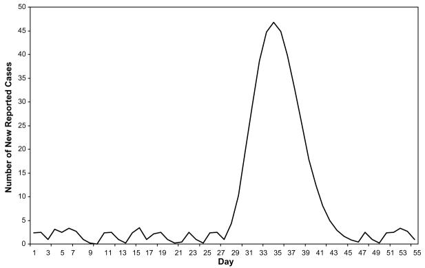
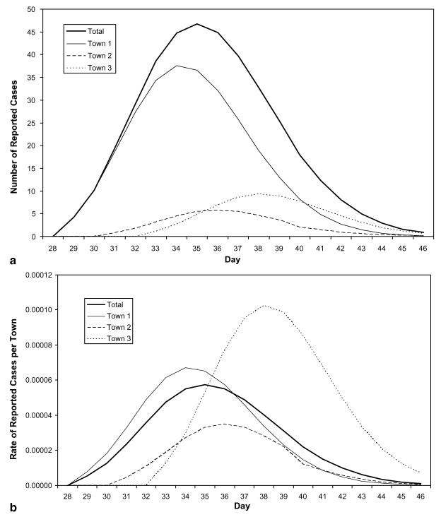
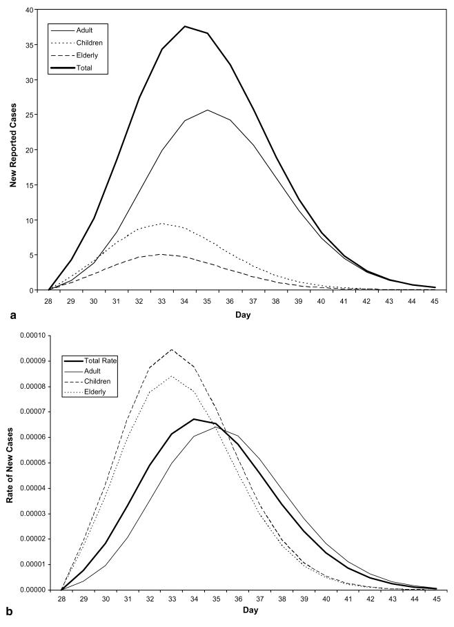
The decomposition of the hypothetical scenario using assumed parameter values from Table 1 yielded the following: A single reporting agency has assembled the daily counts of disease cases from three distinct cities with population sizes of 135 000, 90 000 and 73 000, respectively (see Fig. 1). In this scenario, the geographic decomposition shows that the towns were initially exposed on different days and at varying levels of exposure. By examining both the rates in each city and the counts, we are able to see the relative impact of the disease on each sub-population and the contribution of each sub-population towards the total (see Fig. 2(a) and (b)). Further decomposition of the geographic curves into their demographic component curves again reveals a more exact transmission and temporal spread (see Fig. 3(a) and (b)).

Fig. 1.

Combined reported cases of giardiasis in three hypothetical towns.

Fig. 2.

(a) Number of reported cases – geographic decomposition. The counts are shown here, illustrating each town's contribution to the total reported case count. (b) Rate of reported cases – geographic decomposition. The rates of incidence illustrate the relative prevalence of disease in each town.

Fig. 3.

(a) Demographic decomposition of Town 1. The counts illustrate the contribution of each sub-population to the total reported count for this town. (b) Rate of infection in Town 1 – demographic decomposition. The rates illustrate the difference in prevalence of symptoms in the different sub-populations in the same town, from the same exposure over time.

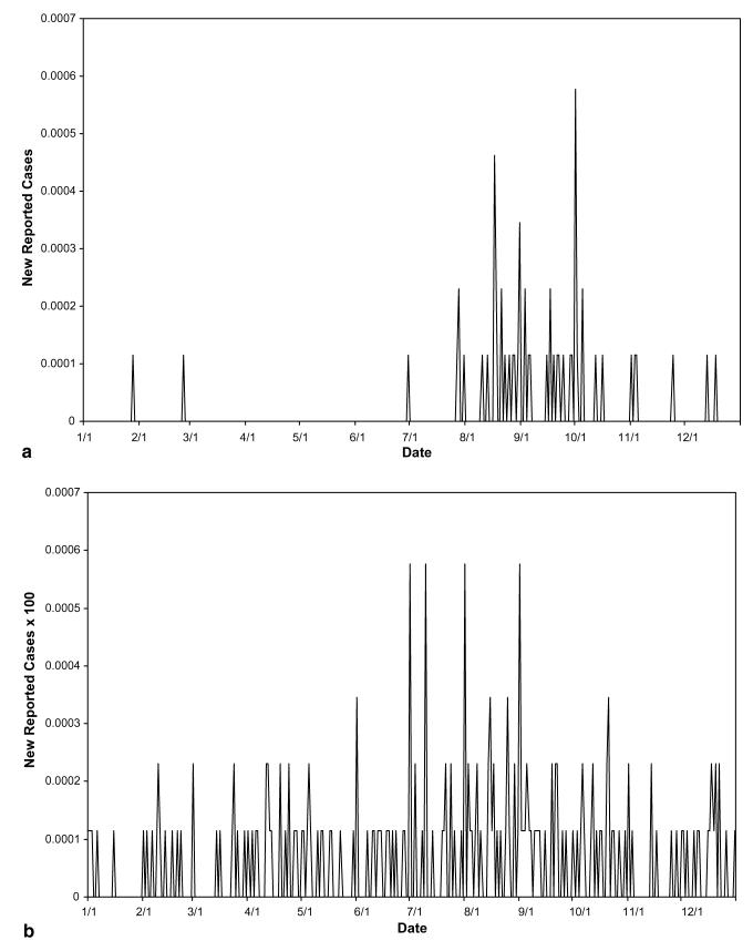
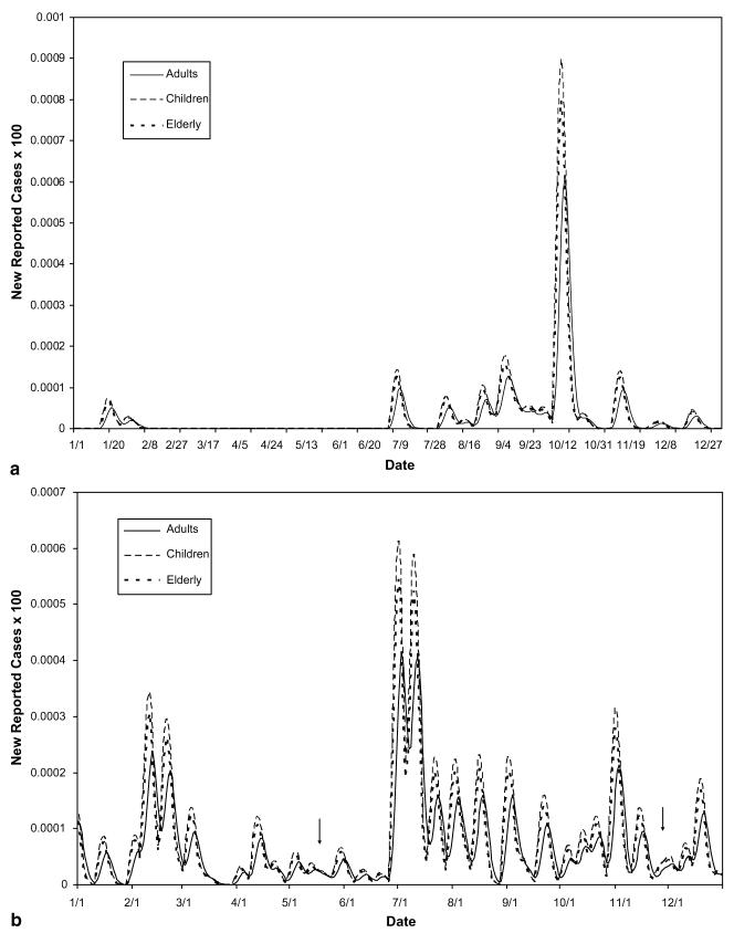
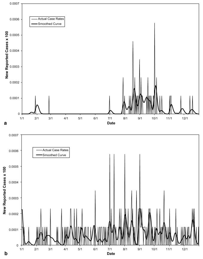
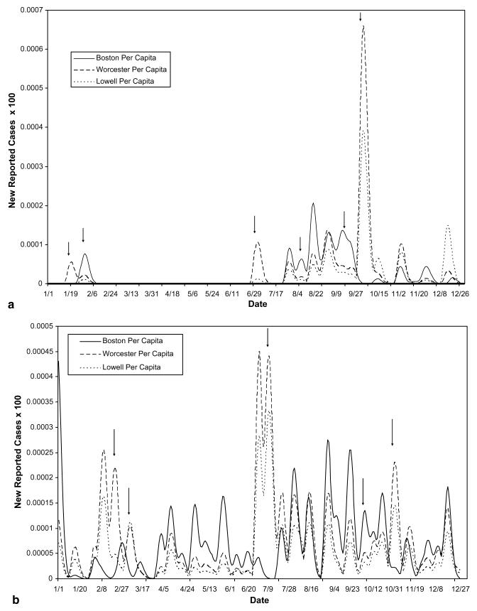
The decomposition of actual reported data from a suspected outbreak of the two waterborne diseases cryptosporidiosis and giardiasis in Boston, Worcester, and Lowell, Massachusetts during 1995, using parameter values listed in Table 2, yielded Figs. 4-8. The original data involved too many zeros to yield a clear decomposition (perhaps in part due to the severe drop in reporting on weekends, causing artificial drops in reported numbers for two out of every five days), it was therefore necessary to smooth the curves for both cryptosporidiosis and giardiasis before decomposition (see Fig. 4(a) and (b), respectively). After smoothing the curves, we obtained the graphs shown in Fig. 5(a) and (b). The geographic decomposition of these data sets show single plausible scenarios of the possible different levels of exposure, over time, in the different cities, to the different diseases, which, given reporting error, could have produced the data (see Fig. 6(a) and (b)).

Fig. 4.

(a) Total reported cryptosporidiosis rate per capita in MA during 1995. (b) Total reported giardiasis rate per capita in MA during 1995.

Fig. 8.

(a) Cryptospordisiosis rates in Worcester, MA, for demographic sub-populations in 1995. Other than the slight delay in development of symptoms for adults, each sub-population in Worcester was found to be equally affected. (b) Giardiasis rates in Worcester, MA, for demographic sub-populations in 1995. Arrows highlight areas suggesting that the effects of the disease on the different sub-populations of the disease were not always in constant proportions. These differences would go unnoticed using average mass action transfer terms.

Fig. 5.

(a) Smoothed reported cryptosporidiosis rate per capita in MA during 1995. (b) Total reported giardiasis rate per capita in MA during 1995.

Fig. 6.

(a) Total rates of cryptosporidiosis in 1995 – geographic decomposition. (b) Total rates of giardiasis in 1995 – geographic decomposition. Arrows highlight areas of the decomposition which indicate that the best fit scenario produced by the combinatorial model suggests a differential impact of disease at different times, in the different cities. These differences would go unnoticed using average mass action transfer terms.

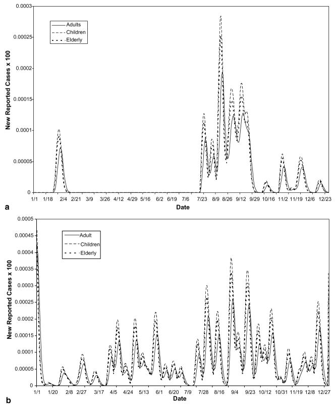
Again, now, we may decompose the case curve for each city by demographic sub-population. Fig. 7(a), (b), 8(a) and (b) demonstrate this for Boston and Worcester, respectively.

Fig. 7.

(a) Cryptosporidiosis rates of reported cases for demographic sub-populations in Boston in 1995. Other than the slight delay in development of symptoms for adults, each sub-population in Boston was found to be equally affected. (b) Giardiasis rates of reported cases for demographic sub-populations in Boston in 1995. Other than the slight delay in development of symptoms for adults, each sub-population in Boston was found to be equally affected.

5. Discussion

This method of combinatorial modeling allows for a careful understanding of the spread of disease through heterogeneous populations, incorporating spatial and temporal complexity. Existing models look at an outbreak as a single curve. In reality, few outbreaks, no matter how they are defined, are isolated enough to be the result of one instance of pathogen contamination into a single, uniform population. This implies that most outbreaks are, in fact, composites of multiple curves, each describing the behavior of one instance of contamination into a single sub-population. We propose that the outbreak signature is therefore comprised of these component curves, overlaid at various times and over various sub-populations. Models that treat the outbreak signature as a single curve, do not ignore this complexity, but incorporate it into the parameters of the model, making it opaque to investigation while ours brings it to the focus of discussion.

For reasons already mentioned in the Introduction, waterborne diseases provide an appropriate system for the demonstration of our approach. However, our modeling methods are in no way specific to any one type of infectious disease. Any disease with a clear and direct link between exposure and infection, leading to reported, symptomatic cases can be decomposed using the same techniques. In fact, some of the most useful applications may well lie in diseases with a more complicated etiology since the differences in their expression in different sub-populations may be more pronounced. This could narrow the number of possible spread scenarios more rapidly than was possible with our waterborne examples.

Another benefit of examining sub-population signature curves, rather than the entire outbreak signature, stems from the high levels of inaccuracy in case reporting for any surveillance based model [27]. If a disease is rare or difficult to diagnose, it can be expected that in the early stages of an outbreak there will be significant under-reporting. Later, after the medical community has been alerted to the possibility of an outbreak, surveillance sensitivity can be expected to increase and may even lead to some false positive reporting. There can also be sub-population specific reporting biases. (It is probably wise for models based solely on reported data to use one well-understood sub-population as a ‘sentinel population’.) Each of these sources of reporting error can lead to inaccurate outbreak estimations and complicate every aspect of outbreak understanding. Studying the effect that these reporting-based corrections have on the observed data can add to our understanding of the actual, rather than the reported, shape of the outbreak curve: the ideal curve. By incorporating estimates of the different potential reporting biases/errors for each different sub-population at a given time into our model, we are able to (at least partially) correct for these sorts of surveillance issues.

With all of the parameters involved in epidemiological modeling, estimations are only as appropriate as reported data and educated intuition together allow. With more and more refined definitions of each sub-population, the likelihood increases that estimations of exposure, susceptibility and symptom manifestation over time, as well as those of reporting bias/error, will closely reflect actual levels. It is also true that, the greater the number of sub-population signature curves possible, the greater the number of possible spatial/temporal scenarios. A trade-off exists between fine tuning the component sub-curves and ‘losing sight of the forest because of the trees’. It is likely that some outbreaks will be most clearly analyzed using sub-populations which are grouped spatially, demographically, or in some other way which lends itself to the mechanism of transmission for the disease in question.

In many cases, estimates of parameters required may have never been studied or reported. In these instances, it may be possible to decompose previously reported outbreak curves using whatever parameters are known in order to educate estimations of those which remain unknown (as was done for a number of our own estimated parameters, see Table 2). It is likely that, here also, there will always be a trade-off between accuracy and efficiency. It may prove an interesting direction for future study to examine the sensitivity of the sequential combinatorial method of modeling disease outbreaks to variation in the rates used to generate the component sub-curve signatures.

Another potential direction for application of this method involves the understanding of the timing of outbreaks in the framework of endemic levels and seasonal patterns of exposure and susceptibility in a population. We hope to explore the possibility of seasonal outbreaks as an artifact of partial immunity, subsequent to a large outbreak, in a given population. By using the disease signatures, we hope to project endemic fluctuations throughout a population as Poisson processes, possibly producing stable cycles of “outbreaks”.

By forming alternative mathematical definitions of epidemiological concepts from a pragmatic perspective and decomposing reported data using these definitions, we are able to understand the progression of an outbreak both through and across populations in a way that other modeling methods do not allow. More comprehensive understanding of the nature of outbreaks can lead to a greater efficacy of surveillance systems that, in turn, can lead to the building of more accurate predictive models. This cycle may eventually lead us to a level of understanding which allows us to propose more effective intervention, or even prevention, systems.

References

- 1.Anderson RM, May RM. Population biology of infectious diseases: Part I. Nature. 1979;280:361. doi: 10.1038/280361a0. [DOI] [PubMed] [Google Scholar]
- 2.Heesterbeek JAP, Roberts MG. Mathematical models for microparasites of wildlife. In: Grenfell BT, Dobson AP, editors. Ecology of Infectious Diseases in Natural Populations. Cambridge University; Cambridge: 1995. [Google Scholar]
- 3.Eubank S, Guclu H, Kumar VSA, Marathe M, Srinivasan A, Toroczkai Z, Wang N. Controlling epidemics in realistic urban social networks. Nature. 2004;429:180. doi: 10.1038/nature02541. [DOI] [PubMed] [Google Scholar]
- 4.Naumova EN, Chen JT, Griffiths JK, Matyas BT, Estes-Smargiassi SA, Morris RD. Use of passive surveillance data to study temporal and spatial variation in the incidence of giardiasis and cryptosporidiosis. Public Health Rep. 2000;115(5):436. doi: 10.1093/phr/115.5.436. [DOI] [PMC free article] [PubMed] [Google Scholar]
- 5.DuPont HL, Chappell CL, Sterling CR, Okhuysen PC, Rose JB, Jakubowski W. The infectivity of Cryptosporidium parvum in healthy volunteers. N. Engl. J. Med. 1995;332(13):855. doi: 10.1056/NEJM199503303321304. [DOI] [PubMed] [Google Scholar]
- 6.Steiner TS, Thielman NM, Guerrant RL. Protozoal agents: what are the dangers for the public water supply? Annu. Rev. Med. 1997;48:329. doi: 10.1146/annurev.med.48.1.329. [DOI] [PubMed] [Google Scholar]
- 7.Tzipori S, Ward H. Cryptosporidiosis: biology, pathogenesis and disease. Microbes Infect. 2002;4(10):1047. doi: 10.1016/s1286-4579(02)01629-5. [DOI] [PubMed] [Google Scholar]
- 8.Griffiths JK. Human cryptosporidiosis: epidemiology, transmission, clinical disease, treatment, and diagnosis. Adv. Parasitol. 1998;40:37. doi: 10.1016/s0065-308x(08)60117-7. [DOI] [PubMed] [Google Scholar]
- 9.Majowicz SE, Michel P, Aramini JJ, McEwen SA, Wilson JB. Descriptive analysis of endemic cryptosporidiosis cases reported in Ontario, 1996–1997. Can. J. Public Health Rev. 2001;92(1):62. doi: 10.1007/BF03404847. [DOI] [PMC free article] [PubMed] [Google Scholar]
- 10.MacKenzie WR, Hoxie NJ, Proctor ME, Gradus MS, Blair KA, Peterson DE, Kazmierczak JJ, Addiss DG, Fox KR, Rose JB, Davis JP. A massive outbreak in Milwaukee of cryptosporidium infection transmitted through the public water supply. N. Engl. J. Med. 1994;331(3):161. doi: 10.1056/NEJM199407213310304. [DOI] [PubMed] [Google Scholar]
- 11.Eisenberg JN, Brookhart MA, Rice G, Brown M, Colford JM., Jr. Disease transmission models for public health decision making: analysis of epidemic and endemic conditions caused by waterborne pathogens. Environ. Health Perspect. 2002;110(8):783. doi: 10.1289/ehp.02110783. [DOI] [PMC free article] [PubMed] [Google Scholar]
- 12.Hunter PR, Colford JM, LeChevallier MW, Binder S, Berger PS. Waterborne diseases. Emerg. Infect. Dis. 2001;7(Suppl 3):544. doi: 10.3201/eid0707.017723. [DOI] [PMC free article] [PubMed] [Google Scholar]
- 13.Koopman JS, Chick SE, Simon CP, Riolo CS, Jacquez G. Stochastic effects on endemic infection levels of disseminating versus local contacts. Math. Biosci. 2002;(180):49. doi: 10.1016/s0025-5564(02)00124-4. [DOI] [PubMed] [Google Scholar]
- 14.Working Group on waterborne cryptosporidiosis, cryptosporidium and water: a public health handbook. Georgia; Atlanta: 1997. [Google Scholar]
- 15.Heres L, Urlings HAP, Wagenaar JA, DeJong MCM. Transmission of Salmonella between broiler chickens fed with fermented liquid feed. Epidemiol. Infect. 2003;132:107. doi: 10.1017/s0950268803001213. [DOI] [PMC free article] [PubMed] [Google Scholar]
- 16.Onstad DW. Temporal and spatial scales in epidemiological concepts. J. Theor. Biol. 1992;158(4):495. doi: 10.1016/s0022-5193(05)80712-x. [DOI] [PubMed] [Google Scholar]
- 17.Naumova EN, MacNeill IB. Signature-forecasting and early outbreak detection system. Environmetrics. 2005;16:749. doi: 10.1002/env.734. [DOI] [PMC free article] [PubMed] [Google Scholar]
- 18.Naumova EN, O'Neil E, MacNeill IB. INFERNO: a system for early outbreak detection and signature forecasting. MMWR. 2005;54(Suppl):77. Available from: < http://www.cdc.gov/mmwr/preview/mmwrhtml/su5401a14.htm>. [PubMed] [Google Scholar]
- 19.Diekmann O, Heesterbeek JAP, Metz JAJ. On the definition and computation of the basic reproduction ratio R0 in models for infectious diseases in heterogeneous populations. J. Math. Biol. 1990;28:365. doi: 10.1007/BF00178324. [DOI] [PubMed] [Google Scholar]
- 20.Roberts MG, Kao RR. The dynamics of an infectious disease in a population with birth pulses. Math. Biosc. 1998;149:23. doi: 10.1016/s0025-5564(97)10016-5. [DOI] [PubMed] [Google Scholar]
- 21.Diekmann O, Heesterbeek JAP. Wiley Series in Mathematical and Computational Biology. John Wiley & Sons; Chichester, UK: 2000. Mathematical epidemiology of infectious diseases: model building, analysis and interpretation. [Google Scholar]
- 22.Fulford GR, Roberts MG, Heesterbeek JAP. The metapopulation dynamics of an infectious disease: tuberculosis in possums. Theor. Pop. Biol. 2002;61:15. doi: 10.1006/tpbi.2001.1553. [DOI] [PubMed] [Google Scholar]
- 23.Finkenstädt BF, Grenfell BT. Time series modelling of childhood diseases: a dynamical systems approach. J.R. Stat. Soc. Ser. C Appl. Stat. 2000;49(1):187. [Google Scholar]
- 24.Roberts M, Heesterbeek H. Bluff your way in epidemic models. Trends Microbiol. 1993;1:343. doi: 10.1016/0966-842x(93)90075-3. [DOI] [PubMed] [Google Scholar]
- 25.Cooke KL, Calef DF, Level EV. Non-linear Systems and its Application. Academic; New York: 1977. [Google Scholar]
- 26.Elam-Evans LD, Kaufmann RB, Schantz PM. Epi-Aid 95-86. CDC; 1996. Investigation of cryptosporidiosis Worcester and surrounding areas. [Google Scholar]
- 27.Proctor ME, Blair KA, Davis JP. Surveillance data for waterborne illness detection: an assessment following a massive waterborne outbreak of Cryptosporidium infection. Epidemiol. Infect. 1998;120:43. doi: 10.1017/s0950268897008327. [DOI] [PMC free article] [PubMed] [Google Scholar]
- 28.Hunter PR. Waterborne Disease: Epidemiology and Ecology. John Wiley & Sons, Public Health Laboratory Service; Chester, UK: 1997. [Google Scholar]
- 29.Naumova EN, Egorov AI, Morris RD, Griffiths JK. The elderly and waterborne Cryptosporidium infection: Gastroenteritis hospitalizations before and during the 1993 Milwaukee outbreak. Emerg. Infect. Dis. 2003;9(4):418. doi: 10.3201/eid0904.020260. [DOI] [PMC free article] [PubMed] [Google Scholar]
- 30.MassCHIP . Massachusetts Department of Public Health; 2003. Available from:< http://www.state.ma.us/dph/>. [Google Scholar]