Spectroscopic and Quantum Chemical Studies on low-spin Fe^IV=O complexes: Fe-O bonding and its contributions to reactivity

Abstract

High valent Fe^IV=O species are key intermediates in the catalytic cycles of many mononuclear non-heme iron enzymes and have been structurally defined in model systems. Variable temperature magnetic circular dichroism (VT-MCD) spectroscopy has been used to evaluate the electronic structures and in particular the Fe-O bonds of three Fe^IV=O (S=1) model complexes, [Fe^IV(O)(TMC)(NCMe)]²⁺, [Fe^IV(O)(TMC)(OC(O)CF₃)]⁺, and [Fe^IV(O)(N4Py)]²⁺. These complexes are characterized by their strong and covalent Fe-O π-bonds. The MCD spectra show a vibronic progression in the non-bonding → π* excited state, providing the Fe-O stretching frequency and the Fe-O bond length in this excited state and quantifying the π-contribution to the total Fe-O bond. Correlation of these experimental data to reactivity shows that the [Fe^IV(O)(N4Py)]²⁺ complex, with the highest reactivity towards hydrogen-atom abstraction among the three, has the strongest Fe-O π-bond.

Density Functional calculations were correlated to the data and support the experimental analysis. The strength and covalency of the Fe-O π-bond result in high oxygen character in the important frontier molecular orbitals (FMOs) for this reaction, the unoccupied β-spin d(xz/yz) orbitals, and activates these for electrophilic attack. An extension to biologically relevant Fe^IV=O (S=2) enzyme intermediates shows that these can perform electrophilic attack reactions along the same mechanistic pathway (π-FMO pathway) with similar reactivity, but also have an additional reaction channel involving the unoccupied α-spin d(z²) orbital (σ-FMO pathway).

These studies experimentally probe the FMOs involved in the reactivity of Fe^IV=O (S=1) model complexes resulting in a detailed understanding of the Fe-O bond and its contributions to reactivity.

1 Introduction

The catalytic pathways of many mononuclear non-heme iron enzymes are proposed to involve a high-valent iron-oxo intermediate as the active oxidizing species.^1,2 Such an intermediate also plays an integral role in many heme enzymatic cycles.^3,4 In non-heme iron enzymes, mononuclear Fe^IV-oxo intermediates have been trapped and characterized for several α-ketoglutarate dependent enzymes: taurine:α-KG dioxygenase (TauD),^5–8 prolyl-4-hydroxylase (P4H),⁹ and most recently for the halogenase CytC3.¹⁰ However, due to their relative instability, their structural characterization has proven challenging.¹¹

Many biomimetic Fe^IV=O model complexes with non-heme ligand sets, all with a six-coordinate axially distorted center and an S = 1 ground state, have now been synthesized and several structurally and spectroscopically studied.^12–25 In addition, an S=2 [Fe^IV(O)(H₂O)₅]²⁺ species has been generated and characterized.^26,27

Computational studies on the qualitative bonding in these mononuclear non-heme Fe^IV S=1 species all result in a very similar electronic structure description (Figure 1) with a (xy)²(xz/yz)² ground configuration.^28–31 The Fe-O bond is formed by interaction between the O-p(z) and the unoccupied iron d(z²) orbitals, resulting in a σ-bond and interactions of the O-p(x/y) orbitals and the ½ occupied iron d(xz/yz) orbitals generating 2×1/2 Fe-O π-bonds. The d(x²-y²) orbital is σ* with respect to the equatorial ligands. The equatorial ligand field strength determines the destabilization and relative energy of the d(x²-y²) orbital and thus the spin of the ground state.

Figure 1.

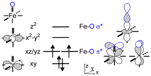
Iron d-based frontier molecular orbitals and Fe-O bonding in non-heme Fe^IV=O (S=1) systems.

However, to validate the computational descriptions, we need to experimentally understand the electronic structure of these Fe=O complexes and in particular the Fe-O bonding. A breakthrough in this direction was achieved with variable-temperature magnetic-circular-dichroism (VT-MCD) spectroscopy,²⁹ which allows polarized spectroscopy on a randomly-oriented frozen powder sample. In addition, vibronic fine-structure was observed for the first time in an iron-oxo species. Through these studies an experimental description of the electronic structure was obtained, defined by a very strong and covalent Fe=O π-bond.

We now extend these experimental studies and, in combination with density functional calculations, use these to:

1. Develop an analysis of the vibronic fine-structure of the [Fe^IV(O)(TMC)(NCMe)]²⁺ complex (1) (Figure 2 left),^13,32 which qualitatively and quantitatively describes the nature of the Fe-O π-bond;

2. Define the effect of variations of the axial and equatorial coordination of the iron. Replacing the axial acetonitrile of complex 1 with an anionic carboxylate ligand forms the [Fe^IV(O)(TMC)(OC(O)CF₃)]⁺ species (2) (Figure 2 center).22 The [Fe^IV(O)(N4Py)]²⁺ complex (3) (Figure 2 right)^16,19,33 has different equatorial ligands with pyridines instead of amines. Interestingly, these three complexes show very different reactivity towards hydrogen-atom abstraction. While 1 and 2 are rather unreactive and only able to break relatively weak C-H bonds (for example in dihydroanthracene),²² 3 is much more reactive and can hydroxylate cyclohexane.¹⁶ The electronic structures of these three complexes are determined in this study and used to understand electronic structure contributions to the differences in their reactivities.

3. Extend these studies to S=2 Fe^IV=O enzyme intermediates to evaluate the variations in reactivity with spin state.

Figure 2.

Structures of the three complexes in this study: 1 [Fe^IV(O)(TMC)(NCMe)]²⁺, 2 [Fe^IV(O)(TMC)(OC(O)CF₃)]⁺, and 3 [Fe^IV(O)(N4Py)]²⁺.

2 Methods

2.1 Sample Preparation

Sample preparation of solid [Fe(O)(TMC)(NCCH₃)](OTf)₂ (1)

Acetonitrile and methanol were dried according to published procedures and distilled under Ar prior to use.³⁴ [Fe(O)(TMC)(NCCH₃)](OTf)₂ was generated as previously described:¹³ A solution of [Fe(TMC)(OTf)]OTf (25.6 mg, 0.042 mmol) in 7 mL acetonitrile was pre-cooled to −40 °C. Addition of a solution of PhIO (9.3 mg, 0.042 mmol) in 350 μL methanol yielded the Fe^IV complex. After 5 min, the product was precipitated by addition of 20 mL pre-cooled diethyl ether. This mixture was allowed to stand for 10 min at −40 °C and centrifuged for 2 min at 0 °C, before the solvents were decanted. The green solid was washed with 5 mL cold diethyl ether and dried in vacuo. The samples were stored in liquid nitrogen.

Sample preparation of [Fe(O)(TMC)(OC(O)CF₃)]OTf (2)

The sample of 2 was generated by oxidation of the corresponding Fe^II precursor, [Fe(TMC)(OC(O)CF₃)]OTf. A solution of [Fe(TMC)(OTf)]OTf (0.018 mmol) and NEt₄CF₃CO₂ (0.018 mmol) in 3.05 mL butyronitrile was prepared in a UV-visible cuvette and pre-cooled to −20 °C. 1.2 equiv of PhIO (0.0216 mmol) in 0.1 mL MeOH were added to this solution. The formation of 2 was shown to be complete within 1 h by monitoring the absorption band at λ_max = 836 nm (ε = 250 M⁻¹cm⁻¹). The samples were stored in liquid nitrogen

Sample preparation of [Fe(O)(N4Py)](ClO₄)₂ (3)

Butyronitrile was purchased from Aldrich and used without further purification. [Fe(N4Py)(NCCH₃)](ClO₄)₂ was prepared according to published methods.³⁵ A 4.0 mM solution of [Fe(N4Py)(NCCH₃)](ClO₄)₂ (13.27 mg, 0.020 mmol) in 5 mL butyronitrile was prepared at room temperature. Excess solid PhIO (15 mg, 0.068 mmol) was added to the solution and the reaction was stirred vigorously for 20 minutes. The reaction mixture was passed through a syringe filter of pore size 0.2 μm to give 3 as a transparent, blue-green solution. A yield of 85(5)% was determined by UV-Vis from the absorption band at 695 nm (ε = 400 M⁻¹ cm⁻¹). The samples were stored in liquid nitrogren.

2.2 Absorption Spectroscopy

UV/Vis spectra were recorded on an HP 8453A diode array spectrometer. Low-temperature visible spectra were obtained using a cryostat from UNISOKU Scientific Instruments, Japan.

2.3 MCD Spectroscopy

The solid samples of complex 1 were prepared by dispersing the solid into an optically transparent mulling agent (fluorolube) which was then sandwiched between two quartz disks and placed in a copper MCD sample cell. The butyronitile solutions of complexes 2 and 3 were injected between two Infrasil quartz disks separated by a 3 mm thick rubber O-ring spacer, held inside the copper MCD sample cell. Typical sample concentrations were in the range of 4–8 mM. The samples were frozen in liquid N₂ immediately after preparation.

The MCD data were collected on CD spectropolarimeters with modified sample compartments to accommodate magnetocryostats. The near-IR spectra were obtained using a Jasco J200-D spectropolarimeter with a liquid N₂-cooled InSb detector equipped with an Oxford Instruments SM4000-7T superconducting magnetocryostat. The UV/visible data were collected on a Jasco 810 spectropolarimeter with S1 and S20 photomultiplier tubes (Hamamatsu) as detectors and equipped with an Oxford Instruments SM4-8T superconducting magnetocryostat. MCD spectra were collected at various fields (7T, 4T, 1T) and several temperatures between 2K and 80K. They are corrected for zero-field baseline effects by subtracting the corresponding 0T scans at each temperature. The Absorption and VT-MCD spectra were simultaneously fit to Gaussian band shapes to determine the transition energies.

2.4 Electronic Structure Calculations

Spin unrestricted DFT calculations were performed with the Gaussian 03³⁶ and Amsterdam Density Functional (ADF 2003.01)^37–39 program packages. The geometries of all three Fe^IV=O complexes (1, 2 and 3) were fully optimized for the S=1 and S=2 states starting from the X-ray geometries of 1¹³ and 3.¹⁹

In ADF the local density approximation (LDA) of Vosko, Wilk and Nussair (VWN)⁴⁰ was used together with gradient corrections for exchange (Becke88)⁴¹ and correlation (Perdew86).⁴² An uncontracted, all electron triple-ζ basis set with a single polarization function (TZP) was employed. Convergence was reached when the maximum element in the error matrix was less than 10⁻⁵. The energies of the electronic transitions were calculated using the ΔSCF method, i.e. each excited state was converged fixed in the ground state geometry, and the energy difference between this electronic excited state and the ground state was calculated, ΔE = E(es) –E(gs). In addition, the geometry of the excited state with the electronic configuration d(xy)¹d(xz/yz)³ was optimized, the wave function converged, but fixed in this electronic excited state. Thus, the structure of the geometrically relaxed excited state was obtained.

The Gaussian calculations were performed with two often used functionals: the BP86 functional using Becke’s 1988 exchange functional⁴³ with the correlation function of Perdew^42,44 and the hybrid B3LYP functional using Becke’s three-parameter hybrid functional with the correlation functional of Lee, Yang, and Parr.^41,45 The LanL2DZ basis set, which applies Dunning/Huzinaga full double-ζ (D95) basis functions on first-row elements⁴⁶ and Los Alamos effective core potentials plus DZ functions on all other atoms,^47–49 were used in all geometry optimizations. Convergence was defined to occur when the relative change in the density matrix between subsequent iterations was less than 1×10⁻⁸. Spin-contaminations were negligible in all cases. Single point calculations were carried out on the optimized geometries using a larger all-electron, triple-ζ basis set with one set of polarization functions on the heavy atoms (6-311G*). All energy values reported result from these triple-ζ basis set calculations. TD-DFT calculations were carried out with the BP86 functional, the same triple-ζ, all electron basis set, 6-311G*, and the direct inclusion of solvation effects using the Polarized Continuum Model (PCM)^50–52 with acetonitrile as the solvent.

Molecular orbital compositions and Mayer Bond Orders were calculated using the PyMOlyze program.⁵³ Orbitals from the Gaussian calculations were plotted using Molden,⁵⁴ from the ADF calculations with gOpenMol. ⁵⁵ The electronic structures and bonding interactions were analyzed by means of the unoccupied antibonding molecular orbitals, which reflect the uncompensated electron density involved in bonding interactions.

The thermodynamics of the H-atom abstraction reaction (with 2,3-dimethylbutane as the H-atom donor) were calculated using the B3LYP functional. The geometries of all reactant and product species have been fully optimized without constraints, and the frequencies were found to be real in all cases. All energies were obtained from single-point calculations on the LanL2DZ-optimized structures using the 6-311G* basis set. The energies given include zero-point and thermal corrections. Solvation effects were included using the Polarized Continuum Model (PCM) with acetonitrile as solvent.

3 Results and Analysis

In this section we present absorption and variable-temperature MCD spectra on the three Fe^IV=O complexes with variations in the axial and equatorial ligation and then compare the experimental trends among the three complexes. Results from density functional calculations will be correlated to the experimental results and the additional insight gained are presented in section 3.5.

3.1 Absorption and MCD spectroscopy

The UV/Vis absorption and MCD spectra (7T, 2K and 7T, 20K) of the three compounds, [Fe^IV(O)(TMC)(NCMe)]²⁺ 1, [Fe^IV(O)(TMC)(OC(O)CF₃)]⁺ 2, and [FeIV(O)(N4Py)]²⁺ 3, in the energy region from 5,000 to 28,000 cm⁻¹ are shown in Figure 3.

Figure 3.

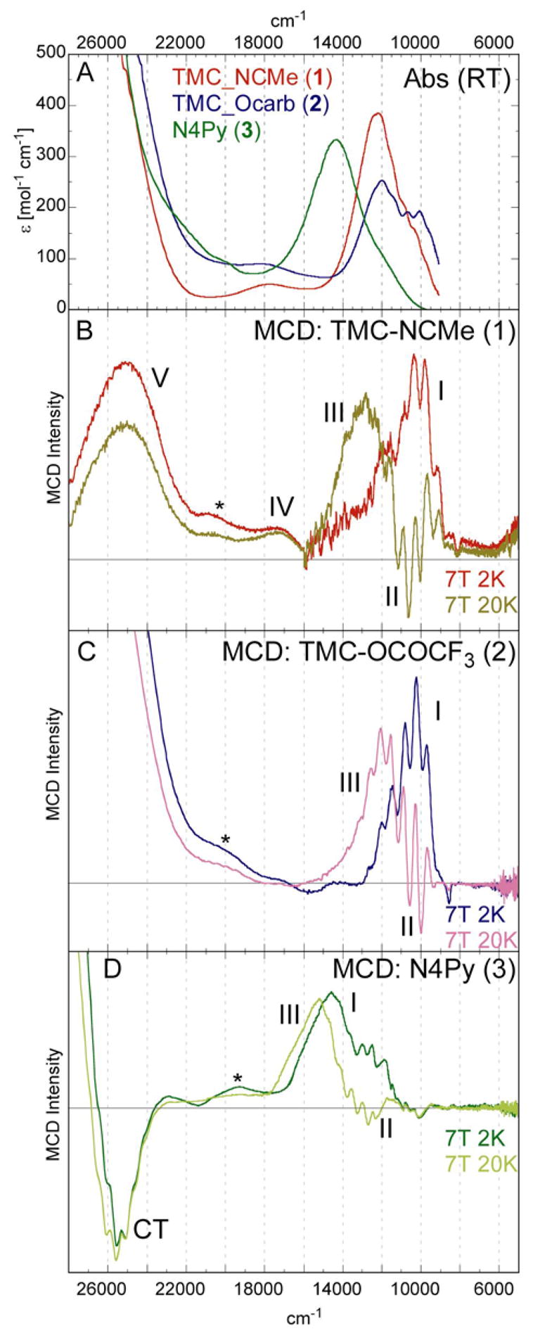
UV/Vis absorption (A) and VT-MCD spectra (overlay of 7T, 2K and 7T, 20K) of [Fe^IV(O)(TMC)(NCMe)]²⁺ (B), [Fe^IV(O)(TMC)(OC(O)CF₃)]⁺ (C), and [Fe^IV(O)(N4Py)]²⁺ (D).

All three absorption spectra (Figure 3 A) show one broad band in the near-IR region, between 11,000 and 15,000 cm⁻¹, then no discernable feature until the absorption intensity increases sharply above 24,000 cm⁻¹, i.e. in the charge transfer region. The near-IR bands of complexes 1 and 2 have very similar energies, ~12,000 cm⁻¹, (Table 1) while the absorption band of 3 is blue-shifted to ~14,400 cm⁻¹. The absorption band of complex 2 has a lower extinction coefficient (ε ~ 250 mol⁻¹cm⁻¹ vs. ε ~ 400 mol⁻¹cm⁻¹ for 3 and 1), and shows a low-energy shoulder, at ~11,000 cm⁻¹, with some fine structure.

Table 1.

Experimental transition energies (in cm⁻¹) according to the UV/Vis absorption and variable-temperature MCD spectra of [Fe^IV(O)(TMC)(NCMe)]²⁺ 1, [Fe^IV(O)(TMC)(OC(O)CF₃)]⁺ 2, and [Fe^IV(O)(N4Py)]²⁺ 3.

		1	2	3
UV/Vis Abs.		~12,100	~12,000 (shoulder ~ 11,000)	~14,400
MCD	I	~10,400	~10,300	~14,000
	II	~10,600	~11,100	~12,600
	III	~12,900	~12,000	~15,100
	IV	~17,600	--	--
	V	~24,900	--	--
	CT	--	--	~25,600

all energies in cm ⁻¹

In the MCD spectra (Figure 3 B,C,D, which overlay the 2K and 20K spectra as there is a large temperature dependence of the MCD signal (see section 3.2)), all three complexes qualitatively show three bands in the lower energy region (5,000 – 18,000 cm⁻¹). Only one band has intensity at low temperatures (2K, band I), and two bands have intensity only at intermediate temperatures (20K, bands II and III). Bands I and III are positive, while band II is negative and shows fine structure. The transition energies are very similar for complexes 1 and 2 (Table 1); bands II and III are shifted only slightly in complex 2 by 500 and 900 cm⁻¹ respectively. Complex 3 shows large differences, with all three bands in the low energy region blue-shifted by at least 2,000 cm⁻¹ compared to complex 1. The largest difference is in band I which is ~3,600 cm⁻¹ higher in energy in complex 3. These shifts in relative energies result in the different shapes of the overall spectra seen in Figure 3.

Correlating the near-IR absorption with the MCD spectra shows that band III is the most intense transition under the broad envelope of the absorption spectra, band II has some absorption intensity, and band I has very little or no absorption intensity. In complex 2 relative to 1 the absorption intensity is redistributed, band III has a lower extinction coefficient, while band II is more intense, resulting in the more pronounced fine structure (vibronic progression, vide infra) in the absorption spectrum.

Above 18,000 cm⁻¹, one low intensity band was identified for complex 1 (IV in Figure 3B). The corresponding band cannot be clearly identified for complexes 2 or 3, as impurities⁵⁶ have transitions in this energy region (* in Figure 3).

At energies above 22,000 cm⁻¹, the MCD spectra of these three complexes are very different. Complex 1 shows a distinct positive band at ~24,900 cm⁻¹ (band V in Figure 3B). In this energy region the MCD intensity of complex 2 increases sharply, so no distinct band can be identified. Complex 3 shows a negative band with fine structure at ~25,600 cm⁻¹ (labeled CT in Figure 3D, vide infra); to higher energies the MCD becomes positive and rises sharply into the UV region.

3.2 Variable-temperature MCD spectra

The details of the temperature dependent behavior of the MCD spectra of bands I, II, and III in the 5,000 – 19,000 cm⁻¹ energy region are shown in Figure 4. For all three complexes, the MCD intensity of band I decreases with increasing temperature, while band II, which is negative in sign and exhibits a vibronic progression (vide infra), and band III have a different temperature behavior. Their intensities first increase in magnitude with increasing temperature, up to a maximum at ~20K, after which the MCD intensities decrease with further increase in temperature. All MCD features show a linear dependence with magnetic field strength.

Figure 4.

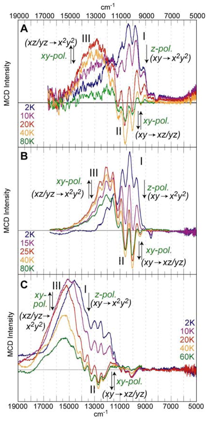
Variable-temperature MCD spectra of complexes 1 (A), 2 (B), and 3 (C) in the energy region from 5,000–19,000 cm⁻¹.

As we have analyzed earlier,²⁹ these different temperature-dependent behaviors in the MCD spectra reflect the different polarizations of the electronic transitions. MCD intensity is proportional to g_iM_jM_k, where g_i is the Zeeman effect in i direction, M_j, M_k are electric dipole transition moments in j, k directions, and i, j, k are cyclic permutations of x, y, z. These complexes were defined by Mössbauer studies^13,16,57 as axially distorted with S = 1 ground states and positive zero-field splittings, D > 0, between the non-degenerate M_S = 0 and the doubly degenerate M_S = ±1 sublevels (Figure 5). For xy-polarized transitions, MCD intensity is present only with the magnetic field H in the molecular z-direction (Figure 5, left). In this field orientation, the M_S = 0 level does not mix with other M_S sublevels, and thus there is no MCD signal at low temperatures. Increasing temperature populates the M_S = ±1 levels, which are MCD active, and xy-polarized transitions gain MCD intensity. At still higher temperatures the MCD intensity decreases with I ~ 1/T according to the Curie behavior. For z-polarized transitions, the magnetic field must be in the molecular xy-plane for MCD intensity (Figure 5, right). In this orientation, the M_S = 0 level mixes with one component of M_S = ±1 and induces M_S = −1 character into the lowest level and hence MCD intensity at low temperatures. Increasing temperature decreases the population of this level and increases the population of the M_S = 0 and M_S = +1 sublevels. Since the MCD signals of the M_S = +1 and M_S = −1 sublevels are of opposite sign, the MCD intensity decreases with increasing temperatures. Thus, starting at low temperatures, xy-polarized transition intensity increases with temperature, while z-polarized transition intensity decreases.²⁹

Figure 5.

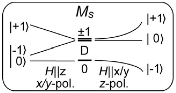
M_s sublevels and MCD selection rules determine temperature-dependent behavior

The temperature behavior of the MCD features allows us to assign polarizations to bands in these randomly oriented samples. In all three complexes, band I corresponds to a z-polarized transition, while bands II and III are xy-polarized transitions. Since band IV (in complex 1) overlaps with band III, its temperature behavior and thus polarization are difficult to distinguish. In the higher energy region (see SI for detailed temperature-dependent spectra) band V of complex 1 and the CT-band of complex 3 are z-polarized.

Thus all three complexes show the same fingerprint in this lower energy region, three bands with the same temperature behavior and signs. We can then apply the assignments of bands I, II and III for complex 1²⁹ to complexes 2 and 3.

According to group theory, a d⁴ S = 1 system with C_4v symmetry has a ³A₂ ground state with five spin allowed, electric dipole allowed d-d ligand field transitions (Figure 6). Specific assignments were made based on the polarizations of the bands deduced from their MCD temperature behavior, the vibronic structure, and their relative intensities in the electronic absorption spectrum (see section 3.1).

Figure 6.

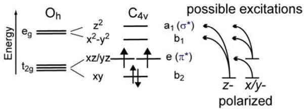
Ligand field splitting diagram and spin- and electric-dipole allowed d-d transitions.

Band I is assigned to the z-polarized d(xy) → d(x²-y²) transition, reflecting the strength of the equatorial ligand field. (Figure 1). The negative band II is xy-polarized and is assigned as the excitation of an electron from the non-bonding (nb) d(xy) to the Fe-O π* d(xz/yz) orbitals. Thus, the energy of this transition is a measure of the covalency and strength of the Fe-O π-bond. The fine structure is associated with this transition and represents the change in this bond in the excited state (see section 3.3). Band III is also xy-polarized and assigned to the d(xz/yz) → d(x²-y²) transition. Its absorption intensity (Figure 3A) results from mixing with a low-lying, intense ligand-to-metal charge-transfer (LMCT) excited state from the equatorial nitrogens to the d(x²-y²) orbital. Band IV is assigned to the d(xz/yz) → d(z²) transition in complex 1. This band cannot be identified in 2 or 3 because of contributions from small impurities in this energy region (Figure 3). Band V which also can only be cleanly observed in complex 1, is z-polarized and assigned to the highest-energy ligand field transition, from the nb d(xy) to the σ* d(z²) orbitals, its energy reflecting the covalency and strength of the Fe-O σ-bond.

This region (~ 24,900 cm⁻¹) is obscured in complex 2 by low energy, very intense transitions in both the absorption and MCD spectra. DFT calculations (see section 3.5) indicate that these transitions in complex 2 are LMCT transitions from the axial carboxylate lone-pair into the iron d(xz/yz) orbitals. In contrast to both 1 and 2, complex 3 shows a very intense, z-polarized, but negative MCD band at ~25,000 cm⁻¹ which has fine structure identical to band II (Figure 3). The assignment of this band is presented in section 3.4.

In the next section we analyze the fine structure of band II, and in section 3.4 compare the experimental trends of the three complexes and interpret these in terms of ligand field effects.

3.3 Analysis of the vibronic progression

As presented above, the negative band II, which has been assigned as the ligand field transition d(xy) → d(xz/yz), shows fine structure in all three complexes, which is a vibronic Franck-Condon progression in the Fe-O stretching mode. The transition involves excitation of an electron from the non-bonding d(xy) orbital into the strongly Fe-O π antibonding d(xz/yz) orbitals eliminating one of the 2×½ Fe-O π-bonds. This weakening of the Fe-O π-bond by this additional electron leads to a distortion (i.e. elongation) of the Fe-O bond length in the excited state, Δr(Fe-O) = r_es(Fe-O) – r_gs(Fe-O), as well as to a reduction in the Fe-O force constant (k) in the excited state, reflected in ν_es(Fe-O), compared to that of the ground state, ν_gs(Fe-O)(Figure 7). The distortion of the excited state geometry relative to that of the ground state, Δr, lowers the energy of Ψ_es by E_Fe-O = ½ k Δr² relative to its value at the Ψ_gs equilibrium geometry.

Figure 7.

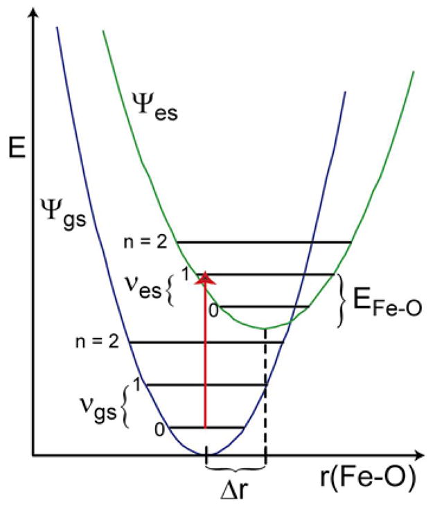
Electronic transition from the electronic and vibrational ground state (Ψ_gs, n = 0) into vibrational levels (n ≥ 0) of the electronic excited state (Ψ_es). The Ψ_es distortion (Δr) lowers the energy by E_Fe-O = ½ k Δr² relative to its value at the Ψ_gs equilibrium geometry.

Figure 8 shows the progression of band II (MCD at 7T, 40 K) for complexes 1 and 3,⁵⁸ and resolved Gaussian contributions to the progressions. For a Franck-Condon analysis, the average spacing of the progression, reflecting the Fe-O stretching frequency in the excited state, ν_es(Fe-O), and the intensities of the individual Gaussian vibrational contributions to the progression were measured. The Huang-Rhys factor, S_Fe-O, giving the band shape, was determined from the intensity distribution with

Figure 8.

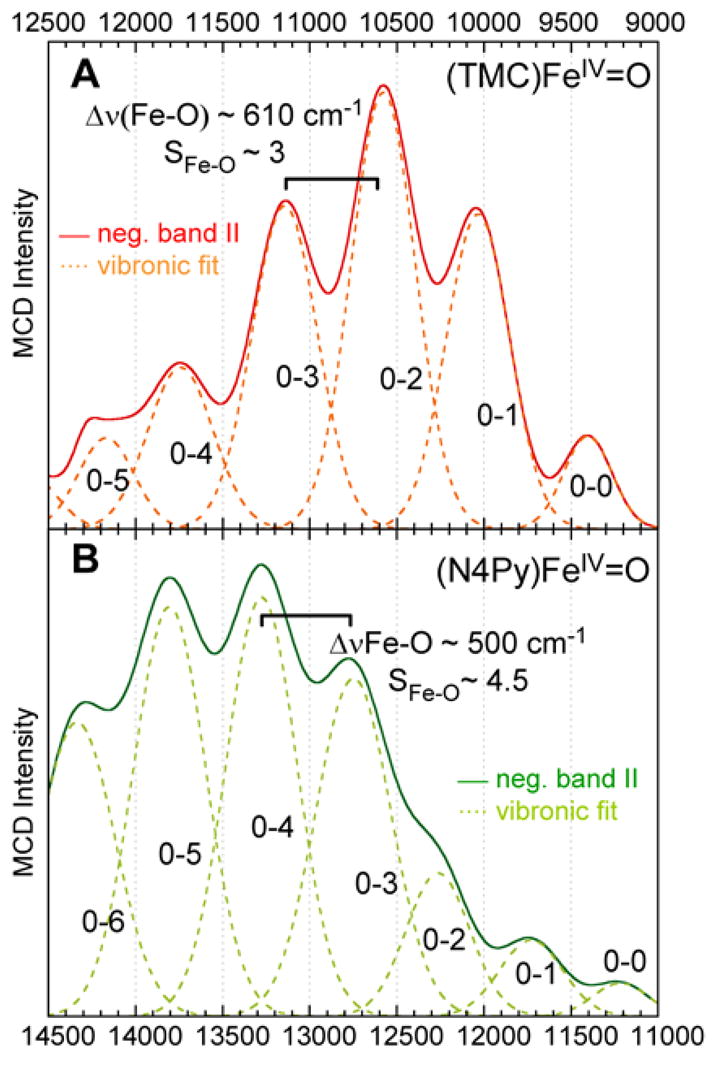
Isolated and sign-reversed band II of complexes 1 (A, solid red) and 3 (B, solid green), with individual Gaussian contributions to the vibronic progression (A, dashed orange; B, dashed light green).

$${\text{I}}_{\text{0}\to \text{n}}/{\text{I}}_{0\to 0}={({\text{S}}_{\text{Fe}-\text{O}})}^{\text{n}}/\text{n}!$$

From this equation, S_Fe-O and the measured Fe-O stretching frequency in the excited state, ν_es(Fe-O), the Energy, E_Fe-O, were established using:

$${\text{S}}_{\text{Fe}-\text{O}}={\text{E}}_{\text{Fe}-\text{O}}/v_{\text{es}}(\text{Fe}-\text{O}),$$

and the distortion in the excited state, Δr(Fe-O), was determined from

$${\text{E}}_{\text{Fe}-\text{O}}={}^1/_2\text{k}\mathrm{\Delta }\text{r}{(\text{Fe}-\text{O})}^2.$$

Table 2 presents the excited state parameters obtained through this analysis along with the ground state parameters defining the Fe-O bonding,

Table 2.

Experimental parameters for ground states and d(xy) → d(xz/yz) excited states for complexes 1 and 3.

ground state	1	3
νgs(Fe-O) [cm−1]	834 b,c	814 d
rgs(Fe-O) [Å]	1.65 b	1.64 e
Fe-O π* excited state a	1	3
νes(Fe-O) [cm−1]	610	500
SFe-O	3.0	4.5
EFe-O [cm−1]	1810	2259
Δr(Fe-O) [Å]	0.14	0.19

^aall excited state values from the MCD analysis in this study;

^bIR and x-ray data from ref.13;

^cIR data in agreement with unpublished NRVS data (ν (Fe-O) = 831 cm⁻¹) C. Bell, E.I. Solomon;

^dBell, Solomon, unpublished NRVS data;

^ex-ray data from ref. 19

The average spacing of the progression, reflecting the Fe-O stretching frequency in this d(xy) → d(xz/yz) ligand field excited state, is ν_es(Fe-O) ~ 610 cm⁻¹ and ~ 500 cm⁻¹ for complexes 1 and 3, respectively (Table 2).⁵⁹ These Fe-O stretching frequencies are considerably reduced relative to those of the ground state, ν_gs(Fe-O) = 834 cm⁻¹ and ν_gs(Fe-O) = 814 cm⁻¹ for 1 and 3 respectively. This large decrease of ~200 – 300 cm⁻¹ in ν (Fe-O) is due to an extensive weakening of the Fe-O π-bond in this excited state. The formal Fe-O bond order (BO) is reduced by ½ π-bond from BO_gs = 2 in the ground state (1 σ + 2× ½ π) to BO_es = 1.5 in this excited state (1 σ + ½ π). Thus, these direct experimental data quantitate the very strong and covalent Fe-O π-bond in these Fe^IV=O complexes. Additionally, the Fe-O bond length increases notably upon excitation, Δr(Fe-O) = 0.14 Å and 0.19 Å for complexes 1 and 3 respectively, supporting the notion that a strong Fe-O π-bond is greatly weakened and lengthened by the excitation of an electron from a nonbonding to a Fe-O π* orbital.

A comparison of complexes 1 and 3 shows similar Fe-O ground state parameters, but large differences in the excited state values (Table 2). For complex 3, the excited state Fe-O stretching frequency, ν_es(Fe-O) ~ 500 cm⁻¹, is greatly decreased compared to that of complex 1, ν_es(Fe-O) ~ 610 cm⁻¹ (see Figure 8), despite similar ground state stretching frequencies. Along with this much larger reduction in the stretching frequency, complex 3 has a much larger Huang-Rhys factor, S_Fe-O ~ 4.5 for 3 vs. S_Fe-O ~ 3.0 for 1, and thus a larger distortion of the Fe-O bond length in the excited state.

These differences in the non-bonding → π* excited state between complexes 3 and 1 directly probe the Fe-O π-bond. In contrast to the similarities in the ground state parameters, the larger reduction in stretching frequency and the larger Fe-O distortion upon excitation show that the π-contribution to the Fe-O bond in complex 3 is considerably stronger than in 1. The σ–contribution in 3 is weaker (vide infra), resulting in only a slightly lower Fe-O bond strength in the ground state of 3 relative to complex 1.

3.4 Experimental trends

Based on the detailed analysis of the vibronic structure associated with band II, the information it provides about the bonding in these complexes and the VT-MCD assignments, we can now compare the spectra of the three complexes (Figure 3 and Figure 4) and relate the differences and energy shifts to changes in the ligand field (Figure 1). Complexes 1 and 2, which both have the same equatorial TMC coordination, but different axial ligands (NCMe in 1 vs. ⁻OC(O)CF₃ in 2) will be compared first. Then complex 3 with the pentadentate N4Py ligand set, having pyridines in the equatorial plane, will be analyzed relative to complex 1.

The spectra of complex 2 relative to 1 show only slight differences, and thus the ligand field, d-orbital splitting and bonding interactions are very similar. The energy of band I is red-shifted by only ~100 cm⁻¹. This d(xy) → d(x²-y²) transition reflects the strength of the equatorial ligand field, since it excites an electron from the non-bonding d(xy) orbital into the d(x²-y²) orbital, which is σ-antibonding between the Fe and the equatorial nitrogens. Given that the equatorial ligand, TMC, is the same in both complexes, similar transition energies are expected.

The negative band II is blue-shifted by ~ 500 cm⁻¹, indicating a larger d(xy) → d(xz/yz) splitting. This larger splitting could be caused either by (1) stronger Fe-O π interactions because of a stronger, more covalent Fe-O π-bond and/or by (2) additional π* interactions between the d(xz/yz) orbitals and the anionic carboxylate ligand (⁻OC(O)CF₃) trans to the oxo. As seen in the analysis of the vibronic fine structure, the Fe-O π-bond is very similar for both complexes. Thus, the higher energy of the d(xy) → d(xz/yz) transition in 2 must reflect additional π* interactions with the axial carboxylate ligand in 2 relative to 1, where the axial ligand (NCMe) is predominantly a σ-donor.⁶⁰

Band III, the d(xz/yz) → d(x²-y²) transition, is red-shifted in 2 relative to 1 by ~ 900 cm⁻¹. This shift results from the slight decrease in energy of the d(x²-y²) orbital (slight red-shift of band I by ~100 cm⁻¹) and the destabilization of the d(xz/yz) orbitals (blue shift of band II by ~ 500 cm⁻¹) relative to the d(xy) orbital.⁶¹

The near-IR absorption spectrum of complex 2 shows a different intensity distribution of bands II and III compared to complex 1 (see section 3.1), with a more intense band II, the d(xy) → d(xz/yz) transition, and a less intense band III, the d(xz/yz) → d(x²-y²) transition. The axial carboxylate ligand results in a rhombic distortion around the iron center, which allows mixing of the d(xy) and d(xz) (in-plane with respect to the axial OCO-plane) orbitals (see section 3.5). This orbital mixing results in intensity borrowing by band II, d(xy) → d(xz/yz),from band III, d(xz/yz) → d(x²-y²). This mixing is reproduced in the DFT and TD-DFT calculations (section 3.5).

Bands IV and V can only be cleanly observed in complex 1, because of ferric impurities and an intense, low-energy LMCT band in 2. DFT calculations (see section 3.5) indicate that this LMCT transition originates from the axial carboxylate in complex 2.

To summarize: complexes 1 and 2 have the same spectral fingerprint in the lower energy region (5,000–18,000 cm⁻¹) and only minor energy shifts of these three d-d bands. These shifts are consistent with our previous assignments.²⁹ The blue shift and the decrease in absorption intensity of the d(xy) → d(xz/yz) transition in complex 2 relative to 1 reflects additional π-interactions between the iron and the axial carboxylate ligand in complex 2, which also result in the intense, low energy LMCT band in complex 2.

A comparison between the absorption and variable temperature MCD spectra of complex 3, containing the penta-coordinate N4Py ligand set, and complex 1 shows much larger changes (Figure 3). In general, a large blue-shift of at least 2,000 cm⁻¹ of all three d-d bands in the lower energy region is observed. The energy increase of these ligand field transitions reflects an increased d-orbital splitting.

Band I, the d(xy) → d(x²-y²) transition, shifts up in energy by ~3,600 cm⁻¹, indicating a much stronger equatorial ligand field in 3 compared to 1. This strong-field is caused by the pyridines, coordinated to the iron in the equatorial plane in the N4Py ligand set of 3, which are much stronger σ-donors than the tertiary amines in the equatorial TMC ligand set of 1. These stronger interactions in the equatorial plane result as well in shorter Fe-N_eq bond lengths in 3 compared to 1 (vide infra). As a result of this large blue-shift, band I is not the lowest energy transition in complex 3, in contrast to complexes 1 and 2.

The lowest energy transition in complex 3 is band II, involving an excitation from the d(xy) to the d(xz/yz) orbitals, which is shifted to higher energy relative to 1 by ~2,000 cm⁻¹. This destabilization of the d(xz/yz) orbitals could be caused either by (1) stronger Fe-O π* interactions because of a stronger, more covalent Fe-O π-bond and/or by (2) additional π* interactions between the d(xz/yz) orbitals and the equatorial pyridines.⁶² Each of the four equatorial pyridines in the N4Py ligand has delocalized π-orbitals perpendicular to the plane of the ring, which gain some overlap with the iron d(xz/yz) orbitals due to a tilt of the rings (2 × 24º and 2 × 12º according to the x-ray structure of complex 3).¹⁹ These additional Py π – d(xz/yz) interactions cause part of this destabilization. However, as seen in the vibronic fine structure analysis (section 3.3), complex 3 has a stronger and more covalent Fe-O π-bond than complex 1. Thus, the stronger Fe-O π* interactions with the oxo p(x/y) orbitals in 3 also lead to the higher energy of the d(xy) → d(xz/yz) transition.

As a result of changes in the d(xz/yz) and d(x²-y²) orbital energies discussed above, band III, the d(xz/yz) → d(x²-y²) transition, is shifted up in energy by ~2,200 cm⁻¹ in complex 3 relative to 1. This blue shift demonstrates that the d(x²-y²) orbital is destabilized more than the d(xz/yz) orbitals in complex 3 compared to 1. The near-IR absorption intensities for complexes 1 and 3 are comparable.

At higher energies (>~20,000 cm⁻¹) there are big differences between the MCD spectra of complexes 1 and 3. At ~ 24,900 cm⁻¹, the MCD spectrum of complex 1 shows the highest energy d-d band, the d(xy) → d(z²) transition. It is z-polarized, has a positive MCD signal and a relatively low absorption coefficient in the UV/Vis spectrum. In contrast, complex 3 shows a very intense, z-polarized, but negative MCD band at ~25,000 cm⁻¹ which has fine structure with an equidistant spacing, ν_ex(Fe-O) ~ 500 cm⁻¹, equivalent to band II reflecting the loss of half an Fe-O π-bond (from the vibronic analysis in section 3.3).

Several possibilities were considered for the assignment of this band. It cannot be the highest energy d-d transition, d(xy) → d(z²), because of its high absorption intensity. In addition, the reduction in stretching frequency is consistent with the loss of half a π-bond, but not of half the σ-bond. An assignment as the oxo-to-iron LMCT transition, O p(x/y) → Fe d(xz/yz), is also incompatible with the data. Excitation of an electron out of the Fe-O π-bonding and into the Fe-O π* orbital would weaken the Fe-O interaction by 2 × 1/2 π-bond, resulting in a greater decrease of Fe-O excited state stretching frequency than observed here.

The data, however, are consistent with an assignment as the z-polarized LMCT transition from the pyridine π MOs into the Fe-O π* orbitals, Py π → d(xz/yz) CT. Because of the tilt of the pyridine rings (2 × 24º and 2 × 12º according to the x-ray structure of complex 3),¹⁹ the Py π-orbitals overlap with the iron d(xz/yz) orbitals resulting in absorption and MCD intensity. For this assignment, as in band II (d(xy) → d(xz/yz)) one electron is transferred from an Fe-O non-bonding orbital, Py π, into the Fe-O π* orbitals, d(xz/yz), resulting in a vibronic excitation and a weakening the Fe-O interactions by ½ π-bond. The same vibrational frequency, ν_ex(Fe-O) ~ 500 cm⁻¹, of the Fe-O stretching mode is observed in this charge transfer excited state.

In summary the differences in the spectra between complexes 1 and 3 reflect (1) a stronger equatorial, σ-donating ligand field in 3, which shifts band I up in energy, and (2) a large increase in the strength and covalency of the Fe=O π-bond, which increases the transition energy of band II, decreases the Fe-O stretching frequency and increases the Fe-O bond length in the excited state. Further insight into these experimental electronic structure experiments is obtained through DFT calculations.

3.5 Density Functional Calculations

In order to gain further insight into the electronic structure and bonding of these Fe^IV=O complexes and to evaluate computational methods, we have carried out density functional (DFT) calculations using both the Gaussian and ADF program packages on complexes 1, 2 and 3 (for details see computational methodology).⁶³

3.5.1 Ground state parameters

A comparison of the ground state (gs) parameters (Table 3) shows good agreement between experimental data and the calculated parameters. The Fe-O bond lengths of complexes 1, 2 and 3 are the same within the error of the x-ray structures, r(Fe-O)~1.65 Å, and the computed values, r_comp.(Fe-O)=1.66–1.67Å, are very similar. The largest experimental difference between the complexes is in the equatorial ligand field, with long r(Fe-N_eq) ~2.1 Å bond lengths for the two TMC complexes (1 and 2) and a much shorter r(Fe-N_eq) ~ 1.9 Å for complex 3 with the N4Py ligand. This difference is well reproduced in the calculations. The experimental Fe-O stretching frequencies for complexes 1 and 3 show a lower frequency for 3 (ν_exp(Fe-O)=814 cm⁻¹ vs. 834 cm⁻¹) and agree well with the computed frequencies (ν_comp(Fe-O)=829 cm⁻¹ vs. 846 cm⁻¹).

Table 3.

Comparison of experimental and computational gs parameters for 1, 2, and 3:

	1		2		3
	Exp.a	Comp.b	Exp.c	Comp.b	Exp.d	Comp.b
r(Fe-O)	1.646(3)	1.655	1.64(2)	1.671	1.639(5)	1.666
r(Fe-Lax)	2.058(3)	2.12		1.98	2.033(8)	2.07
r(Fe-Neq)	2.067(3)-2.117(3)	2.13	} 2.08(2)	2.13	1.949(5)-1.964(5)	1.97
ν (Fe-O)	834e	846	--	817	814f	829

All bond length in Å, frequencies in cm⁻¹;

^afrom ref. 13;

^bcomputational results from G03/BP86/tzall (for details see methodology section 2.4);

^cEXAFS data, unpublished results, J.-U. Rohde, L. Que, Jr.;

^dfrom ref 19;

^efrom IR data, in agreement with unpublished NRVS data (ν (Fe-O) = 831 cm⁻¹) C. Bell, E.I. Solomon;

^ffrom NRVS data, unpublished results, C. Bell, E.I. Solomon.

Experimentally, all three complexes have an S=1 ground state, which is reproduced in the computations. However, the splitting to the first excited spin-state, the S=2 state depends strongly on the computational method and especially the density functional/hybrid used (Table in SI). Functional/hybrid differences of up to 13 kcal/mol in the relative energies of the spin states were calculated for the complexes. Several previous studies, especially on spin-cross-over complexes, have established that while pure density functional methods, like BP86, overly stabilize low-spin states, the hybrid functional B3LYP in general favors high-spin states.^64–68 Thus, the actual energy difference between the S=1 and S=2 states likely lies somewhere in between the calculated values. Because of this uncertainty, we only analyze the general trends over this series of compounds, which are functional independent. The spin-state splitting is similar for complexes 1 and 2, which have the same ligand in the equatorial plane, but is much larger in 3, due to its stronger equatorial ligand field.

3.5.2 Excited state parameters

In addition to the ground state parameters, we have calculated excited state parameters to compare to spectroscopy and evaluate the computational methods. We use time-dependent density functional theory (TD-DFT) as implemented in Gaussian, as well as ΔSCF in ADF to calculate energies and absorption intensities (TD-DFT only) of the electronic transitions in both the ligand-field and charge-transfer (CT) region and to obtain excited state geometries.(ADF only).

A comparison of the transition energies shows reasonable qualitative agreement between the experimental values (obtained by MCD spectroscopy) and the ones calculated by DFT (Figure 9 and Table 4).

Figure 9.

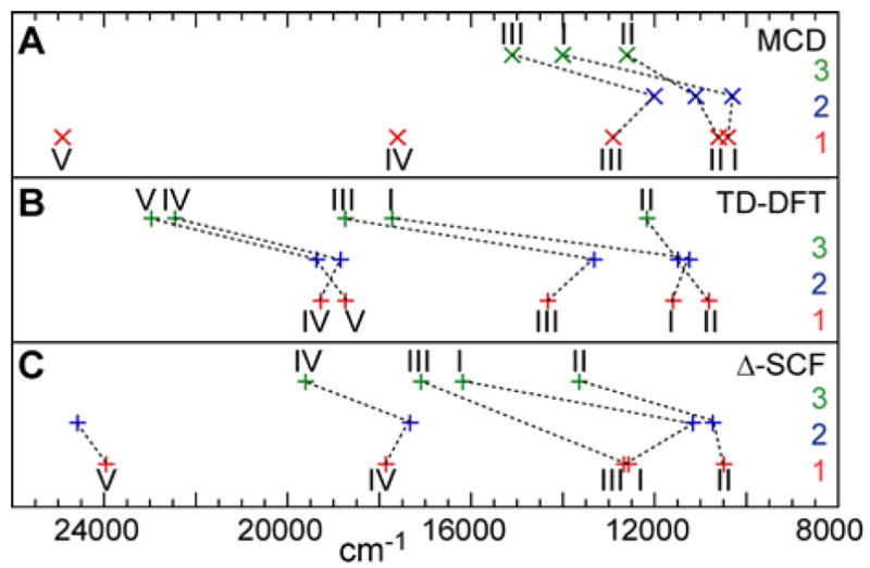
Transition energies of ligand field bands of complexes 1 (red), 2 (blue) and 3 (green) according to (A) MCD spectroscopy, (B) TD-DFT calculations and (C) ΔSCF calculations. (Missing data points either were not observed (MCD) or did not converge (ΔSCF))

Table 4.

Comparison of experimental and computational transition energies (in cm⁻¹) of complexes 1, 2, and 3.

		Experimental (MCD)			Computational (TD-DFT)a			Computational (ΔSCF)b
d-d transitions		1	2	3	1	2	3	1	2	3
I	xy → x2-y2	~10,400	~10,300	~14,000	11,594	11,238	17,718	12,570	--c	17,089
II	xy → xz/yz	~10,600	~11,100	~12,600	10,812	11,494	12,162	10,486	10,723	13,640
III	xz/yz → x2-y2	~12,900	~12,000	~15,100	14,327	13,320	18,745	12,668	11,168	16,180
IV	xz/yz → z2	~17,600	--	--	19,276	18,832	22,454	17,848	17,330	19,600
V	xy → z2	~24,900	--	--	18,733	19,364	22,961	23,948	24,577	--c

all values in cm⁻¹;

^ausing G03/BP86/tzall/solv, average given for transitions into and out of d(xz/yz);

^busing ADF/B88P86/tzall;

^cwave function not converged.

While the absolute energy values are overestimated in most cases for both the TD-DFT and ΔSCF computations by up to ~ 2000 cm⁻¹ and the energy order of transitions changes in some instances, the relative energies and trends between the complexes as discussed in section 3.4 are reproduced very well by both computational methods. Complexes 1 and 2 have similar transition energies. In 2 compared to 1 bands I and III are a red-shifted by only 100 cm⁻¹ and 900 cm⁻¹ respectively, while band II moved to slightly higher energies (by 500 cm⁻¹). The main shift, the energy of band III due to the axial ligand, is well reproduced in the calculations. All ligand field transitions of complex 3 are blue-shifted compared to 1, which is consistent with the experimental data. The lowest energy band in 3, in experiment and calculations, is band II not band I as in complex 1. The largest energy increase of 3,600 cm⁻¹ is calculated for band I, as discussed in section 3.4, which is due to the stronger equatorial ligand field in complex 3.

The relative intensities of the near-IR absorption bands are reproduced well in the TD-DFT calculations (Figure 10 and Table in SI). The calculations are consistent with the experimental assignment that the absorption intensity is associated with the ligand field transition of an electron from the d(xz) and d(yz) orbitals into the d(x² –y²) orbital (band III). Two transitions, one with the d(xz) and the other with the d(yz) orbitals as donors, are calculated to have dominant absorption intensity in this region (dashed lines in Figure 10B).⁶⁹

Figure 10.

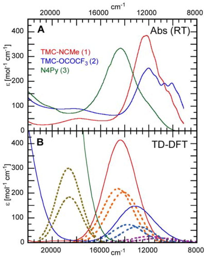
Near-IR absorption spectra for complexes 1 (red), 2 (blue) and 3 (green). (A) Experimental spectra taken at room temperature and (B) calculated TD-DFT spectra (for details see section 2.4). Solid lines: complete spectra; dashed lines: contributions of the d(xz/yz) → d(x²-y²) transitions (additionally for 2 the d(xy) → d(xz/yz) transition has intensity and is given in purple).

Reproducing the experimental spectra, the calculations show that the absorption band of complex 2 shifts to lower energy (by ~1,000 cm⁻¹) and loses overall intensity compared to 1. In addition, a second transition, from the d(xy) to the d(xz/yz) orbitals, gains intensity on the low energy shoulder of the absorption band (purple dashed lines). This corresponds to the increased fine structure observed in the experimental absorption spectrum (Figure 3A at ~ 10,000 cm⁻¹). Thus, the calculations are consistent with the analysis of section 3.4 involving orbital mixing and intensity redistribution in 2 due to the rhombic distortion associated with the orientation of the axial carboxylate ligand.

In the calculated absorption spectrum of complex 3 the Gaussians are again associated with the ligand field band III, the d(xz/yz) → d(x² –y²) transition, and show a large shift to higher energy (by ~4,400 cm⁻¹) as observed in the experimental spectra and explained by the stronger equatorial ligand field in 3.⁷⁰

Using ADF we were able to optimize the geometry of the excited state with the electronic configuration d(xy)¹d(xz/yz)³ corresponding to band II (excitation from the d(xy) to the d(xz/yz) orbitals), modeling the excited state after geometric relaxation. We have experimentally analyzed this excited state through the vibronic fine structure (section 3.3) and could quantify the increase in Fe-O distance. We can then compare the calculated and experimentally observed Fe-O bond lengths in both the ground and excited states of complexes 1 and 3.

From Table 5, the calculations reproduce very well the experimentally observed Fe-O bond lengths in the ground state. In going to the excited state, the experimentally determined increase in Fe-O bond lengths are Δr(Fe-O) = +0.14 Å and +0.19 Å for complexes 1 and 3, respectively. While this increase in Fe-O distance upon excitation is quantitatively not reproduced by the computations (Δr(Fe-O) = +0.05 Å and +0.08 Å for complexes 1 and 3, respectively), the trend of an increase in the Fe-O bond length and of a larger distortion in 3 relative to 1 in the excited states is reproduced. This stands in contrast to the similar bond lengths for 1 and 3 in the ground state and reflects the larger π contribution to the Fe-O bond in complex 3 compared to 1.

Table 5.

Comparison of experimental and calculated Fe-O bond lengths in the ground state and d(xy) → d(xz/yz) excited state for complexes 1 and 3.

	1		3
r(Fe-O) [Å]	experimental	computationala	experimental	computationala
ground state	1.65	1.65	1.64	1.65
excited state	1.79	1.70	1.83	1.73
Δr(Fe-O) [Å]	+0.14	+0.05	+0.19	+0.08

^afrom ADF/B88P86/tzp calculations, for details see methodology section 2.4.

3.5.3 Electronic structures and trends in bonding

Having established that the calculations reproduce the experimental data reasonably well, the calculated electronic structures of complexes 1 and 3 (for 2 see SI) will be analyzed with regard to their similarities and differences, focusing especially on the Fe-O bonding and correlation to experiment (section 3.4).⁷¹ Figure 11 shows the spin unrestricted energy level diagrams and relevant molecular orbitals of complexes 1 and 3, while Table 6 summarizes the electronic structure parameters.

Figure 11.

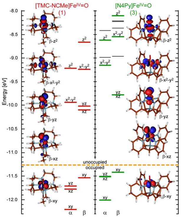
Energy level diagram and Fe-d based molecular orbitals of complexes 1 and 3 (from G03/BP86/tzall calculations, for details see methodology section 2.4). Levels in black are Py π based and not involved in Fe-O bonding.

Table 6.

Electronic structure parameters for complexes 1 and 3.

	[FeIV(O)(TMC)(NCMe)]2+ (1)			[FeIV(O)(N4Py)]2+ (3)
	Fe	O	TMC+ax	Fe	O	N4Py
spin densities	1.32	0.74	−0.06	1.24	0.83	−0.07
charges	1.35	−0.41	1.07	1.28	−0.41	1.12
alpha - MO [%]
z2	54	24	21	53	22	25
x2-y2	58	0	42	59	0	41
beta - MO [%]
Z2	56	24	19	55	21	23
x2-y2	67	0	33	58	0	42
yz	55	34	10	52	40	8
xz	54	35	11	53	39	8
bond orders	Fe--O	Fe--TMC+ax		Fe--O	Fe--N4Py
σ + π	1.66	1.97		1.60	2.52
σ	0.83	1.75		0.72	2.26
π	0.83	0.22		0.87	0.24

from G03/BP86/tzall calculations, MO% given for unoccupied orbitals, bond orders calculated using PyMOlyze⁵³

Complexes 1 and 3 have qualitatively the same electronic structure and bonding scheme. The Fe^IV=O (S=1) is a d⁴ system with a (xy)²(xz/yz)² ground configuration (Figure 1 and Figure 11). The half occupied iron d(xz/yz) orbitals form strong, covalent π-bonds with the oxo unit with large oxygen p(x/y) character in these iron d-orbitals (> 30% according to DFT calculations)²⁹ resulting in a localization of the spin on the iron–oxo unit.^72–74 The unoccupied iron d(z²) orbital forms a strong Fe–O σ-bond with the oxygen p(z). The electronic structures of both 1 and 3 are dominated by these very strong and covalent Fe–O bonding interactions.

However, differences exist between complexes 1 and 3. In complex 3, the whole d-manifold is shifted to higher energies relative to complex 1, best observed in the energies of the non-bonding d(xy) orbitals, which shift by ~ 0.2 eV (Figure 11). The iron core has a higher negative charge and the formally neutral ligands, TMC+NCMe and N4Py respectively, are more positive in 3 compared to 1 (Table 6), both effects are a result of greater equatorial ligand-to-metal charge donation and larger antibonding interactions in 3 compared to 1.

Complex 3 also has in general a larger d-orbital splitting, indicating stronger antibonding interactions between the iron and the equatorial ligands. Experimentally, this can be observed in the higher energy of the ligand field transitions, bands I and II in particular.

A more detailed analysis of the orbital interactions gives specific bonding contributions. In the equatorial plane, the pyridines in the N4Py ligand set (3) are stronger σ-donors compared to the amines in TMC (1). This is reflected by the larger ligand- and decreased Fe-contributions to the d(x²-y²) orbital in 3 compared to 1 (β-spin: +9% N4Py, −9% Fe). The more covalent bonding interactions in the equatorial plane account for some of the additional charge donation to the iron center. The N4Py σ-donor orbitals also interact with the Fe d(z²) orbital, reflected by larger ligand contributions in 3 compared to 1 (~ +4% N4Py, Table 6). Thus, the d(z²) orbital is destabilized more in 3 compared to 1 (relative to the non-bonding d(xy) orbitals, Figure 11) due to these stronger σ-antibonding interactions with N4Py. Both these orbital interactions (between the N4Py ligand and the Fe d(x²-y²) and d(z²) orbitals) together are reflected in the bond-order-analysis (BOA)⁷⁵ (Table 6) with stronger, Fe -- N4Py than Fe -- TMC+NCMe bonding interactions (2.52 vs. 1.97). Experimentally, the strong σ-donor character of the N4Py ligand set is indicated by the much shorter Fe-N_eq distances (Table 3) and the higher energy of band I, the d(xy) → d(x²-y²) transition (section 3.4).

In contrast to the stronger Fe-N4Py σ-bonds, the Fe-O σ-interactions are weaker in 3 compared to 1. Indications for this weaker Fe-O σ-bond are the smaller oxo contributions (~−3%) in the d(z²) orbitals oxo in 3 compared to 1 and the smaller σ-bonding contribution to the Fe-O bond order (0.83 in 1 vs. 0.72 in 3).

Alternatively, the π-contribution to the Fe-O bond is stronger in 3 compared to 1. The calculations reproduce the experimental trends from section 3.3. These stronger, more covalent Fe-O π-interactions result in larger oxo contributions to the d(xz/yz) orbitals in 3 compared to 1 (~ +5% oxo, Table 6) and larger spin densities on the oxo (0.74 in 1 vs 0.83 in 3 ).⁷⁶ The same trend is seen in the larger Fe-O π-bond orders (0.83 for 1 vs 0.87 for 3) and the larger energy splitting between the d(xy) and d(xz/yz) orbitals (Figure 11). Experimentally, the stronger Fe-O π-bond is observed in the higher transition energy of band II (d(xy) → d(xz/yz)) in 3 compared to 1 (Figure 3 and section 3.4), and directly in the vibrational frequencies in the vibronic progression (Figure 8 and section 3.3).

To summarize, the calculated electronic structure parameters support the experimental analysis of a stronger and more covalent Fe-O π-bond in 3 compared to 1. In addition, the calculations demonstrate a weaker σ-contribution to the Fe-O bond in 3 compared to 1. The overall Fe-O bond (both σ + π-bonding contributions) is slightly weaker in 3 compared to 1, as is reflected in the stretching frequencies (experimental and calculated, Table 3) and in the bond orders (1.66 for 1 vs. 1.60 for 3, Table 6).

3.5.4 Differences in reactivity

These differences in the experimental and calculated electronic structures and especially in the Fe-O bonding, provide insight into the differences in reactivity between complexes 1 and 3 and into the general mechanism of activation. With regard to the hydrogen-atom-abstraction reaction,

$$({\text{L}}_{\text{5}}){\text{Fe}}^{\text{IV}}=\text{O}+\text{R}-\text{H}\to {\text{(L}}_{\text{5}}{\text{)Fe}}^{\text{III}}{-\text{OH}+\text{R}}^{•}$$

the reactivities of these two complexes are extremely different. While complex 3 is very reactive, capable of cleaving the strong C-H bonds of cyclohexane (D_C-H ~ 99.3 kcal/mol),¹⁶ complex 1 is reactive only towards relative weak C-H bonds like those of dihydroanthracene (D_C-H ~ 75.3 kcal/mol).²²

To consider the thermodynamics, the reaction energies for the abstraction of a tertiary hydrogen atom from 2,3-dimethylbutane by the Fe^IV=O (S=1) complexes 1 and 3 resulting in Fe^III-OH (S=1/2) species⁷⁷ and an organic radical (S=1/2) were calculated (Table 7). While complex 1 has a fairly high Gibbs Free Reaction Energy (ΔG = +17.6 kcal/mol), the same reaction is almost thermoneutral for 3 ((ΔG = +3.9 kcal/mol). This difference of ΔΔG ~ 14 kcal/mol between complexes 1 and 3 reproduces their experimentally observed difference in reactivity.

Table 7.

Calculated energies of the H-atom abstraction reaction by Fe^IV=O complexes 1 and 3 from 2,3-dimethylbutane

	[FeIV(O)(TMC)(NCMe)]2+ (1)	[FeIV(O)(N4Py)]2+ (3)
Δε (gas)	24.2	11.3
Δε (solv)	21.5	7.7
ΔE(solv)	19.9	6.2
ΔG(solv)	17.6	3.9

all values in kcal/mol; G03/B3LYP/6-311G*, Δε without zero-point energy (ZPE), ΔE with ZPE, solvent=acetonitrile; all Fe^IV=O reactants with S=1 ground state, all Fe^III-OH products with S=1/2 ground state.

Since for both complexes the substrate is the same, the difference in reaction energy must be due to differences in the stability of the Fe^IV=O reactants and/or the Fe^III-OH products. In the Fe^IV=O reactants the Fe-O π-bond is stronger in complex 3 compared to 1, but the Fe-O σ-bond is weaker, resulting in a weaker total Fe-O bond in 3 compared to 1 (vide supra). This is reflected by the lower Fe-O stretching frequency (experimentally and computationally, Table 3) and the lower total Fe-O bond order (Table 6). In contrast, in the Fe^III-OH products the total Fe-O bond is stronger in 3 compared to 1, indicated by the calculated larger Fe-O stretching frequency and a higher Fe-O bond order (for values see table in SI).⁷⁸ Thus, 3 has a weaker Fe-O bond in the reactants and a stronger Fe-O bond in the products, relative to complex 1, which leads to its lower reaction energy.

In addition to the thermodynamic stabilization, the kinetic difference in reactivity between complex 1 and 3 was considered using Frontier-Molecular-Orbital (FMO) theory. A hydrogen-atom abstraction is an electrophilic attack by the Fe^IV=O acceptor. According to FMO-theory, a good electrophile has low-energy, unoccupied orbitals with high MO coefficients on the reacting atom to achieve good overlap with the FMO’s on the donor substrate. In the Fe^IV=O (S=1) systems, the low-lying unoccupied β-spin Fe-d(xz/yz) orbitals are the important FMO’s, interacting with the electron density of the C-H σ-bond of the substrate (Figure 12 left).^79,80 The strong and covalent Fe-O π-bond results in large oxygen character in these Fe-O π* orbitals (> 30 % according to DFT, vide supra), which makes the Fe^IV=O complexes highly electrophilic and reactive towards H-atom abstraction.

Figure 12.

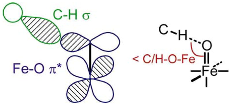
Scheme of interacting frontier molecular orbitals in the H-atom abstraction reaction (left) and optimal orientation between the Fe^IV=O complex and the substrate (right).

As we have found experimentally, complex 3 has a stronger, more covalent Fe-O π-bond (section 3.3) compared to 1 resulting in larger oxygen coefficients in the β-spin d(xz/yz) orbitals (Table 6), which are the FMO for hydrogen atom abstraction. Thus, 3 is a better electrophile and more reactive compared to 1.

Finally, in addition to large MO coefficients, good overlap between the reacting orbitals on electrophile and substrate is required. For good overlap of the C-H σ-bond with the Fe-O π* orbital, a “horizontal approach”, with a Fe-O-H/C angle of ~ 120º assures the best interaction (Figure 12 right).^80–82 However, because of the ligand sterics, the oxygen atom in complex 1 is rather sheltered by the hydrogens of the TMC ligand and buried (Figure 13 left).¹³ Thus, because of the steric hindrance of the TMC ligand in complex 1, the substrate cannot achieve an optimal orientation for good overlap with the O-p(x/y) orbitals. Alternatively, the N4Py ligand of complex 3 allows more open access to the oxygen atom (Figure 13 right) for reaction with the C-H σ-bond on the substrate.

Figure 13.

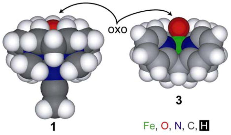
X-ray structures of complexes 1 and 3 shown as a space-filling model (CPK x 0.8, Fe is shown in green, oxygen in red, nitrogen in blue, carbon in grey and hydrogen in white).

Alkane hydroxylation reactions, including an H-atom abstraction as the first reaction step, by these Fe^IV=O model complexes have been calculated.^82,83 The results agree qualitatively with those obtained here. However, no explanation for the striking difference in reactivity between complex 1 and 3 was given.

To summarize, three contributions to the differences in the H-atom abstraction reactivity between complexes 1 and 3 are identified: (1) Considering the thermodynamics of the reaction, the weaker Fe-oxo bond in the Fe^IV=O reactant and stronger Fe-hydroxy bond in Fe^III-OH product in complex 3 compared to 1 contribute to the difference in reaction energies. (2) Because of steric restrictions in the TMC ligand of complex 1, the substrate cannot approach the oxo for optimal π-orbital overlap required for good reactivity. (3) An important contribution, developed in this study, is the strength and covalency of the Fe-O π-bond. The stronger, more covalent Fe-O π-bond in complex 3 results in higher oxo character in the important FMO for this reaction, the d(xz/yz) orbitals, and thus makes 3 a stronger electrophile than 1.

4 Discussion

The MCD spectroscopy presented in this study provides a detailed experimental description of the electronic structures of Fe^IV=O (S=1) model complexes. In particular, it directly probes the energetically low-lying unoccupied molecular orbitals, which are the key frontier molecular orbitals (FMOs) for reactivity (here electrophilic attack). The VT-MCD spectra give the polarizations of electronic transitions in frozen solution, information generally available only through single-crystal experiments. This has enabled us to assign the transition from the β-spin non-bonding d(xy) to the Fe-O π* d(xz/yz) orbitals, which are the important FMOs for electrophilic attack.

In addition, the resolved fine-structure in the MCD spectra, i.e. a vibronic progression in this nb → π* excited state, provides an experimental probe of how the properties of the Fe-O bonding change compared to the ground state. The Fe-O stretching frequency and the Fe-O bond length in the excited state give detailed information on the π-contribution to the strength and covalency of the Fe-O bond. The Fe-O stretching frequency, ν_ex(Fe-O), is found to greatly decrease and the Fe-O bond length, r_ex(Fe-O), to greatly increase in this excited state compared to the ground state, indicating that the Fe-O π-bond makes a very large contribution to the total Fe-O bond, which shifts significant oxo p(x/y) character into the Fe d(xz/yz) LUMOs, activating the Fe^IV=O for reactivity.

From the MCD data we obtain detailed electronic structure trends on the three Fe^IV=O (S=1) model complexes, [Fe^IV(O)(TMC)(NCMe)]²⁺ 1, [Fe^IV(O)(TMC)(OC(O)CF₃)]⁺ 2, and [Fe^IV(O)(N4Py)]²⁺ 3. While complexes 1 and 2 have the same spectral fingerprint in the lower energy region (5,000–18,000 cm⁻¹) and only minor energy shifts (<900 cm⁻¹) of the three d-d bands, complex 3 shows much larger changes with energy shifts >3500 cm⁻¹. The spectral differences between complexes 1 and 3 reflect (i) a stronger equatorial, σ-donating ligand field in 3 due to the N4Py ligation, and (ii) a significant increase in the strength and covalency of the Fe-O π-bond in 3 compared to 1. This is reflected in the even greater decrease in ν_ex(Fe-O) and greater increase in r_ex(Fe-O) in 3 compared to 1. This difference in the Fe-O π-bond is an important contribution to the differences in reactivity towards H-atom abstraction between complexes 1 and 3. The stronger, more covalent Fe-O π-bond in complex 3 results in higher oxo character in the important FMO for this reaction, making 3 a stronger electrophile and more reactive towards H-atom abstraction compared to complex 1.

Understanding the electronic structure in these structurally defined Fe^IV=O (S=1) model systems is an important step toward understanding biologically relevant Fe^IV=O (S=1) intermediates, for example the polypeptide antibiotic bleomycin (BLM). It is suggested that the second intermediate of this anticancer drug is an Fe^IV=O (S=1) species, capable of hydrogen-atom abstraction.⁸⁰ Its calculated electronic structure is qualitatively similar to those of the model complexes in this study, as it is also characterized by a strong and covalent Fe-O π-bond. The unoccupied β-spin Fe-O π* d(xz/yz) orbitals were identified as the key FMOs in the calculated reaction coordinate and transition state for H-atom abstraction.⁸⁰

Furthermore, we can extend these insights to the biologically relevant Fe^IV=O (S=2) intermediates in non-heme iron enzymes and the enzymatic mechanism of C-H bond cleavage. Even though the Fe^IV=O intermediates in non-heme iron enzymes are found to be high-spin (S=2),^5,9,10 a previous study using experimentally calibrated DFT calculations⁸⁴ has shown that the Fe-O bonding in the S=2 enzyme intermediates is similar to that of the S=1 species, with a similar total bond-order as well as similar σ- and π-contributions to the Fe-O bond. The reason for the similarity in Fe-O bonding is the fact that Fe^IV=O (S=2) systems with an electronic configuration of (xy)¹(xz/yz)²(x²-y²)¹ differ from the S=1 species (with a (xy)²(xz/yz)² configuration) only in a change in occupation of the d(xy) and d(x²-y²) orbitals, which are perpendicular to the Fe-O axis and not involved in Fe-O bonding.²⁹

However, there are differences possible in the reactivity between Fe^IV=O (S=1) and (S=2) systems, since the reactivity is controlled not by the bonding, occupied MOs, but by the unoccupied FMOs. Two different reaction channels were identified for Fe^IV=O (S=2) enzyme intermediates in previous studies.^81,85,86 The first also involves the unoccupied β-spin d(xz/yz) orbitals.⁸¹ This is the case for the catalytic cycle of the non-heme iron enzyme 4-hydroxymandelate synthase (HmaS), which is believed to involve a high-spin Fe^IV=O intermediate performing an H-atom abstraction reaction.⁸⁷ The calculated reaction coordinate and transition state for this reaction shows that for this S=2 intermediate, the unoccupied β-spin Fe-O π* orbitals interact with the substrate and are the FMOs involved in this enzymatic reaction mechanism.⁸¹ However, this enzyme system can be regarded as a special case, since the substrate is directly coordinated to the Fe-active site and thus sterically restricted to a horizontal approach. Nevertheless, it has shown that independent of the spin state, S=1 and S=2 Fe^IV=O complexes can use this π-FMO mechanism for H-atom abstraction.

In general, however, the Fe^IV=O S=2 species have another possible reaction pathway in addition to the interaction with the substrate through the β-spin d(xz/yz) orbitals. Because of spin-polarization, the unoccupied α-spin Fe-O σ* d(z²) orbital is stabilized to lower energies and has much more oxo character in S=2 species compared to the S=1 model complexes.^81,88 Thus, in addition to the more horizontal approach and interaction with the β-spin d(xz/yz) orbitals as in S=1 complexes and geometrically constrained S=2 systems,^81,85 a vertical orientation of the substrate and interaction with the α-spin Fe-O σ* d(z²) orbital, i.e. a σ-FMO mode, is possible for the electrophilic attack by Fe^IV=O (S=2) species in enzymatic cycles, as calculated for the non-heme iron enzyme 4-hydroxyphenylpyruvate dioxygenase (HPDD)⁸¹ and for an unconstrained substrate.⁸⁶ Thus, in the determination of σ- vs. π-reaction pathways of the Fe^IV=O (S=2) species in different enzymatic cycles an investigation of the restrictions imposed by the protein pocket is required.

It should also be noted for BLM (S=1, π-attack), HmaS (S=2, π-attack) and HPPD (S=2, σ-attack) that increasing the Fe-O distance to that of the transition state, i.e. r_TS(Fe-O)~1.76Å, leads to a polarization of the FMOs. While in one orbital the iron character increases significantly, the other orbital, which interacts with the substrate, contains little iron character, and instead dominant oxygen and substrate contributions (Figure 14). This polarization and localization reflects an increase in ferric-oxyl, Fe^III-O^.−, character of the Fe=O unit with the reduction of the Fe^IV and the oxidation of the oxo in the transition state. Localization of the oxygen character in one of the LUMOs further activates the Fe-O bond at the transition state and contributes to the reactivity.⁸¹

Figure 14.

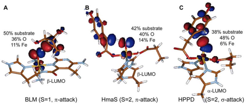
Key molecular orbital at the transition state of an electrophilic reaction by Fe^IV=O species. (A) The anticancer drug bleomycin (BLM) (S=1, π-attack) from ref.80. The enzyme intermediates of (B) HmaS (S=2, π-attack) and (C) HPPD (S=2, σ-attack) from ref.81

To summarize, through the VT-MCD spectroscopy and the resolved vibronic fine structure we are able to directly probe the frontier molecular orbitals involved in the reactivity of Fe^IV=O (S=1) model complexes. A correlation of the differences among the spectra and electronic structures of the Fe-O model complexes reveals that the strength, hence covalency, of the Fe-O π-bond makes an important contribution to reactivity. An extension to biologically relevant Fe^IV=O (S=1) and (S=2) systems shows that these can perform electrophilic attack reactions along the same π-FMO pathway, but also have an additional reaction channel (σ-FMO pathway) for the Fe^IV=O (S=2) intermediates.

Supplementary Material

SI1. Supporting Information Available.

Details on the experimental analysis, complete reference ³⁶, tables including more computational data and the cartesian coordinates of all optimized structures. This material is available free of charge via the internet at http://pubs.acs.org.

References

- 1.Solomon EI, Brunold TC, Davis MI, Kemsley JN, Lee SK, Lehnert N, Neese F, Skulan AJ, Yang YS, Zhou J. Chem Rev. 2000;100:235–349. doi: 10.1021/cr9900275. [DOI] [PubMed] [Google Scholar]
- 2.Costas M, Mehn MP, Jensen MP, Que L., Jr Chem Rev. 2004;104:939–986. doi: 10.1021/cr020628n. [DOI] [PubMed] [Google Scholar]
- 3.Sono M, Roach MP, Coulter ED, Dawson JH. Chem Rev. 1996;96:2841–2887. doi: 10.1021/cr9500500. [DOI] [PubMed] [Google Scholar]
- 4.Ferguson-Miller S, Babcock GT. Chem Rev. 1996;96:2889–2907. doi: 10.1021/cr950051s. [DOI] [PubMed] [Google Scholar]
- 5.Price JC, Barr EW, Tirupati B, Bollinger JM, Krebs C. Biochemistry. 2003;42:7497–7508. doi: 10.1021/bi030011f. [DOI] [PubMed] [Google Scholar]
- 6.Price JC, Barr EW, Glass TE, Krebs C, Bollinger JM. J Am Chem Soc. 2003;125:13008–13009. doi: 10.1021/ja037400h. [DOI] [PubMed] [Google Scholar]
- 7.Proshlyakov DA, Henshaw TF, Monterosso GR, Ryle MJ, Hausinger RP. J Am Chem Soc. 2004;126:1022–1023. doi: 10.1021/ja039113j. [DOI] [PubMed] [Google Scholar]
- 8.Riggs-Gelasco PJ, Price JC, Guyer RB, Brehm JH, Barr EW, Bollinger JM, Krebs C. J Am Chem Soc. 2004;126:8108–8109. doi: 10.1021/ja048255q. [DOI] [PubMed] [Google Scholar]
- 9.Hoffart LM, Barr EW, Guyer RB, Bollinger JM, Krebs C. Proc Natl Acad Sci USA. 2006;103:14738–14743. doi: 10.1073/pnas.0604005103. [DOI] [PMC free article] [PubMed] [Google Scholar]
- 10.Galonic DP, Barr EW, Walsh CT, Bollinger JM, Krebs C. Nature Chem Biol. 2007;3:113–116. doi: 10.1038/nchembio856. [DOI] [PubMed] [Google Scholar]
- 11.Sinnecker SSN, Barr EW, Ye S, Bollinger JM, Jr, Neese F, Krebs C. J Am Chem Soc. 2007;129:6168–6179. doi: 10.1021/ja067899q. [DOI] [PubMed] [Google Scholar]
- 12.Grapperhaus CA, Mienert B, Bill E, Weyhermuller T, Wieghardt K. Inorg Chem. 2000;39:5306–5317. doi: 10.1021/ic0005238. [DOI] [PubMed] [Google Scholar]
- 13.Rohde JU, In JH, Lim MH, Brennessel WW, Bukowski MR, Stubna A, Münck E, Nam W, Que L., Jr Science. 2003;299:1037–1039. doi: 10.1126/science.299.5609.1037. [DOI] [PubMed] [Google Scholar]
- 14.Lim MH, Rohde JU, Stubna A, Bukowski MR, Costas M, Ho RYN, Münck E, Nam W, Que L., Jr Proc Natl Acad Sci USA. 2003;100:3665–3670. doi: 10.1073/pnas.0636830100. [DOI] [PMC free article] [PubMed] [Google Scholar]
- 16.Kaizer J, Klinker EJ, Oh NY, Rohde JU, Song WJ, Stubna A, Kim J, Münck E, Nam W, Que L., Jr J Am Chem Soc. 2004;126:472–473. doi: 10.1021/ja037288n. [DOI] [PubMed] [Google Scholar]
- 17.Balland V, Charlot MF, Banse F, Girerd JJ, Mattioli TA, Bill E, Bartoli JF, Battioni P, Mansuy D. Eur J Inorg Chem. 2004:301–308. [Google Scholar]
- 18.Martinho M, Banse F, Bartoli JF, Mattioli TA, Battioni P, Horner O, Bourcier S, Girerd JJ. Inorg Chem. 2005;44:9592–9596. doi: 10.1021/ic051213y. [DOI] [PubMed] [Google Scholar]
- 19.Klinker EJ, Kaizer J, Brennessel WW, Woodrum NL, Cramer CJ, Que L., Jr Angew Chem Int Ed. 2005;44:3690–3694. doi: 10.1002/anie.200500485. [DOI] [PubMed] [Google Scholar]
- 20.Bukowski MR, Koehntop KD, Stubna A, Bominaar EL, Halfen JA, Münck E, Nam W, Que L., Jr Science. 2005;310:1000–1002. doi: 10.1126/science.1119092. [DOI] [PubMed] [Google Scholar]
- 21.Jensen MP, Costas M, Ho RYN, Kaizer J, Payeras AMI, Münck E, Que L, Jr, Rohde J-U, Stubna A. J Am Chem Soc. 2005;127:10512–10525. doi: 10.1021/ja0438765. [DOI] [PubMed] [Google Scholar]
- 22.Rohde JU, Que L., Jr Angew Chem Int Ed. 2005;44:2255–2258. doi: 10.1002/anie.200462631. [DOI] [PubMed] [Google Scholar]
- 23.Sastri CV, Park MJ, Ohta T, Jackson TA, Stubna A, Seo MS, Lee J, Kim J, Kitagawa T, Münck E, Que L, Jr, Nam W. J Am Chem Soc. 2005;127:12494–12495. doi: 10.1021/ja0540573. [DOI] [PubMed] [Google Scholar]
- 24.Sastri CV, Seo MS, Park MJ, Kim KM, Nam W. Chem Commun. 2005:1405–1407. doi: 10.1039/b415507f. [DOI] [PubMed] [Google Scholar]
- 25.Bautz J, Bukowski MR, Kerscher M, Stubna A, Comba P, Lienke A, Münck E, Que L., Jr Angew Chem Int Ed. 2006;45:5681–5684. doi: 10.1002/anie.200601134. [DOI] [PubMed] [Google Scholar]
- 26.Pestovsky O, Stoian S, Bominaar EL, Shan XP, Münck E, Que L, Jr, Bakac A. Angew Chem Int Ed. 2005;44:6871–6874. doi: 10.1002/anie.200502686. [DOI] [PubMed] [Google Scholar]
- 27.Pestovsky O, Stoian S, Bominaar EL, Shan X, Münck E, Que L, Jr, Bakac A. Angew Chem Int Ed. 2006;45:340. [Google Scholar]
- 28.Lehnert N, Ho RYN, Que L, Jr, Solomon EI. J Am Chem Soc. 2001;123:8271–8290. doi: 10.1021/ja010165n. [DOI] [PubMed] [Google Scholar]
- 29.Decker A, Rohde J-U, Que L, Jr, Solomon EI. J Am Chem Soc. 2004;126:5378–5379. doi: 10.1021/ja0498033. [DOI] [PubMed] [Google Scholar]
- 30.Neese F. J Inorg Biochem. 2006;100:716–726. doi: 10.1016/j.jinorgbio.2006.01.020. [DOI] [PubMed] [Google Scholar]
- 31.Schoneboom JC, Neese F, Thiel W. J Am Chem Soc. 2005;127:5840–5853. doi: 10.1021/ja0424732. [DOI] [PubMed] [Google Scholar]
- 32.where “TMC” is 1,4,8,11-tetramethyl-11,14,18,11-tetraazacyclotetradecane.
- 33.where “N4Py” is N, N-bis(2-pyridylmethyl)-N-bis(2-pyridyl)methylamine.
- 34.Armarego WLF, Perrin DD. Purification of Laboratory Chemicals. 4. Pergamon Press; Oxford: 1997. [Google Scholar]
- 35.Lubben M, Meetsma A, Wilkinson EC, Feringa B, Que L., Jr Angew Chem Int Ed. 1995;34:1512–1514. [Google Scholar]
- 36.Frisch MC, et al. Gaussian 03, Revision C02. Gaussian, Inc; Wallingford CT: 2004. for complete reference see Supporting Information. [Google Scholar]
- 37.ADF2003.01. Theoretical ChemistryVrije Universiteit; Amsterdam, The Netherlands: SCM. http://www.scm.com. [Google Scholar]
- 38.Fonseca Guerra C, Snijders JG, te Velde G, Baerends EJ. Theor Chem Acc. 1998;99:391. [Google Scholar]
- 39.te Velde G, Bickelhaupt FM, van Gisbergen SJA, Fonseca Guerra C, Baerends EJ, Snijders JG, Ziegler T. J Comput Chem. 2001;22:931–967. [Google Scholar]
- 40.Vosko S, Wilk L, Nusair M. Can J Phys. 1980;58:1200–1211. [Google Scholar]
- 41.Becke AD. Phys Rev A. 1988;38:3098–3100. doi: 10.1103/physreva.38.3098. [DOI] [PubMed] [Google Scholar]
- 42.Perdew JP. Phys Rev B. 1986;33:8822–8824. doi: 10.1103/physrevb.33.8822. [DOI] [PubMed] [Google Scholar]
- 43.Becke AD. Chem Phys. 1986;84:4524–4529. [Google Scholar]
- 44.Perdew JP, Zunger A. Phys Rev B. 1981;23:5048. [Google Scholar]
- 45.Becke AD. J Chem Phys. 1993;98:5648–5652. [Google Scholar]
- 46.Dunning TH, Jr, Hay PJ. In: Modern Theoretical Chemistry. Schaefer HF III, editor. Plenum; New York: 1976. [Google Scholar]
- 47.Hay PJ, Wadt WR. J Chem Phys. 1985;82:270–283. [Google Scholar]
- 48.Hay PJ, Wadt WR. J Chem Phys. 1985;82:299–310. [Google Scholar]
- 49.Wadt WR, Hay PJ. J Chem Phys. 1985;82:284–298. [Google Scholar]
- 50.Miertus S, Scrocco E, Tomasi J. Chem Phys. 1981;55:117. [Google Scholar]
- 51.Miertus S, Tomasi J. Chem Phys. 1982;65:239. [Google Scholar]
- 52.Cossi M, Barone V, Cammi R, Tomasi J. Chem Phys Lett. 1996;255:327. [Google Scholar]
- 53.Tenderholt AL. PyMOlyze, Version 2.0. Stanford University; Stanford, CA, USA: http://pymolyze.sourceforge.net. [Google Scholar]
- 54.Schaftenaar G, Noordik JH. J Comput-Aided Mol Design. 2000;14:123–134. doi: 10.1023/a:1008193805436. http://www.cmbi.ru.nl/molden/molden.html. [DOI] [PubMed]
- 55.gOpenMol, CSC; http://www.csc.fi/gopenmol/.
- 56.These features vary in intensity with samples and preparations, their intensity was minimal in samples with highest purity. They are likely due to ferric impurities. Ferrous species do not contribute to the MCD signal in this energy region and iron-dimer species will not be paramagnetic at these low temperatures.
- 57.unpublished results for complex 2, L. Que, Jr.
- 58.Gaussian fits of bands I and III were subtracted from the MCD spectra to isolate band II and the sign was reversed (neg. to pos.). The MCD spectra of all measured temperatures were analyzed and the reported values are averages over all temperatures. Detailed analyis for complex 2 is more challenging due to strongly overlapping bands, and thus was carried out only for complexes 1 and 3.
- 59.It was possible to measure the excited state frequency of complex 2 (νes(Fe-O)~620 cm−1), which is very similar to that of complex 1.
- 60.The π-backbonding interaction from the NCMe ligand is very weak in the high-valent FeIV=O complex (vide infra).
- 61.The shifts in energy between these three transitions are not quantitative because the one-electron orbital energies do not allow for electronic relaxation. Differences in covalency of the orbitals involved in the transitions are taken into account.
- 62.The axial tertiary amine in the N4Py ligand-set trans to the oxo is a σ-donor only and thus cannot interact with the d(xz/yz) orbitals.
- 63.We mainly present results from Gaussian 03 calculations with the BP86 functional. The other programs/methods/functionals give qualitatively the same results and can be found in the Supporting Information.
- 64.Paulsen H, Duelund L, Winkler H, Toftlund H, Trautwein HX. Inorg Chem. 2001;40:2201–2203. doi: 10.1021/ic000954q. [DOI] [PubMed] [Google Scholar]
- 65.Salomon O, Reiher M, Hess BA. J Chem Phys. 2002;117:4729–4737. [Google Scholar]
- 66.Reiher M. Inorg Chem. 2002;41:6928–6935. doi: 10.1021/ic025891l. [DOI] [PubMed] [Google Scholar]
- 67.Vargas A, Zerara M, Krausz E, Hauser A, Daku LML. J Chem Theory Comput. 2006;2:1342–1359. doi: 10.1021/ct6001384. [DOI] [PubMed] [Google Scholar]
- 68.Herrmann C, Yu L, Reiher M. J Comput Chem. 2006;27:1223–1239. doi: 10.1002/jcc.20409. [DOI] [PubMed] [Google Scholar]
- 69.Since the complex is not strictly C4v, the d(xz) and d(yz) orbitals are not degenerate, causing the electronic transitions into and out of this orbital pair to be slightly split in energy.
- 70.The calculated intensities do not agree with the experimental trend (i.e. lower intensity in 3 compared to 1), because intense MLCT transitions calculated at similar energies, but not present experimentally, are mixed into this d-d transition.
- 71.We present results from Gaussian calculations with the pure density functional BP86, but the hybrid functional B83LYP or the ADF program with the B88P86 functional give qualitatively the same results and are given in SI.
- 72.Ghosh A, Almlof J, Que L. J Phys Chem. 1994;98:5576–5579. [Google Scholar]
- 73.Kuramochi H, Noodleman L, Case DA. J Am Chem Soc. 1997;119:11442–11451. [Google Scholar]
- 74.Decker A, Solomon EI. Angew Chem Int Ed. 2005;44:2252–2255. doi: 10.1002/anie.200462182. [DOI] [PubMed] [Google Scholar]
- 75.BOA according to Mayer’s Bond Orders, for details see implementation in PyMOlyze [Tenderholt, A. L., PyMOlyze, Version 2.0. Stanford University, Stanford, CA, USA. http://pymolyze.sourceforge.net.].
- 76.The spin densities are a direct reflection of the contributions in the ½ occupied d(xz/yz) orbitals (occupied in α-spin, unoccupied in β-spin).
- 77.For both FeIII-OH complexes the low-spin state (S=1/2) is calculated to be the ground state, with the S=5/2 state higher in energy (see SI) in agreement with experimental data on the (N4Py)FeIII-OH complex. [ Roelfes, et al. Inorg Chem. 1999;19(38):1929–1936. doi: 10.1021/ic980983p.].
- 78.The main contribution to this difference is the Fe-O π-bond strength. According to DFT calculations, the σ-donor interactions of the acetonitrile with the iron, which are competing with the Fe-O bond, are stronger in the Fe(III)-OH compared to the Fe(IV)=O complex, thus weakening the Fe-O bond more in 1 compared to 3.
- 79.Decker A, Solomon EI. Curr Opin Chem Biol. 2005;9:152–163. doi: 10.1016/j.cbpa.2005.02.012. [DOI] [PubMed] [Google Scholar]
- 80.Decker A, Chow MS, Kemsley JN, Lehnert N, Solomon EI. J Am Chem Soc. 2006;128:4719–4733. doi: 10.1021/ja057378n. [DOI] [PubMed] [Google Scholar]
- 81.Neidig ML, Decker A, Choroba OW, Huang F, Kavana M, Moran GR, Spencer JB, Solomon EI. Proc Natl Acad Sci USA. 2006;103:12966–12973. doi: 10.1073/pnas.0605067103. [DOI] [PMC free article] [PubMed] [Google Scholar]
- 82.Hirao H, Kumar D, Que L, Shaik S. J Am Chem Soc. 2006;128:8590–8606. doi: 10.1021/ja061609o. [DOI] [PubMed] [Google Scholar]
- 83.Kumar D, Hirao H, Que L, Shaik S. J Am Chem Soc. 2005;127:8026–8027. doi: 10.1021/ja0512428. [DOI] [PubMed] [Google Scholar]
- 84.Decker A, Clay MD, Solomon EI. J Inorg Biochem. 2006;100:697–706. doi: 10.1016/j.jinorgbio.2006.01.013. [DOI] [PubMed] [Google Scholar]
- 85.Borowski T, Bassan A, Siegbahn PEM. Biochemistry. 2004;43:12331–12342. doi: 10.1021/bi049503y. [DOI] [PubMed] [Google Scholar]
- 86.de Visser SP. J Am Chem Soc. 2006;128:9813–9824. doi: 10.1021/ja061581g. [DOI] [PubMed] [Google Scholar]
- 87.Choroba OW, Williams DH, Spencer JB. J Am Chem Soc. 2000;122:5389–5390. [Google Scholar]
- 88.The increase in oxygen character in the α-spin d(z2) orbital is compensated by a reduction of oxygen character in the β-spin d(z2) orbital, resulting in a total Fe-O σ-bond strength which is comparable between S=1 and S=2 species.[ Neidig ML, Decker A, Choroba OW, Huang F, Kavana M, Moran GR, Spencer JB, Solomon EI. Proc Natl Acad Sci USA. 2006;2103:12966–12973. doi: 10.1073/pnas.0605067103.
Associated Data
This section collects any data citations, data availability statements, or supplementary materials included in this article.
Supplementary Materials