

Abstract
Surgery to correct severe heart arrhythmias usually requires detailed maps of the cardiac activation wave prior to ablation. The pinpoint electrical mapping procedure is laborious and limited by its spatial resolution (5–10 mm). We propose ultrasound current source density imaging (UCSDI), a direct 3-D imaging technique that potentially facilitates existing mapping procedures with superior spatial resolution. The technique is based on a pressure-induced change in resistivity known as the acoustoelectric (AE) effect, which is spatially confined to the ultrasound focus. AE-modulated voltage recordings are used to map and reconstruct current densities. In this preliminary study, we tested UCSDI under controlled conditions and compared it with conventional electrical mapping techniques. A 2-D dipole field was produced by a pair of electrodes in a bath of 0.9% NaCl solution. Boundary electrodes detected the AE signal while a 7.5-MHz focused ultrasound transducer was scanned across the bath. UCSDI located the current source and sink to within 1 mm of their actual positions. A future UCSDI system potentially provides real-time 3-D images of the cardiac activation wave coregistered with anatomical ultrasound and would greatly facilitate corrective procedures for heart abnormalities.
Keywords: Acoustics, acoustoelectric effect, bioelectric phenomena, electrocardiography
I. INTRODUCTION
Drug therapy often cannot adequately treat complex arrhythmias and other cardiac abnormalities; in such cases, selective ablation or implantation of a pacemaker may be the only viable option. Interventional treatment of heart abnormalities is planned and evaluated through sequential mapping of the activation sequence using electrode catheters. This is an imperfect laborious procedure guided by fluoroscopy and electroanatomical mapping to image cardiac biopotentials with spatial resolution of the order of 1 cm [1], [2]. Basket electrode arrays and freely floating multielectrode devices enable parallel recording over a large portion of the endocardium. These systems are complex and difficult to orient and position properly [3]–[5]. Presurgical imaging with computed tomography (CT) and magnetic resonance imaging (MRI) provide anatomical images of the heart to help guide the procedure, whereas ultrasound pulse-echo imaging provides real-time feedback of the endocardium’s morphology [6]–[11].
Rapid and accurate mapping of electric current flow and fields in the body is critical during corrective surgical procedures. Tens of thousands interventional procedures annually in the United States require electrical mapping during treatment for a variety of cardiac and brain disorders, with many more in need of surgical treatment [12], [13]. Current source mapping using conventional electrophysiology is limited by the tradeoff between spatial resolution and level of invasiveness. Surface electrodes detect population responses from bulk tissue, whereas penetrating electrodes improve localization of the source at the cost of tissue injury.
Optimal source localization with surface electrodes requires as many recording sites as possible to solve an ill-defined inverse problem based on assumptions related to the underlying geometry and tissue resistivity. We propose a new technique called ultrasound current source density imaging (UCSDI) to potentially facilitate and expedite existing mapping procedures with improved spatial resolution. An initial report on this technique has been described elsewhere [14]. Although this paper focuses on potential cardiac applications of UCSDI, it could also apply to electrical mapping during interventional neurosurgery for treatment of epilepsy or brain cancer [15].
The acoustoelectric (AE) effect is a modulation of electric resistivity ρ by acoustic pressure waves represented by
| (1) |
where Δρ is the resistivity change, ρ0 the direct current (dc) resistivity, ΔP, the acoustic pressure and KI a constant of interaction whose value is of the order of 10−9Pa−1 in a 0.9% NaCl solution [16]–[18].
Initial experiments have previously demonstrated the potential of AE imaging, such as submillimeter spatial resolution and decent sensitivity of current densities (2–4 mA/cm2) [15], [19], [20]. UCSDI has also been used to generate 3-D maps of current flow injected into neural tissue with physiologically realistic current densities [15], [20]. Finally, mapping tissue resistivity based on the AE effect has also been proposed [21]. This study demonstrates that, in a controlled setting, UCSDI has several potential advantages over traditional electrical mapping techniques. A 2-D dipole current distribution is generated in a thin circular bath filled with 0.9% NaCl. Electrical mapping and UCSDI are validated using a custom simulation package and compared with conventional low-frequency methods requiring an inverse solution to estimate the current source.
II. THEORY
A. Lead Fields and Voltage Measurements
A pair of electrodes is called a lead. A lead’s sensitivity distribution is called its lead field, a vector field with dimensions of m−2. Its shape and distribution are the same as that of the electric field when unit current is injected through the electrodes [22], [23]. The voltage measured by lead i, Vi, due to a distributed current source JI = JI (x, y, z) is
| (2) |
where is the lead field of lead i and ρ = ρ(x, y, z) is the resistivity. Integration variables (such as x, y, and z) are omitted from subsequent equations, except when needed for clarity.
B. Acoustoelectric Signal Equation
An approximation of the AE signal equation was presented in [16], which related the resistivity change seen by an arbitrary electrode recording system due to a spatially distributed pressure field. However, the model of the pressure field was limited and assumed to be nonpropagating. We expand on these results by deriving the AE signal equation for focused ultrasound using a more complex model of the pressure field, as illustrated in Fig. 1. At time t, the ultrasound pressure field is ΔP = ΔP (x, y, z, t), and using (1), the resistivity distribution is
| (3) |
Fig. 1.

Illustration of the different factors in (7), the AE signal equation, as well as the sifting property of the ultrasound beam, the basis for UCSDI. The electrodes generating the unknown current distribution JI are depicted as blue circles marked as “+” and “−.” The recording electrodes are labeled R (reference) and M (mobile). Two different configurations of the recording electrodes are shown which produce two distinct recording lead fields and . All currents in this simple example are assumed to be 2-D and limited to the x–y plane. An ultrasound transducer is focused on the x–y plane. Its beam axis is parallel to the z-axis and its beam position has been shifted to coordinates (x1, y1). The beam spot size is shown as a small dash circle. As (7) shows, the AE voltage signal only depends on the dot product of the lead fields within the beam spot. Consequently, the beam “sifts” the distribution. Notice also that within the beam spot, is antiparallel to the local current field, while is orthogonal to it. The origin of the coordinate system is at the center of the circular bath.
Substituting (3) into (2) leads to
| (4) |
Expanding Vi gives
| (5) |
The first term, , represents the low-frequency (dc—10 kHz) content of Vi while the second term represents the high-frequency (MHz) AE signal. In practice, and can be separated using analog and digital filters. Within we expand the ultrasound pressure factor, ΔP, into its subcomponents such that
| (6) |
with ultrasound beam pattern b(x, y, z) defined with respect to the transducer at the origin (the origin is at the center of the circular bath), P0 the amplitude of the pressure pulse, and a(t) the pulse waveform. Inserting (6) into (5), we rewrite as
| (7) |
where represents the voltage trace measured by an electrode recording system that has a lead field with the ultrasound beam translated to (x1, y1), JI the current distribution, and c the speed of sound. An UCSD image is a collection of that form a spatial map of an electric current distribution.
C. Sifting Property of the Ultrasound Beam in UCSDI
Traditional inverse methods reconstruct electric current density from voltage measurements using (2). This is a projection of the entire unknown current density field onto the lead field of the recording electrode. To resolve the current density distribution on an N × M grid, with N and M integers, at least 2NM independent measurements are required; otherwise the problem is underdetermined [24].
The AE signal equation is essentially the same as (2) except for the multiplicative factor of the ultrasonic beam pattern. The focal volume of a beam b(x, y, z) is typically an ellipsoid with a short-axis diameter of 1 mm and a long-axis diameter of 3–4 mm [25]. By contrast, the integration volume of a lead is of the order of centimeters. Because b(x, y, z) is small compared to the integration volume, it acts as a sifting function similar to a Dirac delta function. The AE voltage measurement is, therefore, only proportional to the projection of JI onto the lead field local to the focal zone, not the entire field. Furthermore, the megahertz frequency of a(t) is a spatial label distinguishing it from the low-frequency voltage, , simultaneously measured by the electrodes.
The sifting property of b(x, y, z) is illustrated in Fig. 1, where the beam spot is presented as a dashed circle. Two different recording leads 1 and 2 are shown, which correspond to two different positions of the mobile recording electrode M. Since is antiparallel to JI within the beam spot, the AE signal measured by lead 1 is relatively large. By contrast, as is roughly orthogonal to JI, we expect the AE signal measured by lead 2 to be small. From this example, clearly JI cannot be obtained using only one lead. To solve JI from AE measurements at least one independent lead field for each spatial dimension is required. That is, two measurements are required for a 2-D geometry, and three for a 3-D geometry. This is, however, a great improvement over conventional methods since only three leads are required to yield a fully determined inverse problem, and still retain good spatial resolution. The sifting property of b(x, y, z), as well as the spatial label of the high frequency of a(t), are two key enhancements to electrical mapping with UCSDI.
III. INSTRUMENTATION
A. Acoustoelectric Signal Measurement and Processing
Fig. 2 illustrates the experimental setup designed to generate and detect the 2-D current distribution. A low-frequency sinusoidal current (arbitrarily chosen to be 500 Hz) with peak amplitude of either 28 mA or 0 mA (control) was injected through a pair of AgCl electrode wires (0.15 mm diameter), marked “+” and “−” into a 1-mm bath of 0.9% NaCl placed in a circular container (38.1 mm diameter). At low frequencies (<1 kHz), saline and tissue are primarily resistive, and the alternating current reduces polarization at the electrode interface compared to direct current. Also, at 500 Hz, the frequency of the injected current is much lower than the ultrasonic frequency of the AE signal, which can be easily filtered from the detected voltage. Stimulating AgCl electrodes were used for their electrochemical stability. The bottom of the container was a thin plastic film acting as an acoustic window. A 5-mm thick layer of mineral oil was placed on top of the saline to insulate the 2-D conductive saline layer. The mineral oil allowed the acoustic wave to pass through the saline window and minimized surface reflections at the saline interface.
Fig. 2.

Experimental setup for conventional low-frequency measurement. A current distribution was generated by injecting current I through two AgCl electrodes “+” and “−” into a 1-mm thick 0.9% NaCl saline bath. The bath was in a circular container with a 38.1-mm inner diameter. The potential V0 was measured between a fixed-reference AgCl electrode and a mobile tungsten electrode. The tungsten electrode was moved in discrete steps across the entire bath to map the potential distribution. The presence of current injection wires above the saline prevented complete mapping of the potential distribution close to these wires. The origin of the coordinate system is at the center of the circular bath.
Ultrasound was coupled to this container with deionized water (DI-H2O). The current waveform was generated by a signal generator (33120A, Agilent, Santa Clara, CA), amplified (MDT694, Thorlabs, Newton, NJ), and ac-coupled to the electrodes. The current was monitored using a multimeter (Toolkit 2707A, BKPrecision, Yorba Linda, CA), as well as a differential amplifier, which measured the voltage across a 1-ohm resistor placed in series with the current injecting electrodes.
An AgCl electrode fixed at 0° was used as the recording reference, while a mobile tungsten electrode was rotated around the boundary in 20° steps from −60° to 260° (N = 17). A 7.5-MHz single-element ultrasound transducer with a diameter of 1.27 cm and focal length of 5.08 cm was focused on the membrane from below, as illustrated in Fig. 3. The transducer was moved in a raster scan pattern in the xy-plane covering a 16 × 17 pixel grid with a step size of 2.2 mm in each direction. The current generator (33120A, Agilent) provided the master trigger for the experiment at the start of each cycle. It was fed into an field-programmable gate array (FPGA) (ezFPGA, Dallas Logic, Plano, TX), which issued a trigger to an ultrasonic pulser/receiver (5077PR, Panametrics Inc., Waltham, MA) and a digital acquisition board (PDA12, Signatec, Newport Beach, CA) at either the maximum or minimum of the current waveform. At each location, the transducer was pulsed 128 times on both the maximum and minimum of the current waveform. The AE signals corresponding to the positive peak were averaged, as well as those corresponding to the negative peak. The triggering diagram is shown in Fig. 3 to the left. The average AE signal from the positive current peak was subtracted from the AE signal of the negative peak to remove common-mode noise, such as transducer ringing.
Fig. 3.

Right: Experimental setup for the AE measurement. Left: Experimental timing. The current waveform I(t) was generated using an Agilent 33120A. Its sync output (CURR TRG) was fed into an FPGA which sent a trigger (US TRG) to the pulse-receiver and data acquisition board (DAQ). The AE and pulse-echo signals were acquired after each US TRG. The FPGA triggered the ultrasound transducer on either the positive or negative peak of the current waveform.
To measure the AE signal, each electrode was connected via an analog high-pass filter (480-kHz cutoff frequency) to a differential amplifier (1855A, LeCroy, Chestnut Ridge, NY) with a gain of 20 dB and a bandwidth of 20 MHz. The output was further amplified by an additional 29 dB (5072PR, Panametrics Inc.). The AE signal and pulse echo were sampled concurrently at 50 MHz and digitized with 12-bit precision. All data were processed in Matlab (MathWorks Inc, Natick, MA). Signals were bandpass-filtered between 1 and 3 MHz and converted to analytical form in Matlab. Since the phantom was a saline bath bounded on one side by a plastic membrane and mineral oil on the other, the conductivity profile along the beam axis was approximately rectangular. As the membrane was not perfectly flat, the timing of the pulse echo of the membrane was used to shift the AE signals to align them to the same time index. The signals must be aligned, as the correlation scheme, described next, assumes that signals are identical in shape, differing only in magnitude and sign.
To assign values to the 2-D grid, a representative AE template waveform [one with good SNR] was chosen and correlated with all other AE waveforms. Under the assumption that the AE signals were perfectly aligned, the value at zero lag in the cross-correlation sequence was chosen as the representative measured value at each grid point. Correlation detection was used to filter out noise spikes within the bandwidth of the AE signal. This resulted in 17 UCSD images arranged in a 16 × 17 pixel grid, one image per angle of the recording electrode. As shown next, each UCSD image was the result of the dot product of the unknown current field and the lead field of the recording electrodes. The next section explains decoupling of the recording lead field from the measured AE signal.
B. Conventional Low-Frequency Mapping of the Field
The dipole current field was independently measured using conventional methods to compare results of UCSDI reconstruction and simulation. The potential distribution in the bath was mapped with a mobile tungsten electrode, mounted on a motorized 2-D translation stage and scanned across a 25 × 24 step grid in steps of Δx = Δy = 1.5 mm. The potential was measured with respect to a fixed reference placed on the boundary of the circle at angle 0° using a differential amplifier (1855A LeCroy). The geometry is illustrated in Fig. 2 to the right. The output of the amplifier was sampled and digitized using an oscilloscope (TDS1002, Tektronix, Beaverton, OR) and transferred to a computer for storage. The magnitude and sign of the trace corresponding to each pixel were measured. In addition, boundary voltages were measured using the same instrumentation and signal processing except that the mobile electrode was rotated around the boundary of the saline bath in 32 steps of 10° from −60° to 250°.
IV. CURRENT SOURCE RECONSTRUCTION
A. Forward Problem of a Single Dipole
The forward problem relevant to this method is finding the measured boundary voltage distribution produced by a point dipole current source. Rewriting (2) in 2-D yields
| (8) |
with JI = JI (x, y), , and ρ=ρ (x, y). A single-point dipole source at location (x1, y1) gives
| (9) |
with δ2 (x, y) the 2-D Dirac delta function, which produces the lead voltage
| (10) |
If we have N leads, the vector of boundary voltages
| (11) |
(where [*]T indicates transpose) is related to at (x1, y1) by an N × 2 transfer matrix T
| (12) |
by
| (13) |
Equation (13) is the solution to the forward problem. That is, the relationship between the source and the boundary voltage is determined [22]. Some inverse algorithms solve this forward problem for all points (x, y) and calculate the normalized-sum-squared error (NSSE) between the measured and estimated boundary voltage distribution for each point. The normalization factor is the maximum error. The algorithm ranks the pixels in terms of likelihood (1–NSSE). The pixel likeliest to contain the dipole is the one that minimizes the sum of squares error between the measured and calculated boundary voltage distribution [22]. We compare this algorithm with the USCDI reconstruction.
B. UCSDI Reconstruction
To derive the USCDI reconstruction algorithm, the signal equation (7) is rewritten and simplified. In the special case of an infinite saline film of thickness h and uniform resistivity ρ′, the 3-D resistivity distribution is
| (14) |
where u(z) is the step function. We further assume that the thickness h is small enough such that the recording lead field J̃L and unknown current field JI are primarily 2-D and the beam pattern b(x, y, z) has a constant cross section across the thickness of the bath
| (15) |
With the ultrasound focus at (x1, y1), the voltage measured between the fixed reference and the mobile electrode at angle
| (16) |
Based on these assumptions, A and B in (16) are convolutions. In convolution A, b(x, y) sifts out the value of the dot product at (x1, y1), whereas b describes the generation of the high-frequency component of the signal as the acoustic pulse transverses the saline bath.
For the development of the algorithm, we assume the beam is narrow, that is,
| (17) |
By defining
| (18) |
(16) becomes
| (19) |
From (19), it is clear that the exact time point of A(t) does not affect the reconstruction, so for the sake of argument we choose here the maximum, A0 = max{A(t)}
| (20) |
Now (20) has the same form as (10) except that here the boundary voltage is also a function of space. Dropping the superscript on , (13) becomes
| (21) |
The minimum norm estimate of the dipole, JI (x1, y1), given V (x1, y1) is
| (22) |
where (*)+ denotes a Moore–Penrose pseudoinverse. That is T+ = (TTT)−1TT [22].
C. Simulation of Lead Fields and Current Distribution
All lead fields ( and JI) were computed using a 2-D QuasiStaticSmallCurrents simulation in Femlab (Comsol AB, Stockholm, Sweden). These fields were simulated to calculate the transfer matrices T(x, y) in (22) and verify the measurements and reconstructions in two steps. First, simulations were compared to conventional low-frequency measurements and, second, actual UCSDI reconstructions were compared with simulations.
The bath was modeled as a circular base domain (diameter = 38.1 mm) with the electrodes modeled as two 0.2-mm diameter circular inner boundaries of the base domain. Each lead field was simulated separately such that there were three boundaries: one exterior and two interior. Boundary conditions prevented flow across the exterior boundary, while assuring inward flow at one interior boundary and outward flow at the other. To simulate the recording lead field, the positions of the recording electrodes were identical to the experimental setup. For the simulations, the injected current lead field (cathode) was placed at (x, y) = (−1.7, −10.8) mm, while the anode was placed at (x, y) =(0.7, −5.3) mm, based on their actual positions during the experiment.
To determine the transfer coefficients, the lead fields were calculated for each angle on the same 16 × 17 pixel grid used in the experiment. The AE data were simulated by calculating the lead fields and the current distribution JI (x, y) on a high-density 241 × 257 grid with Δx = Δy = 0.137 mm and then calculating their dot product. From (16), the AE signal measures the dot product with low-pass filtering by the ultrasound beam. Therefore, to simulate the effect of the ultrasound beam pattern, a Gaussian filter with a 3 mm diameter at −3 dB was applied to the high-density dot product data. The result was then downsampled to the same 16 × 17-pixel grid used in the experiment. For the low-frequency simulation, this upsampling/downsampling was not used, and no filtering was applied. The potential distribution was simulated and sampled on a 25 × 24 grid with 1.5-mm step size. The low-frequency boundary voltage was sampled at 10° intervals, along the boundary of the domain.
D. Processing of Reconstructed Images
The measured and simulated reconstructed vector fields were smoothed with a 2-D Gaussian filter (−3 dB = 1.5 mm) and interpolated to a 300 × 300 grid. The source density of the current field ICSD was calculated by taking the divergence of the interpolated data [26]
| (23) |
V. RESULTS
Both UCSDI and low-frequency measurements agreed well with simulation. The 2-D current field was successfully reconstructed from UCSDI with the current source and sink located to within 1 mm of their actual locations.
A map of the potential distribution measured with conventional methods is contrasted with the simulated field in Fig. 4. Current-injecting electrodes extending above the saline bath prevented the entire region to be mapped, as illustrated in Fig. 2. Nonetheless, the correlation coefficient between measured data and the simulated distribution for the remaining pixels (88% of total) was 0.996.
Fig. 4.

Left: A simulation of the potential distribution generated by the current injected into the bath. Right: The potential distribution measured directly between the roving tungsten electrode and the fixed AgCl reference electrode. The presence of the current injecting wires over the bath (illustrated in Fig. 2) precluded the mapping of the field close to the electrodes. The color scale is linear. Pixel dimensions for all plots are 127 × 127 µm2.
A comparison between boundary voltage measurements and simulations is shown in Fig. 5. Measurement closely matched simulation with a correlation coefficient of 0.999. The position of the stimulating electrodes prevented measurements between Θ=260° and 300°. Fig. 6 presents a typical high-frequency trace at a single pixel location and single lead (Θ = 260°). The relevant experimental geometry is shown on the right. The conductivity profile along the beam axis was rectangular. The polarity of the AE signal follows the sign of current injection [Fig. 6, trace B)]. Trace C) in Fig. 6 denotes the subtraction of the “−” trace in Fig. 6 [trace B)] from the “+” trace, eliminating common-mode noise. Note that the AE signal is shifted down in frequency to approximately 2 MHz from the incoming acoustic pulse. This is consistent with convolution B in (16) stating that the AE signal is a convolution between the acoustic pulse and an averaging (low-pass) filter with a rectangular-shaped impulse response.
Fig. 5.
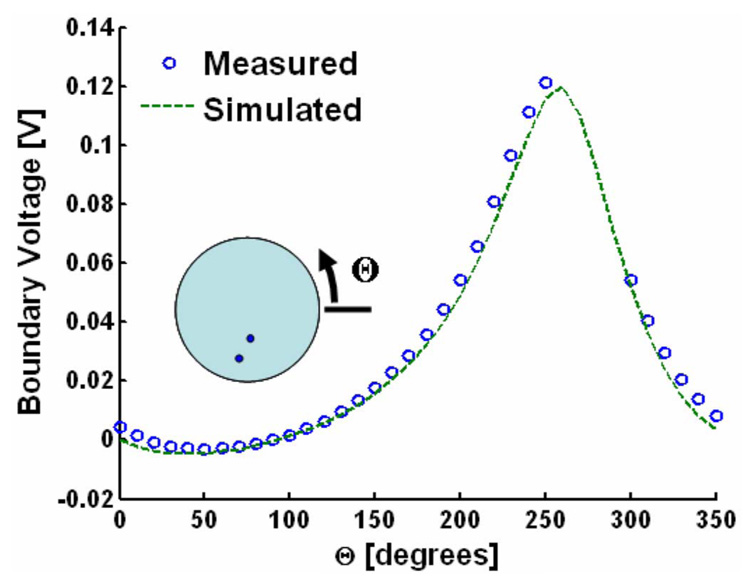
Conventional measurement (open blue circles) and simulation (dashed green line) of the potential distribution at the boundary of the bath generated by the current injected through the stimulation electrodes. Θ is the location at the boundary of the roving tungsten electrode. The inset illustrates the measurement geometry. The current-injecting wires over the bath (illustrated in Fig. 2) prevented measurement in the range Θ = 260°–300°.
Fig. 6.

Sample traces for a single pixel of a single lead. Geometry is illustrated on the right. Trace A) is the pulse echo with the echoes from different features in the picture to the right. Trace B) has two AE traces, one captured when the ultrasound is triggered on the positive peak of the current waveform (+) and the other when the ultrasound is triggered on the negative peak (−). As expected the “+” waveform is 180° out of phase with the “−” waveform. Trace C) is the subtraction of the “−” waveform from the “+” waveform to minimize common-mode interference.
Fig. 7 shows an example of a detected UCSD image for a single angle (Θ =260.). It corresponds to (21). Even for a single lead of two electrodes, the location of the source is highly resolved. There were 16 other similar images—one for each position of the mobile electrode. All 17 images were used to reconstruct the current density as described by (21) and (22). The results of the reconstruction are displayed in Fig. 8 (left). Reconstruction based on experimental results (top row) is consistent with simulated reconstructions (bottom row). The x and y components of the current density, as well as the divergence, are also shown in Fig. 8. Results using a conventional inverse algorithm (i.e., the likelihood as a function of space) are illustrated to the far right [22]. This conventional algorithm, described at the end of Section IV-A, finds the most likely location of a single dipole given the boundary voltage distribution displayed in Fig. 5.
Fig. 7.

A UCSD image for a single lead when the roving electrode is at Θ = 260°, while the reference electrode is still at Θ = 0°, as illustrated with the cartoon above and center. The figure on the right is the actual measurement, while the figure on the left is the theoretical prediction.
Fig. 8.

Left: Reconstruction results for both measured (top row) and simulated (bottom row) data. The left, middle, and right columns correspond to the x-component, y-component, and divergence of the current density, respectively. The “+” signs illustrate extrema positions. Right: Results of a conventional algorithm that finds the most likely position of a single dipole given the low-frequency boundary voltage distribution shown in Fig. 5.
The divergence of the current density is related to the current source density by (23). Reconstructions were quantified by locating the current sources and sinks based on the extrema of the divergence distribution of the simulated and measured data. The estimated and actual positions are summarized in Table I. Simulations agreed well with UCSDI and low-frequency measurements. The reconstructed current field from UCSDI located the current source and sink to within 1 mm of the actual locations. Note that, in this case, the full-width at half-maximum (FWHM) values of UCSDI were dominated by the lateral dimensions of the focal spot of the ultrasound transducer, which was approximately 3 mm, based on its f number (f/#=4) and the center frequency of the AE signal (2 MHz).
TABLE I.
Location estimates of current sources and current sinks. Actual locations refer to independent measurements of current injection electrode positions. The FWHM is twice the mean distance from a given extrema of the divergence to the half-maximum contour. FWHM = Full-Width at Half-Maximum
| Current Source/Sink | Name | X [mm] | Y [mm] | FWHM [mm] |
|---|---|---|---|---|
| Source | Simulated AE | −2.2 | −10.3 | 3.8 |
| Source | Measured AE | −2.3 | −10.3 | 3.8 |
| Source | Actual | −1.7 | −10.8 | |
| Sink | Simulated AE | 0.3 | −5.4 | 3.8 |
| Sink | Measured AE | −0.05 | −3.7 | 4.2 |
| Source | Simulated AE | −2.2 | −10.3 | 3.8 |
| Sink | Actual | 0.7 | −5.3 |
VI. DISCUSSION
We have described UCSDI, a new method to map current densities based on the AE effect with improved spatial resolution. In this initial study under controlled conditions, UCSDI accurately located a 2-D current source to within 1 mm of its actual position, without making prior assumptions about the nature of the source, other than the resistivity distribution. The accuracy was within one sampling interval of the grid-step size (2.2 mm).
The spatial resolution of UCSDI according to the simplified AE signal equation (16) is dominated by the ultrasound beam, due to its sifting property in UCSDI. The thin current-injecting electrodes (diameter = 0.2 mm) can be considered point sources. The average FWHM of 4 mm for both simulated and measured data was consistent with the beamwidth of the transducer (3 mm) and the applied smoothing filter. The lateral resolution can be improved by choosing a transducer with a tighter focus than the f/4 used for this study. The beam spot size of a narrow-band transducer is roughly equal to the product of the wavelength and f/number, where f/number is the ratio of the transducer’s focal length to its diameter. For example, a tightly focused transducer with f/1 at the same frequency would have a focal diameter of approximately 0.75 mm.
The conventional inverse algorithm produced the broad likelihood distribution shown in Fig. 8 (FWHM = 15 mm). The chosen inverse method represents the best-case scenario for conventional algorithms. The dipole source geometry dovetails with the explicit single-dipole assumption, and the algorithm uses multiple measurements (17) with high SNR. In contrast, our method directly resolves the location of the dipole’s source and sink with only the assumption of the resistivity distribution, (in this case, homogenous) which is a necessary assumption of most inverse algorithms. Furthermore, in Fig. 8 a map of the entire 2-D current field is illustrated as an image of the x— and y-components of the field. Direct estimates of the current field would not normally be possible using conventional electrical mapping methods.
Although we demonstrate that UCSDI reconstructs both the magnitude and direction of the current from a synthetic array of 18 electrodes, as few as two electrodes provide detailed information on the actual location of the current dipole (Fig. 7). Conventional dipole localization would require a large number of electrodes to approach similar results, as Fig. 8 demonstrates.
Although these initial results are promising, the approach has limitations. The small AE signal must be conditioned appropriately (filtering, etc), such as that shown in Fig. 6. The effect of the small signal can be seen in the noise ripples in the upper-left quadrant of the detected AE image in Fig. 7. This affected the reconstruction of JX and JY, as illustrated in Fig. 8. However, the SNR of the reconstructed image was still sufficient to accurately estimate the current source and sinks to within 1 mm. Further investigations will be aimed at increasing signal size, while reducing sources of noise.
In this paper, a simple 2-D current system was used, for the sake of clarity, to directly compare UCSDI with other methods for mapping biopotentials. However, it is clear from the AE signal equation (7) that this method can be extended to 3-D and more complicated source geometries. Reconstruction using 3-D will probably be not as straightforward as in the 2-D case for which (7) could be separated into two factors in (16), one that depends only on x and y and the other on z. In a 3-D reconstruction, the dependence of the beam pattern b(x, y, z) on z needs to be taken into account. If the ultrasound transducer and electrode array are fixed in position with respect to each other, a known electrical source can be used to self-calibrate the UCSDI system.
Although this paper focuses on applications of UCSDI to electrocardiography, the technique could also be used for current density analysis in the exposed brain or other neural structures. If this technique were applied to intracardiac electrocardiography, it could potentially generate 3-D current maps of the cardiac activation wave with high spatial resolution. High-frame-rate UCSDI is possible via electronic ultrasound beam steering. Although existing catheters that integrate electrodes with ultrasound are limited to 2-D imaging, technology exists to steer 60° × 60° sectors in 3-D, which might be used to generate 3-D images of current flow coregistered with pulse-echo images illustrating structure [11], [27], [28]. The relative motion of the catheter might not be a significant problem, since the heart is quasi-stationary during the spread of the activation wave. Motion-compensation algorithms could be used to reduce artifacts associated with heart motion [29].
USCDI has unique advantages over other methods because there is no registration error between anatomical images and maps of electrical activity. This is superior to conventional inverse localization methods that use presurgical computed tomography (CT) or MRI images for anatomical mapping fused with an electroanatomical map for catheter guidance. MRI and CT provide presurgical, static images of the heart and typically provide no functional information. Registration error between the CT/MRI images and the electroanatomical map has been reported to be in the range of 2–10 mm [8], [10], [30], [31]. Preliminary studies have shown that a combined electrode and ultrasound catheter can be used for anatomical mapping and guidance [11], [28]. If such a device is made compatible for UCSDI, pulse-echo ultrasound images showing myocardial anatomy and kinematics can be simultaneously integrated with electrical mapping. Such automatic real-time coregistration is currently not found in typical cardiac imaging and would dramatically facilitate guidance during corrective heart surgery.
VII. CONCLUSION
In short, UCSDI has several potential advantages over standard endocardial mapping. This study demonstrates that UCSDI accurately locates sources and sinks to within 1 mm and provides spatial resolution superior to conventional methods. Results were validated using both simulations and direct low-frequency measurements. In addition, UCSDI potentially facilitates conventional electrical mapping procedures with as few as three independent voltage recordings for 3-D localization of current sources. High-frame-rate UCSDI may be possible with electronic beam steering, which would dramatically reduce the time required to map cardiac currents—from hours to seconds. Finally, because of the physics involved, UCSDI is automatically coregistered with B-mode ultrasound., suggesting that an intracardiac catheter would provide real-time mapping of the electrical activity of the heart superimposed on anatomical ultrasound images. Such a device would undoubtedly facilitate electrical mapping of current sources and electrical potentials during interventional surgery.
Acknowledgments
This work was supported in part by the National Institutes of Health under Grant HL67647, Grant EB003451, and Grant HL082640, in part by the Department of Biomedical Engineering at the University of Michigan, and in part by the Fulbright Fellowship Program, U.S. Department of State.
Biographies
Ragnar Olafsson (S’00) received the B.S. degree in electrical engineering in 2002 from the University of Iceland, Reykjavik, Iceland, and the M.S. degree in biomedical engineering in 2004 from the University of Michigan, Ann Arbor. He is currently working toward the Ph.D. degree at the University of Michigan, under Dr. Matthew O’Donnell in the Biomedical Ultrasonics Laboratory.
His current research interests are electrical cardiac imaging using ultrasound current source density imaging and photoacoustics.
Mr. Olafsson was the recipient of a Fulbright Scholarship in 2002.

Russell Witte received the Bachelor’s degree (with honors) in physics from the University of Arizona, Tucson, in 1993, and the Ph.D. degree in bioengineering in 2002.
Following travel abroad in Europe and Brazil, he began graduate school at Arizona State University in bioengineering. His doctoral thesis exploited chronic microelectrode arrays to describe sensory coding and cortical plasticity in the mammalian brain. He then moved to University of Michigan, Ann Arbor, to develop new ultrasound contrast mechanisms for imaging especially brain, nerve, and muscle tissue. While at the Biomedical Ultrasonics Laboratory, he helped devise several novel imaging techniques involving ultrasound. Currently, he is an Assistant Professor of Radiology and Director of the Experimental Ultrasound and Neural Imaging Laboratory at the University of Arizona, where he is engaged in research on new methods using a combination of light, ultrasound, and radiofrequency that potentially impact a variety of medical disorders from epilepsy to cancer.

Sheng-Wen Huang (M’05) was born in Changhua, Taiwan, R.O.C., in 1971. He received the B.S. and Ph.D. degrees in electrical engineering from National Taiwan University, Taipei, Taiwan, in 1993 and 2004, respectively.
He was a Postdoctoral Researcher at National Taiwan University from 2004 to 2005, and is currently a Postdoctoral Researcher with the Department of Biomedical Engineering at the University of Michigan, Ann Arbor. His current research interests include optoacoustic transduction and imaging, ultrasound elasticity imaging, and thermal strain imaging.

Matthew O’Donnell (M’79–SM’84–F’93) reveived the B.S. and Ph.D. degrees in physics from the University of Notre Dame, Notre Dame, IN, in 1972 and 1976, respectively.
Following his graduate work, he moved to Washington University, St. Louis, MO, as a Postdoctoral Fellow in the Department of Physics, where he was engaged in research on applications of ultrasonics to medicine and nondestructive testing. He subsequently held a joint appointment as a Senior Research Associate in the Department of Physics and a Research Instructor of Medicine in the Department of Medicine, Washington University. In 1980 he moved to General Electric Corporate Research and Development Center, Schenectady, NY, where he was engaged in research on medical electronics, including MRI and ultrasound imaging systems. During the 1984–1985 academic year, he was a Visiting Fellow in the Department of Electrical Engineering, Yale University, New Haven, CT, where he was engaged in research on automated image analysis systems. In 1990, he became a Professor of Electrical Engineering and Computer Science at the University of Michigan, Ann Arbor. Starting in 1997, he held a joint appointment as Professor of Biomedical Engineering. In 1998, he was named the Jerry W. and Carol L. Levin Professor of Engineering. During 1999–2006, he also served as Chair of the Department of Biomedical Engineering. In 2006, he moved to the University of Washington, Seattle, where he is currently the Frank and Julie Jungers Dean of Engineering and also a Professor of Bioengineering. His most recent research has explored new imaging modalities in biomedicine, including elasticity imaging, in vivo microscopy, optoacoustic arrays, optoacoustic contrast agents for molecular imaging and therapy, thermal strain imaging, and catheter-based devices.

Contributor Information
Ragnar Olafsson, Department of Biomedical Engineering, University of Michigan, Ann Arbor, MI 48109 USA (e-mail: rolafsso@umich.edu)..
Russell S. Witte, University of Arizona, Tucson, AZ 85724 USA (e-mail: rwitte@radiology.arizona.edu)..
Sheng-Wen Huang, Department of Biomedical Engineering, University of Michigan, Ann Arbor, MI 48109 USA (e-mail: shengwen@umich.edu)..
Matthew O’Donnell, Department of Bioengineering, University of Washington, Seattle, WA 98195 USA (e-mail: donnel@engr.washington.edu)..
REFERENCES
- 1.Klemm HU, Steven D, Johansen C, Ventura R, Rostock T, Lutomsky B, Risius T, Meinertz T, Willems S. Catheter motion during atrial ablation due to the beating heart and respiration: Impact on accuracy and spatial referencing in three-dimensional mapping. Heart Rhythm. 2007;vol. 4:587–582. doi: 10.1016/j.hrthm.2007.01.016. [DOI] [PubMed] [Google Scholar]
- 2.Goldberger JJ. Atrial fibrillation ablation: Location, location, location. J. Cardiovasc. Electrophysiol. 2006 Dec.vol. 17:1271–1273. doi: 10.1111/j.1540-8167.2006.00669.x. [DOI] [PubMed] [Google Scholar]
- 3.Malkin R, Kramer N, Schnitz B, Gopalakrishnana M, Curry A. Advances in electrical andmechanical cardiac mapping. Physiol. Meas. 2005;vol. 26:R1–R14. doi: 10.1088/0967-3334/26/1/r01. [DOI] [PubMed] [Google Scholar]
- 4.Rao L, Sun H, Khoury D. Global comparisons between contact and noncontact mapping techniques in the right atrium: Role of cavitary probe size. Ann. Biomed. Eng. 2001;vol. 29:493–500. doi: 10.1114/1.1376389. [DOI] [PubMed] [Google Scholar]
- 5.Greensite F. Heart surface electrocardiographic inverse solutions. In: He B, editor. Modeling and Imaging of Bioelectric Activity—Principles and Application. New York: Kluwer/Plenum; 2004. pp. 119–160. [Google Scholar]
- 6.Gornick C, Adler S, Pederson B, Hauck J, Budd J, Schweitzer J. Validation of a new noncontact catheter system for electroanatomic mapping of left ventricular endocardium. Circulation. 1999;vol. 99(no 6):829–835. doi: 10.1161/01.cir.99.6.829. [DOI] [PubMed] [Google Scholar]
- 7.Daccarett M, Segerson NM, Gunther J, Nolker G, Gutleben K, Brachmann J, Marrouche NF. Blinded correlation study of three-dimensional electro-anatomical image integration and phased array intracardiac echocardiography for left atrial mapping. Europace. 2007 Oct;vol. 9:923–926. doi: 10.1093/europace/eum192. [DOI] [PubMed] [Google Scholar]
- 8.Heist EK, Chevalier J, Holmvang G, Singh JP, Ellinor PT, Milan DJ, D’Avila A, Mela T, Ruskin JN, Mansour M. Factors affecting error in integration of electroanatomic mapping with CT and MR imaging during catheter ablation of atrial fibrillation. J. Interv. Card. Electrophysiol. 2006;vol. 17:21–27. doi: 10.1007/s10840-006-9060-2. [DOI] [PubMed] [Google Scholar]
- 9.Berger T, Fischer G, Pfeifer B, Modre R, Hanser F, Trieb T, Roithinger FX, Stuehlinger M, Pachinger O, Tilg B, Hintringer F. Single-beat noninvasive imaging of cardiac electrophysiology of ventricular pre-excitation. J. Amer. Coll. Cardiol. 2006;vol. 48(no 10):2045–2052. doi: 10.1016/j.jacc.2006.08.019. [DOI] [PubMed] [Google Scholar]
- 10.Fahmy TS, Mlcochova H, Wazni OM, Patel D, Cihak R, Kanj M, Beheiry S, Burkhardt JD, Dresing T, Hao S, Tchou P, Kautzner J, Schweikert RA, Arruda M, Saliba W, Natale A. Intracardiac echo-guided image integration: Optimizing strategies for registration. J. Cardiovasc. Electrophysiol. 2007;vol. 18:181–186. doi: 10.1111/j.1540-8167.2007.00727.x. [DOI] [PubMed] [Google Scholar]
- 11.Rao L, Ding R, Khoury D. Novel noncontact catheter system for endocardial electrical and anatomical imaging. Ann. Biomed. Eng. 2004;vol. 32(no 4):573–584. doi: 10.1023/b:abme.0000019177.16890.61. [DOI] [PubMed] [Google Scholar]
- 12.Mickelsen S, Dudley B, Treat E, Barela J, Omdahl J, Kusumoto F. Survey of physician experience, trends and outcomes with atrial fibrillation ablation. J. Interv. Card. Electrophysiol. 2005 Apr.vol. 12:213–220. doi: 10.1007/s10840-005-0621-6. [DOI] [PubMed] [Google Scholar]
- 13.Sood S, Chugani HT. Functional neuroimaging in the preoperative evaluation of children with drug-resistant epilepsy. Childs Nerv. Syst. 2006;vol. 22:810–820. doi: 10.1007/s00381-006-0137-0. [DOI] [PubMed] [Google Scholar]
- 14.Olafsson R, Witte RS, O’Donnell M. Measurement of a 2D electric dipole field using the acousto-electric effect. Proc. SPIE Med. Imag. Ultrason. Imag. Signal Process; 2007. p. 65130S. [Google Scholar]
- 15.Witte RS, Olafsson R, Huang S-W, O’Donnell M. Imaging current flow in lobster nerve cord using the acousto-electric effect. Appl. Phy. Lett. 2007;vol. 90(no 16):163902. [Google Scholar]
- 16.Jossinet J, Lavandier B, Cathignol D. Impedance modulation by pulsed ultrasound. Ann. NY Acad. Sci. 1999;vol. 873:396–407. [Google Scholar]
- 17.Jossinet J, Lavandier B, Cathignol D. The phenomenology of acousto-electric interaction signal in aqueous solutions of electrolytes. Ultrasonics. 1998;vol. 36:607–613. doi: 10.1016/s0041-624x(00)00029-9. [DOI] [PubMed] [Google Scholar]
- 18.Lavandier B, Jossinet J, Cathignol D. Experimental measurement of the acousto-electric interaction signal in saline solution. Ultrasonics. 2000;vol. 38:929–936. doi: 10.1016/s0041-624x(00)00029-9. [DOI] [PubMed] [Google Scholar]
- 19.Olafsson R, Witte RS, Kim K, Ashkenazi S, O’Donnell M. Electric current mapping using the acoustoelectric effect. Proc. SPIE Med. Imag. 2006: Ultrason. Imag. Signal Process. vol. 6147:614701. [Google Scholar]
- 20.Witte RS, Olafsson R, O’Donnell M. Acousto-electric detection of current flowin a neural recording chamber. 2006 IEEE Int. Ultrason. Symp.; pp. 5–8. [Google Scholar]
- 21.Zhang H, Wang L. Acousto-electric tomography. Proc. SPIE Photons Plus Ultrasound: Imag. Sens.; 2004. pp. 145–149. [Google Scholar]
- 22.Finke S, Gulrajani RM. Conventional and reciprocal approaches to the inverse dipole localization problem of electroencephalograpy. IEEE Trans. Biomed. Eng. 2003 Jun;vol. 50(no 6):657–666. doi: 10.1109/TBME.2003.812198. [DOI] [PubMed] [Google Scholar]
- 23.Malmivuo J, Plonsey R. Bioelectromagnetism: Principles and Applications of Bioelectric and Biomagnetic Fields. NewYork: Oxford Univ. Press; 1995. [Google Scholar]
- 24.He B, Wu D. Imaging and visualization of 3-D cardiac electric activity. IEEE Trans. Inf. Technol. Biomed. 2001 Sep;vol. 5(no 3):276–282. doi: 10.1109/4233.945288. [DOI] [PubMed] [Google Scholar]
- 25.Angelsen B. Proc. Ultrasound Imag.: Waves Signals Signal Process. vol. I. Norway: Emantec; 2000. Chapter 5: Radiation field from a single element transducers; pp. 5.1–5.97. [Google Scholar]
- 26.Rao NN. Fundamentals of engineering electromagnetics revisited. In: Bansal R, editor. Fundamentals of Engineering Electromagnetics. Boca Raton, FL: CRC: Taylor & Francis; 2006. pp. 1–53. [Google Scholar]
- 27.Lee W, Idriss SF, Wolf PD, Smith SW. A miniaturized catheter 2-D array for real-time, 3-D intracardiac echocardiography. IEEE Trans. Ultrason. Ferroelectr., Freq. Control. 2004 Oct.vol. 51(no 10):1334–1346. doi: 10.1109/tuffc.2004.1350962. [DOI] [PubMed] [Google Scholar]
- 28.Stephens DN, Cannata J, Liu R, Shung KK, Oralkan O, Nikoozadeh A, Khuri-Yakub P, Nguyen H, Chia R, Dentinger A, Wildes D, Thomenius KE, Mahajan A, Shivkumar K, Kim K, O’Donnell M, Sahn DJ. Forward looking intracardiac imaging catheters for electrophysiology. Proc. 2006 IEEE Ultrason. Symp. 06CH37777C; pp. 702–705. [Google Scholar]
- 29.Shi Y, de Ana FJ, Chetcuti SJ, O’Donnell M. Motion artifact reduction for IVUS-based thermal strain imaging. IEEE Trans. Ultrason. Ferroelectr., Freq. Control. 2005 Aug.vol. 52(no 8):1312–1319. doi: 10.1109/tuffc.2005.1509789. [DOI] [PubMed] [Google Scholar]
- 30.Reddy VY, Malchano ZJ, Holmvang G, Schmidt EJ, D’Avila A, Houghtaling C, Chan RC, Ruskin JN. Integration of cardiac magnetic resonance imaging with three-dimensional electroanatomicmapping to guide left ventricular catheter manipulation. J. Am. Coll. Cardiol. 2004;vol. 44(no 11):2202–2213. doi: 10.1016/j.jacc.2004.08.063. [DOI] [PubMed] [Google Scholar]
- 31.Kistler PM, Rajappan K, Jahngir M, Early MJ, Harris S, Abrams D, Gupta D, Liew R, Ellis S, Sporton SC, Schilling RJ. The impact of CT image integration into an electroanatomic mapping system on clinical outcomes of catheter ablation of atrial fibrilliation. J. Cardiovasc. Electrophysiol. 2006 Oct.vol. 17:1093–1101. doi: 10.1111/j.1540-8167.2006.00594.x. [DOI] [PubMed] [Google Scholar]