Higher criticism thresholding: Optimal feature selection when useful features are rare and weak

Abstract

In important application fields today—genomics and proteomics are examples—selecting a small subset of useful features is crucial for success of Linear Classification Analysis. We study feature selection by thresholding of feature Z-scores and introduce a principle of threshold selection, based on the notion of higher criticism (HC). For i = 1, 2, …, p, let π_i denote the two-sided P-value associated with the ith feature Z-score and π_(i) denote the ith order statistic of the collection of P-values. The HC threshold is the absolute Z-score corresponding to the P-value maximizing the HC objective (i/p − π_(i))/$\sqrt{i/p(1-i/p)}$. We consider a rare/weak (RW) feature model, where the fraction of useful features is small and the useful features are each too weak to be of much use on their own. HC thresholding (HCT) has interesting behavior in this setting, with an intimate link between maximizing the HC objective and minimizing the error rate of the designed classifier, and very different behavior from popular threshold selection procedures such as false discovery rate thresholding (FDRT). In the most challenging RW settings, HCT uses an unconventionally low threshold; this keeps the missed-feature detection rate under better control than FDRT and yields a classifier with improved misclassification performance. Replacing cross-validated threshold selection in the popular Shrunken Centroid classifier with the computationally less expensive and simpler HCT reduces the variance of the selected threshold and the error rate of the constructed classifier. Results on standard real datasets and in asymptotic theory confirm the advantages of HCT.

The modern era of high-throughput data collection creates data in abundance; however, this data glut poses new challenges. Consider a simple model of linear classifier training. We have a set of labeled training samples (Y_i, X_i), i = 1, …, n, where each label Y_i is ±1 and each feature vector X_i ∈ R^p. For simplicity, we assume the training set contains equal numbers of 1's and −1's and that the feature vectors X_i ∈ R^p obey X_i ∼ N(Y_iμ, Σ), i = 1, …, n, for an unknown mean contrast vector μ ∈ R^p; here, Σ denotes the feature covariance matrix and n is the training set size. In this simple setting, one ordinarily uses linear classifiers, taking the general form L(X) = Σ_j^p = 1 w(j)X(j), for a sequence of “feature weights” w = (w(j): j = 1, …, p).

Classical theory going back to R. A. Fisher (1) shows that the optimal classifier has feature weights w ∝ Σ⁻¹ μ; at first glance, linear classifier design seems straightforward and settled. However, in many of today's most active application areas, it is a major challenge to construct linear classifiers that work well.

In many ambitious modern applications—genomics and proteomics come to mind—measurements are automatically made on thousands of standard features, but in a given project, the number of observations, n, might be in the dozens or hundreds. In such settings, p ≫ n, which makes it difficult or impossible to estimate the feature covariance straightforwardly. In such settings one often ignores feature covariances. Working in standardized feature space where individual features have mean zero and variance one, a by-now standard choice uses weights w(j) ∝ Cov(Y, X(j)) ≡ μ(j) (2, 3). Even when this reduction makes sense, further challenges remain.

When Useful Features Are Rare and Weak

In some important applications, standard measurements generate many features automatically, few of which are likely to be useful in any specific project, but researchers do not know in advance which ones will be useful in a given project. Moreover, reported misclassification rates are relatively high. Hence, the dimension p of the feature vector is very large, and although there may be numerous useful features, they are relatively rare and individually quite weak.

Consider the following rare/weak feature model (RW feature model). We suppose the contrast vector μ to be nonzero in only k out of p elements, where ε = k/p is small, that is, close to zero. As an example, we might have p = 10,000, k = 100, and so ε = k/p = 0.01. In addition, we suppose that the nonzero elements of μ have common amplitude μ₀. Because the elements X(j) of the feature vector where μ(j) = 0 are entirely uninformative about the value of Y(j), only the k features where μ(j) = μ₀ are useful. The problem is how to identify and benefit from those rare, weak features. Setting $\tau =\sqrt{n}{\mu }_0$, we speak of the parameters ε and τ as the sparsity and strength parameters and denote by RW(ε,τ) this setting. [Related “sparsity” models are common in estimation settings (4, 5). The RW model includes an additional feature strength parameter τ not present in those estimation models. More closely related to the RW model is work in multiple testing by Ingster and the authors (6–8), although the classification setting gives it a different meaning.]

Naïve application of the formula w ∝ Cov(Y, X) in the RW setting often leads to very poor results; the vector of empirical covariances ($\widehat{Co}{v}_{n,p}$(Y, X(j)): j = 1, …, p) is very high-dimensional and contains mostly “noise” coordinates; the resulting naive classification weights ŵ_naive(j) ∝ $\widehat{Co}{v}_{n,p}$(Y, X(j)) often produce correspondingly noisy decisions. The data glut seriously damages the applicability of such “textbook” approaches.

Feature Selection by Thresholding

Feature selection, that is, working only with an empirically selected subset of features, is a standard response to data glut. Here, and below, we suppose that feature correlations can be ignored and that features are standardized to variance one. We consider subset selectors based on the vector of feature Z-scores with components Z(j) = n^−1/2 Σ_iY_iX_i(j), j = 1, …, p. These are the Z-scores of two-sided tests of H_0,j: Cov(Y, X(j)) = 0. Under our assumptions Z ∼ N(θ, I_p), where θ = $\theta =\sqrt{n}\mu$ and μ is the feature contrast vector. Features with nonzero μ(j) typically have significantly nonzero Z(j) and, conversely, other features will have Z(j) consistent with the null hypothesis μ(j) = 0. In such a setting, selecting features with Z-scores above a threshold makes sense. We identify three useful threshold functions: η_t*(z), ★ ∈ {clip, hard, soft}. These are: clipping, η_t^clip(z) = sgn(z), which ignores the size of the Z-score, provided it is large; hard thresholding, η_t^hard(z) = z·1_{{|z| > t}}, which uses the size of the Z-score, provided it is large; and soft thresholding, η_t^soft(z) = sgn(z) (|z| − t)₊, which uses a shrunken Z-score, provided it is large.

Definition 1:

Let ★ ∈ {soft, hard, clip}. The threshold feature selection classifier makes its decision based on L_t^★ <> 0, where L̂_t^★(X) = Σ_j^p = 1 ŵ_t^★(j) X(j), and ŵ_t^★(j) = η_t^★ (Z(j)), j = 1, …, p.

In words, the classifier sums across features with large training-set Z-scores, using a simple function of the Z-score to weight the corresponding feature appropriately.

Well known methods for linear classification follow this approach: The Shrunken Centroids method (9) reduces, in our two-class setting, to a variant of soft thresholding; the schemes discussed in refs. 10 and 11 are variants of hard thresholding.

Thresholding has been popular in estimation for more than a decade (4); it is known to be successful in “sparse” settings where the estimand has many coordinates, of which only a relatively few coordinates are significantly nonzero. Although classification is not the same as estimation, an appropriate theory for thresholding can be constructed (unpublished work) showing that threshold feature classifiers with ideally chosen thresholds work well and even optimally control the misclassification rate.

One crucial question remains: how to choose the threshold based on the data? Related proposals for threshold choice include cross-validation (9), control of the false discovery rate (12–14), and control of the local false discovery rate (15).

Higher Criticism

We propose a method of threshold choice based on recent work in the field of multiple comparisons.

HC Testing.

Suppose we have a collection of N P-values π_i, which under the global null hypothesis are uniformly distributed: π_i ∼_iid U[0,1]. We perform the increasing rearrangement into order statistics: π₍₁₎ ≤ π₍₂₎ ≤ … ≤ π_(N); and we note that, under the null hypothesis, these order statistics have the usual properties of uniform order statistics, including the asymptotic normality π_(i) ∼_approx Normal(i/N, i/N(1 − i/N)). The ordered P-values may be compared with such properties, leading to the following notion.

Definition 2 (HC testing) (7):

The higher criticism (HC) objective is

Fix α₀ ∈ (0, 1) (e.g., α₀ = 1/10). The HC test statistic is HC* = max_{1 ≤ i ≤ α0^N} HC(i; π_(i)).

In practice, HC* is typically insensitive to the selection of α, especially in rare/weak situations. The HC-objective function is the “Z-score of the P-value,” that is, a standardized quantity with asymptotic distribution N(0, 1) under the null hypothesis. In words, we look for the largest standardized discrepancy between the expected behavior of the π_i under uniformity and the observed behavior. When this is large, the whole collection of P-values is not consistent with the global null hypothesis. The phrase “higher criticism” reflects the shift in emphasis from single test results to the whole collection of tests (7). The HC test statistic was developed to detect the presence of a small fraction of non-null hypotheses among many truly null hypotheses (7). Note: there are several variants of HC statistic; we discuss only one variant in this brief note; the main results of ref. 7 still apply to this variant. For full discussion, see ref. 7 and unpublished work by the authors.

HC Thresholding.

Return to the classification setting in previous sections. We have a vector of feature Z-scores (Z(j), j = 1, …, p). We apply HC notions by translating the Z-scores into two-sided P-values, and maximizing the HC objective over index i in the appropriate range. Mixing standard HC notations with standard multivariate data notation requires a bit of care. Please recall that p always refers to the number of measured classifier features, whereas terms such as “P-value” and “π_(i)” refer to unrelated concepts in the HC setting. In an attempt to avoid notational confusion, let N ≡ p and sometimes use N in place of p. Define the feature P-values π_i = Prob{|N(0, 1)| > |Z(i)|}, i = 1, …, N; and define the increasing rearrangement π_(i), the HC objective function HC(i; π_(i)), and the increasing rearrangement |Z|_(i) correspondingly. Here, is our proposal.

Definition 3 (HC thresholding):

Apply the HC test to the feature P-values. Let the maximum HC objective be achieved at index î. The higher criticism threshold (HCT) is the value t̂^HC = |Z|_(î). The HC threshold feature selector selects features with Z-scores exceeding t̂^HC in magnitude.

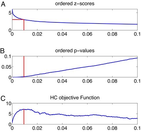
Fig. 1 illustrates the procedure. Fig. 1A shows a sample of Z-scores, B shows a PP plot of the corresponding ordered P-values versus i/N, and C shows a standardized PP plot. The standardized PP plot has its largest deviation from zero at î, and this generates the threshold value.

Fig. 1.

Illustration of HC thresholding. (A) The ordered |Z| scores. (B) The corresponding ordered P-values in a PP plot. (C) The HC objective function in Eq. 1; this is largest at î ≈ 0.01 N (x axes are i/N). Vertical lines indicate π_(î) in B and |Z|_(î) in A.

Performance of HCT in RW Feature Model

In the RW(ε,τ) model, the feature Z-scores vector Z ∼ N(θ, I_p), where θ is a sparse vector with fraction ε of entries all equal to τ and all other entries equal to 0.

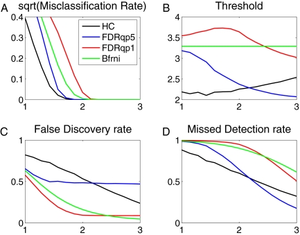
Fig. 2 exhibits results from a collection of problems all with p = 1,000 features, of which only 50 are truly useful, that is, have θ nonzero in that coordinate, so that in each case the fraction of useful features is ε = 50/1,000 = 0.05. In this collection, the amplitude τ of nonzeros varies from 1 to 3. Here, the useful features are indeed weak: they have expected Z-scores typically lower than some Z-scores of useless coordinates.

Fig. 2.

Monte Carlo performance of thresholding rules in the RW model. (A–D) P = 1,000, ε = 0.05, and x axes display τ. (A) MCR^1/2. (B) Average threshold. (C) Average FDR. (D) Average MDR. Threshold procedures used: HC (black), Bonferroni (green), FDR (q = .5) (blue), FDRT (q = .1) (red). Averages from 1,000 Monte Carlo realizations.

We compare HC thresholding with three other thresholding rules: (i) FDRT(.5), thresholding with false feature discovery rate (FDR) control parameter q = 0.5; (ii) FDRT(.1), thresholding with false feature discovery rate control parameter q = 0.1; and (iii) Bonferroni, setting the threshold so that the expected number of false features is 1. These three rules illustrate what we believe to be today's orthodox opinion, which strives to ensure that most features in the classification rule are truly useful, and to strictly control the number of useless features present in the trained classifier. Local false discovery rate control shares the same philosophy. We generated 1,000 Monte Carlo realizations at each choice of parameters. We present results in terms of the dimensionless parameter τ, which is independent of n; if desired, the reader may choose to translate these results into the form μ₀ = τ/$\sqrt{n}$ for a conventional choice of n, such as n = 40. Fig. 2 presents the empirical average performance. As compared with traditional approaches, HCT has, in the case of weak signals, a lower threshold, a higher false-feature discovery rate, and lower missed-feature detection rate (MDR); the misclassification rate (MCR) is also improved. In these displays, as the signal strength τ increases, HCT increases, but FDRT decreases (for analysis of this phenomenon, see unpublished work).

HCT Functional and Ideal Thresholding

We now develop connections between HCT and other important notions.

HCT Functional.

The HCT functional is, informally, the “threshold that HCT is trying to estimate.” More precisely, note that, in the RW(ε, τ) model, the empirical distribution function F_n,p of feature Z-scores F_n,p(t) = Ave_jI{Z(j) ≤ _t}, approximates, for large p and n arbitrary, the theoretical CDF F_ε,τ(t) = (1 − ε) Φ(t) + εΦ(t − τ), t ∈ R, where Φ(t) = P{N(0, 1) ≤ t} is the standard normal distribution. The HCT functional is the result of the HCT recipe on systematically replacing F_n,p(t) by F_ε,τ(t).

We define the underlying true positive rate, TPR(t); the false positive rate, FPR(t); and the positive rate, PR(t), in the natural way as the expected proportions of, respectively, the useful, the useless, and of all features, having Z-scores above threshold t. The HC objective functional can be rewritten (up to rescaling) as

In the RW(ε,τ) model, we have TPR(t; ε, τ) = Φ(t − τ) + Φ(−t − τ), FPR(t; ε, τ) = 2Φ(−t), and PR(t; ε, τ) = (1 − ε) FPR(t) + ε·TPR(t). Let t₀ = t₀(ε,τ) denote the threshold corresponding to the maximization limit α₀ in Definition 2: PR(t₀; ε,τ) = α₀. The HCT functional solves a simple maximization in t:

Rigorous justification of this formula is supplied in ref. 12, showing that in the RW(ε,τ) model, t̂_n,p^HC converges in probability to T_HC(F_ε, τ) as p goes to infinity with n either fixed or increasing; so indeed, this is what HCT is “trying to estimate.”

Ideal Threshold.

We now study the threshold that (if we only knew it!) would provide optimal classifier performance. Recall that, in our setting, the feature covariance is the identity Σ = I_p; the quantity Sep(w; μ) = w′μ/‖w‖₂ is a fundamental measure of linear classifier performance. The misclassification rate of the trained weights ŵ on independent test data with true contrast vector μ obeys

where again Φ is the standard normal N(0, 1) CDF. Hence, maximizing Sep is a proxy for minimizing misclassification rate (for more details, see unpublished work).

For a fixed threshold t, let Sep(w_clip^t; μ) denote the realized value of Sep on a specific realization. For large p and n arbitrary, this is approximately proportional to

where TPR and PR are the true and positive rates defined earlier, and TSER(t) denotes the expected True Sign Error Rate TSER(t) ≡ P{Z(j) < 0|μ(j) > 0}. We are in the RW model, so (t;ε,τ) can be written in terms of TPR(t; ε, τ), PR(ε, τ), and TSER(t; τ) = Φ(−t −τ). We define the ideal threshold functional

Among all fixed thresholds, it achieves the largest separation for a given underlying instance of the RW(ε, τ) model.

Comparison.

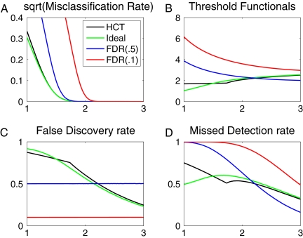
How does the HCT functional compare with the ideal threshold functional, both in value and performance? They seem surprisingly close. Fig. 3 presents the values, FDR, MDR, and MCR for these functionals in cases with ε > 0 fixed and τ varying. The HCT functional quite closely approximates the ideal threshold, both in threshold values and in performance measures. In particular, we note that the behavior of the HCT rule that was so distinctive in the rare/weak features model—high false-feature discovery rate and controlled missed detection rate—are actually behaviors seen in the ideal threshold classifier as well. The systematic discrepancy between the HCT and the ideal threshold at small τ is due to the constraint t > t₀ in Eq. 3.

Fig. 3.

Comparison of HCT functional with ideal functional. In all of the panels, ε = 1/100, and x axes display τ. (A) MCR^1/2. (B) Threshold. (C) FDR. (D) MDR. Threshold procedures used: HC (black), Ideal (green). Curves for FDR thresholding with q = .5 (blue) and q = .1 (red) are also shown. In each measure, green and black curves are close for τ > 2. The discrepancy at small τ is caused by the limitation T_HC > t₀.

ROC Analysis.

The similarity between the HCT functional and the ideal threshold functional derives from the expressions for PR(t; ε, τ) and TPR(t; ε, τ) in the RW model. In the setting where very few features are selected, (1 − PR(t)) ≈ 1, and 2TSER(t) ≪ TPR(t), so we see by comparison of Eqs. 2 and 5 that (t; ε, τ) ≈ $\widetilde{Sep}$(t; ε, τ), as reflected in Fig. 3 (for more discussion and analysis, see unpublished work).

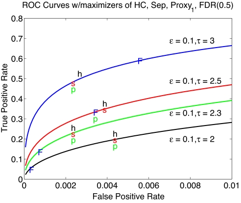
Consider two related expressions: Proxy₁ = ε·TPR(t)/$\sqrt{\text{PR}(t)}$, Proxy₂ = ε·TPR(t)/$\sqrt{\text{FPR}(t)}$. Maximizing either of these proxies over t is equivalent to seeking a certain point on the so called receiver-operating characteristics (ROC) curve (FPR(t),TPR(t) : 0 < t < ∞). Fig. 4 shows a range of ROC curves; the maximizers of (t), of $\widetilde{Sep}$(t), and of Proxy₁(t) are very close in the ROC space. Since the misclassification rate MCR(t) = (1 − ε)(1 − FPR)(t) + ε·(1 − TPR)(t) is a Lipschitz function of the ROC coordinates, all three maximizers must offer similar performance.

Fig. 4.

Receiver operating characteristics curves for threshold detectors, together with operating points of max-HCT (h), max-SEP (s), and max-Proxy₁ (p). Also included are the operating points of FDR (F) thresholding with q = .5. Note that h, s, and p are quite close to each other, but F can be very different.

The maximizer of Proxy₂ has a very elegant characterization, as the point in t where the secant to the ROC curve is double the tangent to the ROC curve, $\frac{TPR\prime }{FPR\prime }=\frac{TPR}{2FPR}$ at t = t_Proxy2. The maximizer of Proxy₁ obeys a slightly more complex relationship $\frac{\text{TPR}\prime }{\text{FPR}\prime }=\text{(2}\frac{\text{FPR}}{\text{TPR}}$ (1 − ε/2)(1 − ε) + ε)⁻¹ at t = t_Proxy1. For small enough ε, this nearly follows the same rule: secant ≈2× tangent.

For comparative purposes, FDR thresholding finds a point on the ROC curve with prescribed secant: $\frac{\text{TPR}}{\text{FPR}}=\frac{\text{1-ε}}{\text{ε}}$ ε(q⁻¹ − 1) at t = − εε(q⁻¹ − 1) at t = t_FDR,q. Further, a local false discovery rate threshold yields a point on the ROC curve with prescribed tangent $\frac{\text{TPR}\prime }{\text{FPR}\prime }=\frac{\text{1-ε}}{\text{ε}}$ (q⁻¹ − 1) at t = t_localFDR,q. Defining the true discovery rate TDR ≡ 1 − FDR, we see that HCT obeys $\frac{\text{FDR}}{\text{TDR}}\approx \frac{\text{1}}{\text{2}}\frac{\text{local}\text{FDR}}{\text{local}\text{TDR}}$, at t = t_Proxy2. HCT and its proxies are thus visibly quite different from prescribing FDR or local FDR, which again underscores the distinction between avoiding false-feature selection and maximizing classifier performance.

Complements

Performance on Standard Datasets.

In recent literature on classification methodology, a collection of six datasets has been used frequently for illustrating empirical classifier performance (16). We have reservations about the use of such data to illustrate HCT, because no one can say whether any specific such dataset is an example of rare/weak feature model. However, such comparisons are sure to be requested, so we report them here.

Of the standard datasets reported in ref. 16, three involve two-class problems of the kind considered here; these are the ALL (10), Colon (17), and Prostate (18) datasets. In ref. 17, 3-fold random training test splits of these datasets were considered, and seven well known classification procedures were implemented: Bagboost (16), LogitBoost (19), SVM (20), Random Forests (21), PAM (9), and the classical methods DLDA and KNN. We applied HCT in a completely out-of-the-box way by using definitions standard in the literature. HCT-hard, which uses feature weights based on hard thresholding of feature Z-scores, gave quite acceptable performance. For comparison, introduce the relative regret measure Regret(A) = [err(A) − min_A′err(A′)]/[max_A′err(A′) − min_A′err(A′)]. This compares the achieved error rate with the best and worst performance seen across algorithms. We report errors rates and regrets side by side in Table 1, where rows 2–7 are from Dettling (16), row 8 is provided by Tibshirani, and row 9 is the result of HCT-hard.

Table 1.

Error rates of standard classifiers on standard examples from Dettling (16)

Method	ALL/reg	Col/reg	Pro/reg	m-reg	R
Bagboo	4.08/0.59	16.10/0.52	7.53/0	0.59	6
Boost	5.67/1	19.14/1	8.71/0.18	1	7.5
RanFor	1.92/0.02	14.86/0.32	9.00/0.22	0.32	2
SVM	1.83/0	15.05/0.35	7.88/0.05	0.35	3
DLDA	2.92/0.28	12.86/0	14.18/1	1	7.5
KNN	3.83/0.52	16.38/0.56	10.59/0.46	0.56	5
PAM	3.55/0.45	13.53/0.11	8.87/0.20	0.45	4
HCT	2.86/0.27	13.77/0.14	9.47/0.29	0.29	1

reg, regret; col, colon; Pro, prostate; m-reg, maximum regret; R, rank based on m-reg.

Additionally, column 5 is the maximum regret across three different datasets, and column 6 is the rank based on the maximum regret. In the random-split test, HCT-hard was the minimax regret procedure, always being within 29% of the best known performance, whereas every other procedure was worse in relative performance in at least some cases.

It is worth remarking that HCT-based feature selection classifiers are radically simpler than all of the other methods being considered in this competition, requiring no tuning or cross-validation to achieve the presented results.

Comparison to Shrunken Centroids.

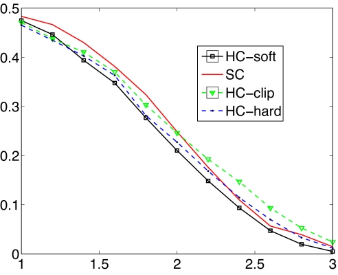
The well known “Shrunken Centroids” (SC) algorithm (9) bears an interesting comparison to the procedures discussed here. In the two-class setting, SC amounts to linear classification with feature weights obtained from soft thresholding of feature Z-scores. Consequently, HCT-soft can be viewed as a modification to SC, choosing thresholds by HCT rather than cross-validation. We made a simulation study contrasting the performance of SC with HCT-hard, HCT-soft, and HCT-clip in the rare/weak features model. We conducted 100 Monte Carlo simulations, where we chose p = 10.000, k = 100 (so ε = k/p = 0.01), n = 40, and τ ∈ [1,3]. Over this range, the best classification error rate ranged from nearly 50%—scarcely better than ignorant guessing—to <3%. Fig. 5 shows the results. Apparently, HCT-soft and SC behave similarly—with HCT-soft consistently better (here SC is implemented with a threshold picked by 10-fold cross-validations). However, HCT-soft and SC are not at all similar in computational cost at the training stage, as HCT-soft requires no cross-validation or tuning. The similarity of the two classifiers is, of course, explainable by using discussions above. Cross-validation is “trying” to estimate the ideal threshold, which the HCT functional also approximates. In Table 2, we tabulated the mean and standard deviation (SD) of HCT and cross-validated threshold selection (CVT). We see that CVT is on average larger than the HCT in this range of parameters. We also see that CVT has a significantly higher variance than the HC threshold; presumably, this is why HCT-soft consistently outperforms SC. In fact, cross-validation is generally inconsistent in the fixed-n, large-p limit, whereas HCT is consistent in the RW model; hence the empirical phenomenon visible in these graphs should apply much more generally.

Fig. 5.

Comparison of error rates by using Shrunken Centroids, threshold choice by cross-validation, and linear classifiers by using HCT-based threshold selection. Simulation assuming the RW model. Black, HCT-soft; red, Shrunken Centroids; green, HCT-clip; blue, HCT-hard. x axis displays τ.

Table 2.

Comparison of HCT and CVT

τ	HCT mean	CVT mean	HCT SD	CVT SD
1.0	2.2863	3.8192	0.3746	1.9750
1.4	2.2599	3.3255	0.3401	1.7764
1.8	2.2925	3.0943	0.3400	1.3788
2.2	2.3660	2.6007	0.2921	0.8727
2.6	2.5149	2.5929	0.2644	0.5183
3.0	2.6090	2.9904	0.2698	0.5971

Alternative Classifier by Using HC.

HC can be used directly for classification (22), without reference to linear discrimination and feature selection (for comparison with the method proposed here, see unpublished work).

Theoretical Optimality.

In a companion article (unpublished work), we developed a large-p, fixed-n asymptotic study and showed rigorously that HCT yields asymptotically optimal error rate classifiers in the RW model.

Reproducible Research.

All original figures and tables presented here are fully reproducible, consistent with the concept of Reproducible Research (23).

References

- 1.Anderson TW. An Introduction to Multivariate Statistical Analysis. 3rd Ed. New York: Wiley; 2003. [Google Scholar]
- 2.Bickel P, Levina E. Some theory of Fisher's linear discriminant function, ‘naive Bayes’, and some alternatives when there are many more variables than observations. Bernoulli. 2004;10:989–1010. [Google Scholar]
- 3.Fan J, Fan Y. High dimensional classification using features annealed independence rules. Ann Statist. 2008 doi: 10.1214/07-AOS504. in press. [DOI] [PMC free article] [PubMed] [Google Scholar]
- 4.Donoho D, Johnstone I. Minimax risk over lp-balls for lq-error. Probab Theory Relat Fields. 1994;2:277–303. [Google Scholar]
- 5.Donoho D, Johnstone I, Hoch JC, Stern AS. Maximum entropy and the nearly black object. J R Stat Soc B. 1992;54:41–81. [Google Scholar]
- 6.Ingster YI. Some problems of hypothesis testing leading to infinitely divisible distribution. Math Methods Stat. 1997;6:47–69. [Google Scholar]
- 7.Donoho D, Jin J. Higher criticism for detecting sparse heterogeneous mixtures. Ann Stat. 2004;32:962–994. [Google Scholar]
- 8.Jin J. Stanford: Department of Statistics, Stanford University; 2003. Detecting and estimating sparse mixtures. Ph.D. thesis. [Google Scholar]
- 9.Tibshirani R, Hastie T, Narasimhan B, Chu G. Diagnosis of multiple cancer types by shrunken centroids of gene expression. Proc Natl Acad Sci USA. 2002;99:6567–6572. doi: 10.1073/pnas.082099299. [DOI] [PMC free article] [PubMed] [Google Scholar]
- 10.Golub T, et al. Molecular classification of cancer: Class discovery and class prediction by gene expression monitoring. Science. 1999;286:531–536. doi: 10.1126/science.286.5439.531. [DOI] [PubMed] [Google Scholar]
- 11.Hedenfalk I, et al. Gene-expression profile in hereditary breast cancer. N Engl J Med. 2001;344:539–548. doi: 10.1056/NEJM200102223440801. [DOI] [PubMed] [Google Scholar]
- 12.Benjamini Y, Hochberg Y. Controlling the false discovery rate: A practical and powerful approach to multiple testing. J R Stat Soc B. 1995;57:289–300. [Google Scholar]
- 13.Abramovich F, Benjamini Y. In: Wavelets and Statistics. Antoniadis A, Oppenheim G, editors. New York: Springer; 1995. pp. 5–14. [Google Scholar]
- 14.Abramovich F, Benjamini Y, Donoho D, Johnstone I. Adapting to unknown sparsity by controlling the false discovery rate. Ann Stat. 2006;34:584–653. [Google Scholar]
- 15.Efron B, Tibshirani R, Storey J, Tusher V. Empirical Bayes analysis of a microarray experiment. J Am Stat Assoc. 2001;99:96–104. [Google Scholar]
- 16.Dettling M. BagBoosting for tumor classification with gene expression data. Bioinformatics. 2004;20:3583–3593. doi: 10.1093/bioinformatics/bth447. [DOI] [PubMed] [Google Scholar]
- 17.Alon U, et al. Broad patterns of gene expression revealed by clustering analysis of tumor and normal colon tissues probed by oligonucleotide arrays. Proc Natl Acad Sci USA. 1999;96:6745–6750. doi: 10.1073/pnas.96.12.6745. [DOI] [PMC free article] [PubMed] [Google Scholar]
- 18.Singh D, et al. Gene expression correlates of clinical prostate cancer behavior. Cancer Cell. 2002;1:203–209. doi: 10.1016/s1535-6108(02)00030-2. [DOI] [PubMed] [Google Scholar]
- 19.Dettling M, Bühlmann P. Boosting for tumor classification with gene expression data. Bioinformatics. 2003;19:1061–1069. doi: 10.1093/bioinformatics/btf867. [DOI] [PubMed] [Google Scholar]
- 20.Burges C. A tutorial on support vector machines for pattern recognition. Knowl Discov Data Min. 1998;2:121–167. [Google Scholar]
- 21.Breiman L. Random forests. Mach Learn. 2001;24:5–32. [Google Scholar]
- 22.Hall P, Pittelkow Y, Ghosh M. Theoretical measures of relative performance of classifiers for high dimensional data with small sample sizes. J R Stat Soc B. 2008;70:158–173. [Google Scholar]
- 23.Donoho D, Maleki A, Ur-Rahman I, Shahram M, Stodden V. Technical report. Stanford: Department of Statistics, Stanford University; 2008. 15 years of reproducible research in computational harmonic analysis. [Google Scholar]