

Abstract
The [FeFe] hydrogenase from the green alga Chlamydomonas reinhardtii can catalyze the reduction of protons to hydrogen gas using electrons supplied from photosystem I and transferred via ferredoxin. To better understand the association of the hydrogenase and the ferredoxin, we have simulated the process over multiple timescales. A Brownian dynamics simulation method gave an initial thorough sampling of the rigid-body translational and rotational phase spaces, and the resulting trajectories were used to compute the occupancy and free-energy landscapes. Several important hydrogenase-ferredoxin encounter complexes were identified from this analysis, which were then individually simulated using atomistic molecular dynamics to provide more details of the hydrogenase and ferredoxin interaction. The ferredoxin appeared to form reasonable complexes with the hydrogenase in multiple orientations, some of which were good candidates for inclusion in a transition state ensemble of configurations for electron transfer.
INTRODUCTION
The photobiological generation of hydrogen gas by the green alga Chlamydomonas reinhardtii provides a promising pathway for renewable hydrogen production (1–7). The H2-production process of C. reinhardtii is sensitive to O2 (8). Although oxygenic photosynthesis and H2 production would thus appear to be incompatible, it has been possible to find conditions under which the O2 production activity of photosystem II (PSII) is decreased enough to induce hydrogenase activity. For instance, when the environmental sulfur supplies are limiting in sealed cultures, the rates of photosynthetic O2 evolution decrease (9) and respiration rapidly consumes the remaining O2, thereby creating an anaerobic environment (9–14). At the same time, the activity in photosystem I (PSI) is preserved and the photochemical energy absorbed by PSI is converted into electrochemical energy in the form of low-potential electrons that are transferred to soluble ferredoxins. Photooxidized PSI may be reduced by the chloroplastic quinone pool, which is in turn kept reduced by residual PSII activity as well as by some of the reducing equivalents originally stored as starch during sulfur-replete conditions (15–17). Thus, by alternating between conditions of sulfur exposure and deprivation, hydrogen gas can be produced in a sustainable way (11).
Optimizing this process to permit simultaneous water oxidation and proton reduction at high PSII and PSI activity would be desirable, and several challenges that would arise in such a system remain to be addressed. Among these is the multiplicity of partners for PSI-reduced ferredoxin under normal growth conditions, which include ferredoxin-NADP+ reductase (FNR) to generate reductant for CO2 fixation, and hydrogenase to generate hydrogen gas (7,18). The Michaelis-Menten constant (KM) of FNR versus hydrogenase for reduced ferredoxin (FNR KM values of 0.4 μM (19) versus hydrogenase KM values of 10–35 μM (20,21)), suggests that the CO2 fixation pathway through FNR might be a preferred electron sink to H2 production. The electron flux through these two competing pathways is in part a function of the thermodynamic and kinetic parameters for the ferredoxin-dependent reduction of each enzyme. Since FNR is one of the central enzymes in the photosynthetic pathway, one long-term possibility to optimize biological hydrogen production is to engineer the hydrogenase-ferredoxin interaction to divert greater electron flux to this pathway. For this reason, and to better understand the mechanism of electron transfer between the [2Fe-2S] ferredoxin and hydrogenase, detailed information on how the hydrogenase interacts with the ferredoxin is required. Compared to the studies on interactions between FNR and ferredoxin (22–27), relatively few studies on the hydrogenase-ferredoxin interaction (18,20,21,28) exist and experimental data are limited. There are two hydrogenases (HydA1 and HydA2) (29) and at least six [2Fe-2S] ferredoxins (PetF1-PetF6) (30) encoded in the C. reinhardtii genome. Although structures for the hydrogenase and hydrogenase-ferredoxin complex from C. reinhardtii are still unknown, it is possible to use computational methods to build models. Chang et al. used homology modeling and rigid-body docking to simulate a hydrogenase (HydA2)-ferredoxin (PetF1) electron-transfer complex (31). Filtered by the intermetallocluster distance and refined by the potential energy calculation, two candidates for a hydrogenase-ferredoxin binding complex were identified, which in keeping with the previous work are referred to here by their original index numbers 16 and 42. Of these, complex 16 was determined to have a lower binding free energy. Therefore, complex 16 was suggested to more likely represent an in vivo interacting configuration between the hydrogenase and ferredoxin during electron transfer (31).
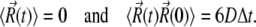
The structures of the hydrogenase-ferredoxin complexes 16 and 42 are shown in Fig. 1. The major difference between these two structures is the orientation of the ferredoxin with respect to the hydrogenase. The two structures are related by an ∼180° rotation of the ferredoxin around the axis from the [4Fe4S]H subcluster of the hydrogenase catalytic center H-cluster to the [2Fe2S]F cluster of the ferredoxin. The binding interface on the hydrogenase has many positively charged residues and the binding interfaces on the ferredoxin are mainly negatively charged, which is consistent with the role of charge-charge interaction in mediating formation of electron-transfer complexes (18). The detailed structures of the ferredoxin [2Fe2S]F cluster and H-cluster are shown in Fig. 2. The redox active [2Fe2S]F cluster of the ferredoxin functions as the electron carrier. During an electron-transfer event, the reduced ferredoxin binds to the hydrogenase and transfers a single electron to the hydrogenase H-cluster. The hydrogenase catalytic center H-cluster consists of a [4Fe4S]H cubane metallocluster and a [2Fe]H metallocluster. These two metalloclusters are covalently bonded together via a conserved cysteine (33). Two successive electron transfer events are required for a single catalytic cycle by the hydrogenase to produce one molecule of hydrogen gas.
FIGURE 1.

Structures of complex 16 (left) and complex 42 (right). Neutral residues of the hydrogenase are in cyan and those of the ferredoxin in lime green. The metalloclusters shown are the hydrogenase H-cluster and the ferredoxin [2Fe2S]F cluster. Positively charged residues on both proteins are shown in red, and negatively charged residues in blue. The pictures in Figs. 1–4 and 11, and in Table 2, were generated by VMD (32).
FIGURE 2.

Detailed structures of the ferredoxin [2Fe2S]F cluster and the [4Fe4S]H and [2Fe]H clusters of the hydrogenase in complex 16.
Brownian dynamics (BD) has been widely used in recent years to study the protein association process (34–40). In most BD simulations, proteins are treated as rigid bodies and are moved by the Brownian forces stochastically (41). The long-range electrostatic force and desolvation effects are considered, whereas short-range interactions such as hydrogen bonding, van der Waals forces, and explicit salt bridges, are neglected. Simplifying the force treatment gives the BD method the ability to simulate molecules over microsecond timescales within reasonable computational time. The BD simulation method has successfully reproduced experimentally measured protein association rates (36,42,43), as well as the transient encounter complexes during the association process (44). A free energy landscape analysis method based on the BD simulation trajectories was developed recently to identify encounter complexes and to detail reaction pathways (45–47). When the two proteins are closer, however, short-range interactions become important. Therefore, more detailed (but slower) molecular dynamics (MD) simulations are required to simulate the dynamics of the encounter complex.
Based on the structures of complexes 16 and 42, we investigated the dynamics of the ferredoxin PetF1 association with the hydrogenase HydA2 using BD and all-atom MD simulations. Free energy landscapes were computed from BD trajectories, and the reaction pathways, as well as the encounter complexes, were identified. The details of the association dynamics in the encounter complexes were further characterized by atomistic MD.
METHODS
Reference structures
Based on the model structures of C. reinhardtii hydrogenase-ferredoxin complexes 16 and 42 (31), we ran BD and MD simulations with the hydrogenase in the oxidized state and the ferredoxin in both reduced and oxidized states. The CHARMM22 atomic charges and atom radii (48) were used for the amino acid residues of the hydrogenase and the ferredoxin in electrostatic potential calculations and MD simulations. The partial atomic charges and radii for the metalloclusters were derived from geometry-optimized model clusters, using a BLYP/6-31+G(d) model chemistry and Natural Population Analysis charges (49) (manuscript in preparation). We note that although this charge derivation procedure differs from the canonical CHARMM method, Meuwly and Karplus have found key dynamical features around the [3Fe4S] cluster of the Azotobacter vinelandii 7Fe ferredoxin insensitive to the particular charge model (50).
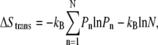
In the reduced state, the ferredoxin [2Fe2S]F cluster and the accompanying four cysteine sulfur ligands (from  and
and  ) have a total partial charge of −3, whereas in the oxidized state the total partial charge is −2. In this research, we assumed that the conformations of the reduced and oxidized ferredoxin were identical except for the peptide bond between residues
  and
and  In the oxidized state,
  -CO points to the [2Fe2S]F cluster, whereas in the reduced state, the
  -CO points away because of larger charge repulsion (Fig. 3) as reported by Morales et al. (51) The pKa values of the charged residues on the reduced and oxidized ferredoxin were calculated using H++ (52,53). We found that the redox state of the [2Fe2S]F cluster had a very weak influence on the pKa values and the protonation states of the charged residues on the ferredoxin remained the same at different [2Fe2S]F redox states at pH 7.0 (Supplementary Material, Table S1, Data S1). For the hydrogenase, we only simulated the hydrogenase with the H-cluster in the oxidized state. The total partial charge on the [2Fe]H cluster is −1, and the [4Fe4S]H cluster, along with the four cysteine sulfur ligands (from
  and
and  ), has a total partial charge of −2.
FIGURE 3.

Conformational switch in the peptide bond between  and
and  for the oxidized (A) and reduced ferredoxin (B). The [2Fe2S]F cluster and the -C(=O)NH- peptide bond between the two residues are in CPK format, and the ferredoxin backbone is in tube format.
Brownian dynamics simulations
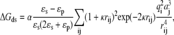
We used the Brownian dynamics simulation program package Simulation of Diffusional Association (SDA) (54) to perform the BD simulations. We simulated a total of four systems: BD16R, the atomic coordinates of the hydrogenase and ferredoxin from the energy-minimized structure of complex 16, with the ferredoxin in the reduced state; BD16O, based on the complex 16 structure with an oxidized ferredoxin; BD42R, based on the complex 42 structure with a reduced ferredoxin; and BD42O, based on the complex 42 structure with an oxidized ferredoxin. During the BD simulation, both hydrogenase and ferredoxin were treated as rigid bodies. The center of mass (COM) of the hydrogenase was fixed in the center of the simulation sphere, and rotational movement was allowed. The ferredoxin moved stochastically around the hydrogenase both translationally and rotationally. The BD simulations started at b = 100 Å of COM-COM distance between the hydrogenase and ferredoxin, and were terminated if the two proteins achieved a COM-COM distance of c > b. To improve the sampling statistics in the region close to the hydrogenase for the free energy landscape analysis, we used a small c = 120 Å. The BD simulations were performed at 50 mM, 150 mM, 300 mM, and 500 mM. At each ionic strength, 50,000 trajectories were generated.
The electrostatic interactions during the simulation were calculated using the following method. First, the electrostatic potential grid around each protein was calculated using the Adaptive Poisson-Boltzmann Solver (APBS) program (55) to solve the full Poisson-Boltzmann equation at the given ionic strength. The grid was centered at each protein and had a dimension of 161 × 161 × 161 with a spacing size of 1 Å, as required by the SDA program. The solvent dielectric constant, ɛs, was 78.5 and the protein interior dielectric constant, ɛp, was set to 4.0. For details of the APBS calculation parameters, please refer to the sample APBS input file (Supplementary Material, Table S2, Data S1). Next, the effective charges on each protein were calculated by the ECM (Effective Changes for Macromolecules in solvent) module (56) in the SDA package. The effective charges are fitted to reproduce the molecular electrostatic potentials calculated by APBS. Finally, the charge desolvation penalty grid was calculated using the mk_ds_grd program in the SDA package (54). The desolvation energy for ferredoxin due to the presence of hydrogenase was computed according to
 |
(1) |
where α is the scaling factor and we used a value of 1.67 from Gabdoulline and Wade (42); κ is the Debye-Hückel screening parameter, which depends on the given ionic strength; i and j denote atom i of the ferredoxin and atom j of the hydrogenase, respectively; q is the effective charge; a is the atomic radius; and rij is the distance between the two atoms. The desolvation energy for the hydrogenase due to the presence of the ferredoxin was computed in a similar way. During the BD simulation, the electrostatic interaction on the hydrogenase (or ferredoxin) was then computed using the effective charges on the hydrogenase (or ferredoxin) and the electrostatic potential grid of the ferredoxin (or hydrogenase). The charge desolvation penalty was calculated similarly using the effective charges and desolvation penalty grids. In this way, the energies could be evaluated much more quickly.
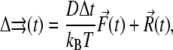
The BD trajectory was propagated by solving the diffusion equations. The translational diffusion equation is
 |
(2) |
where D is the relative translational diffusion constant, Δt is the time step,  is the instantaneous systematic potential force, kB and T are the Boltzmann constant and temperature, respectively (T = 298 K in this work), and
  is the random displacement due to the collisions between the protein and the solvent molecules. The values of
  satisfy the boundary conditions
 |
(3) |
The rotational diffusion equations for both hydrogenase and ferredoxin were solved in a similar way. The translational and rotational diffusion constants for the hydrogenase and ferredoxin were calculated by the program HYDROPRO (57) and the results are presented in Table 1. The calculated diffusion constants are similar to the diffusion constants of similarly sized proteins (42).
TABLE 1.
Brownian dynamics simulation parameters
| Complex 16 | Complex 42 | |
|---|---|---|
| Relative translational diffusion constant (Å2/ps) | 2.160 × 10⁻² | 2.165 × 10⁻² |
| Rotational diffusion constant of ferredoxin (rad2/ps) | 3.016 × 10⁻⁵ | 2.937 × 10⁻⁵ |
| Rotational diffusion constant of hydrogenase (rad2/ps) | 5.918 × 10⁻⁶ | 6.289 × 10⁻⁶ |
The BD simulation time step Δt was chosen as 1.0 ps when the COM-COM distance of the two proteins was within 80 Å. Since the relative translational diffusion constant, D, of the ferredoxin versus the hydrogenase is ∼0.02 Å2/ps, the average movement per step is only 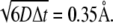 At larger separation distances, Δt was increased linearly with a slope of 0.5 ps/Å.
Free energy landscape calculations
The free energy landscape calculation process is similar to that used by Spaar et al. (46,47). The trajectories of the BD simulations, along with the potential energy information, were stored and used for the free energy landscape calculations. To obtain the free energy, however, the entropy must be calculated. The entropy depends on the spatial and orientational distributions of the ferredoxin, which can be computed from the occupancy landscapes. For that reason, the free energy landscape was computed in three steps. First, the BD simulation trajectories were used to create the spatial and orientational occupancy landscapes of the ferredoxin. Second, from the occupancy landscapes, local entropy-loss landscapes were computed. Finally, based on the entropy-loss landscapes and the potential energy information in the trajectories, the free energy landscape was generated.
The computation of the spatial occupancy landscape
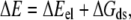
To analyze the BD trajectories of BD16R and BD16O, a reference coordinate system was constructed based on the bound structure of complex 16 (Fig. 4 A). The origin of the reference coordinate system was at the COM of the hydrogenase in the complex. The z axis direction points to the COM of the ferredoxin. Without loss of generality, the y axis direction was assigned as the normal vector of the plane that included the two COMs and the N-terminal nitrogen (N1) of the hydrogenase. For analyzing BD42R and BD42O trajectories, a similar reference coordinate system was constructed based on the bound structure of complex 42.
FIGURE 4.

(A) Definition of the reference coordinate system and the rspatial vector for BD16R/O. (B) Definition of the zenith angle, θ, and azimuthal angle, φ, for BD16R/O. (C) Definition of the rorient vector for BD16R/O.
The coordinates from the BD trajectories were then transformed to new coordinates under the reference coordinate system. Since in the reference coordinate system the COM of the hydrogenase was at the origin, the COM-COM vector rspatial(t) was the coordinates of the ferredoxin COM under the reference coordinate system. The length, r, zenith angle, θspatial, and azimuthal angle, φspatial, of the vector rspatial(t) (Fig. 4 B) were then calculated so that they could be assigned into a 3-dimensional spherical grid accordingly. The grid spacing was Δr = 2 Å, Δθspatial = 2°, and Δφspatial = 2°. For the original bound-state structure, θspatial = 0. By counting the occurrence of the ferredoxin COM in each grid bin, the spatial occupancy landscape of the ferredoxin was generated. The three-dimensional spherical grid is visualized as polar azimuthal-equidistant projections of half-spherical positive-z shells, each pertaining to a given COM-COM distance, R, using OpenDX (58). The negative-z half-sphere is not shown, as this corresponds to the hydrogenase surface opposite to the metallocluster binding sites, and no major occupancy above background was observed there.
The computation of the orientational occupancy landscape
The reference coordinate system used in the orientational occupancy landscape computation was the same as the one used to compute the spatial occupancy landscape (Fig. 4 B). However, for the orientational occupancy landscape computations, the vectors rspatial(t) and rorient(t) were both calculated. The rorient(t) was defined as a vector pointing toward the COM of the ferredoxin from the COM of a virtual hydrogenase, placed according to the original bound state (Fig. 4 C). In this way, the zenith angle, θorient, and azimuthal angle, φorient, of vector rorient(t) represent the angular orientation of the ferredoxin in the global coordinate system at each point during the simulation. Visual orientation landscapes (e.g., Fig. 5 B) were polar azimuthal-equidistant projections of the positive-z half-sphere in the reference frame shown in Fig. 4 A, color-coded according to the accumulated (θ,φ) occupancy. Since the length of rorient(t) was fixed, the length of rspatial(t), along with the θorient and φorient angles of rorient(t), was used to assign rorient(t) to a 3-dimensional spherical grid similar to the one described in the previous section.
FIGURE 5.

Spatial (A) and orientational (B) occupancy landscapes for BD16R at 50 mM ionic strength and a COM-COM distance of 36 Å. The color maps in Figs. 5–7 show low free energy areas as blue and high free energy areas as red. The models in Figs. 5–7 and in Supplementary Material (Data S1) were created by OpenDX (58).
The computation of the local entropy-loss landscapes
The local entropy-loss landscape was computed using the method described by Spaar et al. (46,47). The local entropy loss is the sum of the translational (ΔStrans) and rotational (ΔSrot) entropy loss. The ΔStrans landscape was also a 3-dimensional spherical grid. The ΔStrans value at bin (r0,θ0,φ0) could be calculated from the spatial occupancy landscape using the equation
 |
(4) |
where Pn is the probability at bin n in the spatial occupancy landscape and N is the number of spatial occupancy bins within the locally accessible volume, V. The accessible volume, V, was defined as a sphere around the spatial occupancy bin at (r0,θ0,φ0) with a radius, Rcut, of 3 Å, the same value used by Spaar et al. (46). The error bars of ΔStrans were estimated by varying Rcut from 2 Å to 4 Å. Similarly, the ΔSrot landscape could also be computed with a rotational volume of θ0 ± 3° and φ0 ± 3°, and the error bars were estimated by varying the rotational volume from θ0 ± 2° and φ0 ± 2° to θ0 ± 4° and φ0 ± 4°.
The computation of the total energy and free energy landscapes
The total energy, ΔE, was calculated by
 |
(5) |
where ΔEel is the electrostatic potential energy and ΔGds is the desolvation energy, both of which can be obtained directly from the BD simulation trajectories. In the total energy landscapes, the ΔE value stored at bin (r0,θ0,φ0) was the minimum value throughout the simulation trajectories at this position. In this way, we could identify the minimum free energy path (reaction path) of the hydrogenase-ferredoxin association dynamics. Finally, the free energy landscape could be computed by the equation
 |
(6) |
Molecular dynamics simulations
The association dynamics of PetF1-HydA2 encounter complexes, the structures of which are illustrated in Table 2, were simulated with atomistic MD. Each encounter complex was solvated in a TIP3P water box. The water box was chosen to be large enough so that the protein atoms were at least 10 Å away from the box edges. Na+ ions were added to neutralize the negative charges of the system. The MD simulations were performed using the NAMD simulation package (59) with the CHARMM22 protein force field (48). The time step used in the simulations was 1 fs. Electrostatic energies were calculated by the particle mesh Ewald summation method with ∼1 Å mesh density. The simulated system was first minimized for 1000 steps using the conjugate gradient method. It was then equilibrated for 25 ps in the isothermal-isobaric (NPT) ensemble at 298 K and 1 atmosphere with all protein atoms fixed, followed by another 1000-step conjugate gradient minimization. The system was equilibrated for another 25 ps with only the protein backbone atoms fixed, followed by another minimization. Finally, the whole system was allowed to move and the production run began. Production runs were again done in the NPT ensemble with temperature coupled to a 298 K Langevin bath and pressure maintained at 1 atmosphere with a Langevin piston (60,61). The total simulation time for each encounter complex was 3 ns. For all simulations, trajectories were saved every 1 ps of simulation time for further analysis.
TABLE 2.
Names, free energies, and configurations of the encounter complexes derived from BD simulations at 50 mM ionic strength
 |
RESULTS
Occupancy landscapes
The spatial and orientational occupancy landscapes for BD16R at 50 mM ionic strength are displayed in Fig. 5. The COM-COM distance for the occupancy landscapes shown is 36 Å, at which distance the global minimum of the free energy occurs (see “Free-energy landscapes”, below). For the spatial occupancy landscape (Fig. 5 A), the most frequently occupied position is close to the center of the map (where θspatial = 0°), i.e., the position of the ferredoxin center in the original bound state. The orientational occupancy landscape at 36 Å (Fig. 5 B) has two major minima, showing that the ferredoxin orientational distribution is more diversified than its spatial distribution. Here, we define the edge-to-edge distance for a certain configuration, which is the closest distance between the hydrogenase [4Fe4S]H sulfur ligands and the ferredoxin [2Fe2S]F sulfur ligands. For the minimum at the upper left of the map, when the two proteins are <36 Å from each other, the configuration at this minimum evolves into a configuration similar to the bound state, which has the smallest edge-to-edge distance during the simulation. We denote this configuration as encounter complex EC16AR. For the other minimum at the lower left corner of the map, it represents a configuration that has the lowest free energy during the BD simulations as revealed by the free energy landscape analysis. We denote this configuration as EC16BR. The occupancy landscapes for BD16O are similar (Supplementary Material, Fig. S1, Data S1).
The analogous landscapes for BD42R at 50 mM ionic strength are displayed in Fig. 6. The COM-COM distance for these landscapes is 40 Å, the distance corresponding to the global minimum of the free energy. As with BD16R, in the spatial-occupancy landscape (Fig. 6 A) the most frequently occupied position is close to the center of the map. The orientational occupancy landscape (Fig. 6 B) has two major minima located in the left region of the map. The upper minimum is where the global free energy minimum occurs, denoted as EC42BR. The second minimum is in the lower left corner, denoted as EC42CR. As with BD16R, we denote the configuration with the minimum edge-to-edge distance during the BD simulation as EC42AR. EC42AR is close to the configuration in the bound state and occurs only when the two proteins are very close (≤36 Å). The occupancy landscapes for BD42O are similar (Supplementary Material, Fig. S2, Data S1).
FIGURE 6.

Spatial (A) and orientational (B) occupancy landscapes for BD42R at 50 mM ionic strength and a COM-COM distance of 40 Å.
The encounter complexes identified above at 50 mM ionic strength are summarized in Table 2, with their free energies and configurations displayed. The same analysis was performed for all four systems at higher ionic strengths, and the configurations were found to be similar to those at 50 mM ionic strength for most of the systems. The lack of configuration changes with increasing ionic strength may be due to the close distances between the interacting charges resulting in weak ionic screening. The exception is EC42BR/O: with increasing ionic strength, the ferredoxin moved slightly to adjust to the influence of the ionic strength change (Supplementary Material, Fig. S3, Data S1). This motion of the ferredoxin reduces the distance between the negatively charged residues  and
and  considerably and thus increases the free energy. The redox state of the ferredoxin also has little influence on the configurations, which can be observed in Table 2. This indicates that the electrostatic interactions between the hydrogenase and ferredoxin are very strong in the encounter complexes, so that the redox state of the ferredoxin only has a modest influence on the shape of the free energy surface. Another interesting fact is that EC16BR/O and EC42CR/O are similar, but mutually different from both reference model complexes 16 and 42. Thus, the common configurations reported here may represent a third productive family of configurations for electron transfer.
Free energy landscapes
The free energy landscapes at 36 Å and 40 Å for BD16R are shown in Fig. 7. When the two proteins are separated at a distance of 40 Å, the local free energy minimum is located near the center of the map. At a distance smaller by 4 Å, the local free energy minimum remains in the central region. However, as the local free energy minimum decreases in value, the basin area around the minimum gets more focused, showing that the degrees of freedom of the ferredoxin are more restricted when the two proteins are closer to each other. This is consistent with the funnel-shaped free energy landscapes found in other protein-protein association studies (45,46,62). The free energy landscapes for BD16O, BD42R, and BD42O are similar (Supplementary Material, Figs. S4–S6, Data S1).
FIGURE 7.

Free energy landscapes at 36 Å (A) and 40 Å (B) for BD16R.
The reaction path is defined as the path along the local minima of the free energy landscapes at different hydrogenase-ferredoxin separation distances. The free energy curve along the reaction paths for BD16R at 50 mM ionic strength is shown in Fig. 8 A. The electrostatic potential energy, desolvation energy, and entropy contributions to the free energies are shown in Fig. 8, B–D, respectively. Since only the local minimum energies are stored in the total energy landscape, there are no error bars for the electrostatic potential energy curve and the desolvation energy curve. The free energy error bars are from the entropy error bars and are too small to show on the free energy curve. The dominant contribution to the free energy is the electrostatic potential energy term. The contribution from the desolvation energy term is negligible by comparison. The entropy contribution is also trivial when the two proteins are far apart, and it becomes more significant when the two proteins approach each other, which is due to the greater loss of translational and rotational freedom when they are close.
FIGURE 8.

(A) Free energy curve along the reaction path for BD16R at 50 mM ionic strength. (B) Contributions from the electrostatic potential energy term. (C) The desolvation energy term. (D) The entropy term.
The free energies along the reaction paths at different ionic strengths for BD16R, BD16O, BD42R, and BD42O are shown in Fig. 9. For all BD simulation systems, when the distance between the hydrogenase and ferredoxin is ∼80 Å, the interaction free energies are close to 0. Thus, the electrostatic interactions between the hydrogenase and ferredoxin are weak at large distances, and the ferredoxin rigid-body motion is much less restricted than at closer interprotein distances. The free energy becomes more negative as they become closer, illustrating the dominance of the electrostatic interaction. For all ionic strengths, the free energies reach minima at a distance of 40 Å for BD42R/O and 36 Å for BD16R/O. At 50 mM ionic strength, the global free energy minima are −25.5 kcal/mol for BD16R, −23.1 kcal/mol for BD42R, −22.4 kcal/mol for BD16O, and −21.8 kcal/mol for BD42O. The free energy minima of BD16/42R are lower than those of BD16/42O. This can be explained by the greater negative charge on the reduced ferredoxin, which attracts more strongly the positively charged binding interface on the hydrogenase. At the same ionic strength, the free energy minima of BD16R/O are both more negative and at a smaller distance than those of BD42R/O, suggesting that the configurations based on complex 16 may play a more important role than the configurations based on complex 42 during the ferredoxin-hydrogenase association.
FIGURE 9.

Free energy curves along the reaction path under different ionic strengths: 50 mM ionic strength (black), 150 mM (red), 300 mM (green), and 500 mM (blue). The error bars are too small to show.
The ionic strength has little influence on the calculated values of the free energy minima. Generally, we observe a slight negative correlation between ionic strength and the magnitude of free energy minima, as expected due to the weaker electrostatic attraction at higher ionic strengths. In addition, if other conditions are the same, the shapes of the free energy plots with different redox states of the ferredoxin are comparable. These facts are consistent with the conclusion in the previous section that both the ionic strength and the redox state of the ferredoxin have only a modest influence on the shape of the free energy surface. The exception is BD42R/O at 50 mM ionic strength. Compared with the free energy minima at 150 mM, the free energy minima at 50 mM are significantly lower: 4.5 kcal/mol lower for BD42R and 3.9 kcal/mol lower for BD42O. This change is caused by the greater electrostatic repulsion between the residues  and
and  at 150 mM ionic strength. However, the locations of the free energy minima still remain the same.
Molecular dynamics simulations of encounter complexes
From the occupancy landscape and free energy landscape analyses, we identified several important encounter complexes, which are summarized in Table 2. We then used atomistic MD simulations to study the association dynamics of these encounter complexes. The average and minimum values of the edge-to-edge distances during the simulations were calculated (Table 3). The ligating residues chosen to calculate distances were those closest to one another during the MD simulations. For the A set of configurations, these were the thiolates of residues  and
and  whereas for the B and C sets of configurations, the edge-to-edge distances are estimated between the thiolates of residues
  and
and  or the [2Fe2S]F cluster as noted in Table 3. All configurations with minimum edge-to-edge distances of <10 Å involve the thiolates on
  and
and  suggesting the potential importance of these two groups in the electron transfer process.
TABLE 3.
Average and minimum edge-to-edge distances from MD simulations
| Encounter complex | Average distance | Minimum distance | Encounter complex | Average distance | Minimum distance |
|---|---|---|---|---|---|
| EC16AR | 8.2 ± 0.4 | 6.9 (S in  ) ) |
EC16AO | 6.7 ± 0.5 | 5.5 (S in  ) ) |
| EC16BR | 10.4 ± 0.4* | 8.9 (S in  ) ) |
EC16BO | 13.8 ± 0.6 | 11.7 (S1 in FS2F) |
| EC42AR | 7.6 ± 0.4 | 6.3 (S in  ) ) |
EC42AO | 6.6 ± 0.4 | 5.4 (S in  ) ) |
| EC42BR | 13.2 ± 0.7 | 11.4 (S in  ) ) |
EC42BO | 12.6 ± 0.7 | 10.7 (S in  ) ) |
| EC42CR | 15.0 ± 0.7 | 12.8 (S in  ) ) |
EC42CO | 12.9 ± 0.7 | 11.0 (S in  ) ) |
Minimum values are between the thiolate on  and the specified thiolate of the ferredoxin indicated in the table. All distance values are in angstroms.
Averaged within the fourth nanosecond of simulation.
For the A set of configurations, the average edge-to-edge distances are all <8.2 Å, and minimum edge-to-edge distances between the iron-sulfur clusters are all <6.9 Å. The bound configurations with the reduced ferredoxin have larger edge-to-edge distances than those with the oxidized ferredoxin, which may be due to the greater negative charge on the reduced ferredoxin resulting in stronger electrostatic repulsion between the ferredoxin [2Fe2S]F and hydrogenase [4Fe4S]H clusters. This cluster-focused effect on the bound encounter complexes is opposite to the discussion mentioned above for the overall charges and protein interfaces of the oxidized versus reduced BD16/42 (see “Concluding Remarks”, below). EC42AR/O has slightly smaller edge-to-edge distances than EC16AR/O. The complex with the closest edge-to-edge distance is EC42AO, with 6.6 Å for the average distance and 5.4 Å for the minimum distance. For the B and C sets of configurations, the edge-to-edge distances are usually much larger, with average edge-to-edge distances of ∼12–15 Å and minimum edge-to-edge distances of ∼10–13 Å.
EC16BR is somewhat exceptional. In other configurations, the edge-to-edge distances are relatively stable during the simulation, which can be seen from the small standard deviation (<0.7 Å). The edge-to-edge distance of EC16BR, however, drops gradually during the 3-ns simulation from >15 Å to <11 Å (Fig. 10). For this reason, we extended the simulation of EC16BR for another 1 ns and found the edge-to-edge distance stabilized around 10 Å. The simulation trajectory shows that after the 3-ns simulation, the ferredoxin rotates ∼90°, turns to a configuration similar to the bound state of complex 42, and stays around this configuration for the next 1 ns of simulation (Fig. 11). Further analysis indicates that in this configuration a new salt bridge forms between  and
and  which is observed neither in the original EC16BR nor in the bound state of complex 42. The formation of this salt bridge may be the driving force for the ferredoxin rotation during the MD. The minimum and average edge-to-edge distances within the fourth nanosecond of simulation were 8.9 Å and 10.4 Å, respectively, 2.0–2.2 Å larger than the values of EC16AR, and 2.6–2.8 Å larger than the values of EC42AR. Since the electron transfer rate depends exponentially on the edge-to-edge distance between the electron donor and acceptor (63), with the exponential decay coefficient β = 1.1 ∼ 1.4 Å−1 for proteins (64,65), the electron transfer rate for EC16BR is predicted to be approximately one-tenth the rate of EC16AR or EC42AR, indicating that the configuration EC16BR may also be important to the electron transfer active ensemble.
FIGURE 10.

Edge-to-edge distance during the 4-ns MD simulation for EC16BR.
FIGURE 11.

(A) Original configuration of EC16BR. (B) Configuration after 3-ns MD simulation (C) Configuration of complex 42 in the bound state. The direction of a helix (black tube) in the lower right corner of the ferredoxin is shown for better comparison of these structures. The rotation mentioned in the text can be easily spotted by monitoring the direction of this helix. Residues  (red) and
  (blue), which form a salt bridge after a 3-ns MD simulation as in B, are also shown.
CONCLUDING REMARKS
By analyzing the results from BD simulations and MD simulations, we have gained insight into the hydrogenase-ferredoxin association process. The ferredoxin binds with the hydrogenase mainly via electrostatic interactions between the binding surfaces on the two proteins (18,21), resembling the binding of ferredoxin to other metabolic partners (66). When the two proteins are closer, the spatial occupancy landscapes show only one minimum, but the orientational occupancy landscapes have multiple minima. This fact indicates that the hydrogenase has only one binding surface for the ferredoxin, whereas the ferredoxin can bind to the hydrogenase in multiple orientations, using binding surfaces other than the ones used in the reference bound structures. The similarity between the EC16BR/O and EC42CR/O also reveals a new possible bound configuration besides the configurations of complexes 16 and 42.
We also identified several important encounter complexes from the BD simulation results. The encounter complexes with the minimum edge-to-edge distances (A set) are good candidates for the overall electron transfer “transition state”—a configuration that is ready for the transfer of electrons between the two proteins because of the proximity of the respective iron clusters. Nevertheless, the encounter complexes with the lowest free energy are also important (B set), although these configurations have larger edge-to-edge distances. This means that the ferredoxin may stay around these configurations longer, providing enough time for it to reorient itself and finally evolve into a configuration with a closer edge-to-edge distance that facilitates electron transfer. If we assume that for the hydrogenase-ferredoxin association process, the binding equilibrium constant is ∼1/KM, using the experimentally measured KM values (10 ∼ 35 μM (20,21)), we can obtain a binding free energy of ∼−6 to −7 kcal/mol. This is significantly higher than the free energy values presented in Table 2. However, it should be noted that the free energy values in Table 2 are the energies for certain states during the association process. They are different from the binding free energies, which are the thermodynamic averages of all possible binding states.
When comparing our two reference model complexes, the edge-to-edge distance for EC16AR is 0.6 Å larger than the values of EC42AR on average, and 0.6 Å above the global minimum value for all the calculated ensembles (Table 3). This implies a slightly larger electron transfer rate for EC42AR compared to EC16AR. However, EC42AR has a free energy 5.5 kcal/mol higher than EC16AR (Table 2), indicating that EC16AR is more likely to occur than EC42AR. In addition, EC16BR can turn into an EC42AR-like configuration. The edge-to-edge distances of EC16BR are 2 ∼ 3 Å larger than those of EC42AR, resulting in an electron transfer rate ∼1 order of magnitude lower than that estimated for EC42AR. Considering all these factors, we conclude that kinetically, the bound-state complex 16 is a better reference structure than 42. This is consistent with the conclusion in our previous thermodynamic study (31).
We studied the interactions between the oxidized hydrogenase and the reduced/oxidized ferredoxin. Liu et al. proposed that after the first electron is transferred to the H-cluster, one proton from water is then attached to the [2Fe]H cluster to neutralize this electron, so that the [2Fe]H turns into a semireduced state [2Fe(H)]H (67). The oxidized ferredoxin then dissociates. Since the ferredoxin PetF1 can only carry one electron, another cycle of reduced ferredoxin binding, electron transfer, and oxidized ferredoxin release is needed to supply a second electron to the H-cluster. The fully reduced H-cluster can then generate one hydrogen molecule. One interesting finding from our partial charge calculations is that the partial charge on the hydrogen atom in the semireduced [2Fe(H)]H cluster is close to 0, whereas the partial charges for the other [2Fe(H)]H atoms are very similar to their charges in the oxidized state [2Fe]H (manuscript in preparation). Therefore, the electrostatic potential around the semireduced, protonated H-cluster is very close to that around the oxidized cluster. Thus, one can imagine that the BD simulation results with the semireduced hydrogenase might also be very close to our BD simulation results with the oxidized hydrogenase. For the same reason, the MD simulation results of the oxidized and semireduced hydrogenase may also be similar. This means that our results may also reflect the binding event between the reduced ferredoxin and semireduced hydrogenase leading up to H2 generation.
Under the same conditions, the difference between the reduced and oxidized ferredoxin is subtle. The edge-to-edge distance during the MD simulation favors the oxidized ferredoxin, because of the weaker charge repulsion between the two negatively charged clusters ([4Fe4S]H in the hydrogenase and [2Fe2S]F in the ferredoxin) in the oxidized state. Nevertheless, the chance of the electron transferring back from the semireduced hydrogenase to the ferredoxin is small if electron transfer is associated with concomitant binding of a proton to the H-cluster. On the other hand, thanks to the less negative charge on the oxidized [2Fe2S]F cluster model considered here, the negative charge on the binding surface of the oxidized ferredoxin is smaller, resulting in a weaker electrostatic interaction between the ferredoxin and the positively charged surface of hydrogenase, and a higher minimum protein-protein association free energy than for the reduced form. Thus, the oxidized ferredoxin is less attractive at medium interprotein distances, but also less repulsive in the tightly bound forms, with the opposite argument true for the reduced ferredoxin. This situation serves to promote association of the reduced ferredoxin with hydrogenase while favoring the hydrogenase-ferredoxin complex form after electron transfer (and neutralization by a proton on the hydrogenase).
A potential source of uncertainty is the accuracy of our model structures. We have used homology-modeled structures from previous works (29,31) since there is no experimental structure available for the C. reinhardtii hydrogenase-ferredoxin binding complex or either individual protein participant. Given that these structures were stable during the 3- to 4-ns MD simulations in this research and in our previous research (31), we believe that these structures are representative of physical structures for the hydrogenase-ferredoxin binding complex, and that the results derived from these structures are meaningful for future research on the catalytic mechanism of C. reinhardtii HydA2.
In summary, this work uses BD and MD simulations to study the association dynamics of [FeFe] hydrogenase HydA2 and [2Fe2S] ferredoxin PetF1 from C. reinhardtii. BD simulation can sample the rigid-body translational and rotational phase space thoroughly and efficiently, and the resulting occupancy and free energy landscape analysis then provides an opportunity to identify the vital encounter complexes during the protein association. Subsequent atomistic MD simulations of these complexes then show the details of the protein reorientation in the final steps of the binding process. This combination of BD and MD methods provides a complementary picture of the ferredoxin-hydrogenase association dynamics. We find that the ferredoxin can bind the hydrogenase in multiple orientations, and encounter complexes with the minimum metallocluster edge-to-edge distance are good candidates for the “transition state” configuration for electron transfer. Further analysis of the MD simulation results confirms that bound-state complex 16 is a good reference structure for PetF1:HydA2 binding. Finally, the results present a more detailed picture of hydrogenase and ferredoxin association dynamics and provide a basis for evaluation of in silico mutations on the hydrogenase and ferredoxin association, with potential future improvements in photobiological hydrogen generation in Chlamydomonas reinhardtii.
SUPPLEMENTARY MATERIAL
To view all of the supplemental files associated with this article, visit www.biophysj.org.
Supplementary Material
Acknowledgments
We thank Jordi Cohen and Professor Klaus Schulten for supplying metallocluster bonding parameters.
This work was supported by the Laboratory-Directed Research and Development Program of the U.S. Department of Energy's National Renewable Energy Laboratory (NREL). Computing resources at the NREL scientific computing center were used in this work.
Editor: Gregory A. Voth.
References
- 1.Weaver, P. F., S. Lien, and M. Seibert. 1980. Photobiological production of hydrogen. Sol. Energy. 24:3–45. [Google Scholar]
- 2.Happe, T., A. Hemschemeier, M. Winkler, and A. Kaminski. 2002. Hydrogenases in green algae: do they save the algae's life and solve our energy problems? Trends Plant Sci. 7:246–250. [DOI] [PubMed] [Google Scholar]
- 3.Melis, A., M. Seibert, and T. Happe. 2004. Genomics of green algal hydrogen research. Photosynth. Res. 82:277–288. [DOI] [PubMed] [Google Scholar]
- 4.Prince, R. C., and H. S. Kheshgi. 2005. The photobiological production of hydrogen: potential efficiency and effectiveness as a renewable fuel. Crit. Rev. Microbiol. 31:19–31. [DOI] [PubMed] [Google Scholar]
- 5.Esper, B., A. Badura, and M. Rogner. 2006. Photosynthesis as a power supply for (bio-)hydrogen production. Trends Plant Sci. 11:543–549. [DOI] [PubMed] [Google Scholar]
- 6.Rupprecht, J., B. Hankamer, J. H. Mussgnug, G. Ananyev, C. Dismukes, and O. Kruse. 2006. Perspectives and advances of biological H2 production in microorganisms. Appl. Microbiol. Biotechnol. 72:442–449. [DOI] [PubMed] [Google Scholar]
- 7.Ghirardi, M. L., M. C. Posewitz, P. C. Maness, A. Dubini, J. Yu, and M. Seibert. 2007. Hydrogenases and hydrogen photoproduction in oxygenic photosynthetic organisms. Annu. Rev. Plant Biol. 58:71–91. [DOI] [PubMed] [Google Scholar]
- 8.Ghirardi, M. L., R. K. Togasaki, and M. Seibert. 1997. Oxygen sensitivity of algal H2-production. Appl. Biochem. Biotechnol. 63–65:141–151. [DOI] [PubMed] [Google Scholar]
- 9.Melis, A., L. P. Zhang, M. Forestier, M. L. Ghirardi, and M. Seibert. 2000. Sustained photobiological hydrogen gas production upon reversible inactivation of oxygen evolution in the green alga Chlamydomonas reinhardtii. Plant Physiol. 122:127–135. [DOI] [PMC free article] [PubMed] [Google Scholar]
- 10.Wykoff, D. D., J. P. Davies, A. Melis, and A. R. Grossman. 1998. The regulation of photosynthetic electron transport during nutrient deprivation in Chlamydomonas reinhardtii. Plant Physiol. 117:129–139. [DOI] [PMC free article] [PubMed] [Google Scholar]
- 11.Ghirardi, M. L., J. P. Zhang, J. W. Lee, T. Flynn, M. Seibert, E. Greenbaum, and A. Melis. 2000. Microalgae: a green source of renewable H2. Trends Biotechnol. 18:506–511. [DOI] [PubMed] [Google Scholar]
- 12.Melis, A., and T. Happe. 2001. Hydrogen production. Green algae as a source of energy. Plant Physiol. 127:740–748. [PMC free article] [PubMed] [Google Scholar]
- 13.Tsygankov, A., S. Kosourov, M. Seibert, and M. L. Ghirardi. 2002. Hydrogen photoproduction under continuous illumination by sulfur-deprived, synchronous Chlamydomonas reinhardtii cultures. Int. J. Hydrogen Energy. 27:1239–1244. [Google Scholar]
- 14.Zhang, L. P., T. Happe, and A. Melis. 2002. Biochemical and morphological characterization of sulfur-deprived and H2-producing Chlamydomonas reinhardtii (green alga). Planta. 214:552–561. [DOI] [PubMed] [Google Scholar]
- 15.Kosourov, S., M. Seibert, and M. L. Ghirardi. 2003. Effects of extracellular pH on the metabolic pathways in sulfur-deprived, H2-producing Chlamydomonas reinhardtii cultures. Plant Cell Physiol. 44:146–155. [DOI] [PubMed] [Google Scholar]
- 16.Mus, F., L. Cournac, W. Cardettini, A. Caruana, and G. Peltier. 2005. Inhibitor studies on non-photochemical plastoquinone reduction and H2 photoproduction in Chlamydomonas reinhardtii. Biochim. Biophys. Acta.. 1708:322–332. [DOI] [PubMed] [Google Scholar]
- 17.Fouchard, S., A. Hemschemeier, A. Caruana, K. Pruvost, J. Legrand, T. Happe, G. Peltier, and L. Cournac. 2005. Autotrophic and mixotrophic hydrogen photoproduction in sulfur-deprived Chlamydomonas cells. Appl. Environ. Microbiol. 71:6199–6205. [DOI] [PMC free article] [PubMed] [Google Scholar]
- 18.Florin, L., A. Tsokoglou, and T. Happe. 2001. A novel type of iron hydrogenase in the green alga Scenedesmus obliquus is linked to the photosynthetic electron transport chain. J. Biol. Chem. 276:6125–6132. [DOI] [PubMed] [Google Scholar]
- 19.Jacquot, J. P., M. Stein, K. Suzuki, S. Liottet, G. Sandoz, and M. Miginiac-Maslow. 1997. Residue Glu-91 of Chlamydomonas reinhardtii ferredoxin is essential for electron transfer to ferredoxin-thioredoxin reductase. FEBS Lett. 400:293–296. [DOI] [PubMed] [Google Scholar]
- 20.Happe, T., and J. D. Naber. 1993. Isolation, characterization and N-terminal amino acid sequence of hydrogenase from the green alga Chlamydomonas reinhardtii. Eur. J. Biochem. 214:475–481. [DOI] [PubMed] [Google Scholar]
- 21.Roessler, P. G., and S. Lien. 1984. Purification of hydrogenase from Chlamydomonas reinhardtii. Plant Physiol. 75:705–709. [DOI] [PMC free article] [PubMed] [Google Scholar]
- 22.Kurisu, G., M. Kusunoki, E. Katoh, T. Yamazaki, K. Teshima, Y. Onda, Y. Kimata-Ariga, and T. Hase. 2001. Structure of the electron transfer complex between ferredoxin and ferredoxin-NADP+ reductase. Nat. Struct. Biol. 8:117–121. [DOI] [PubMed] [Google Scholar]
- 23.Kurisu, G., D. Nishiyama, M. Kusunoki, S. Fujikawa, M. Katoh, G. T. Hanke, T. Hase, and K. Teshima. 2005. A structural basis of Equisetum arvense ferredoxin isoform II producing an alternative electron transfer with ferredoxin-NADP+ reductase. J. Biol. Chem. 280:2275–2281. [DOI] [PubMed] [Google Scholar]
- 24.Jelesarov, I., A. R. Depascalis, W. H. Koppenol, M. Hirasawa, D. B. Knaff, and H. R. Bosshard. 1993. Ferredoxin binding-site on ferredoxin: NADP+ reductase. Differential chemical modification of free and ferredoxin-bound enzyme. Eur. J. Biochem. 216:57–66. [DOI] [PubMed] [Google Scholar]
- 25.Carrillo, N., and E. A. Ceccarelli. 2003. Open questions in ferredoxin-NADP+ reductase catalytic mechanism. Eur. J. Biochem. 270:1900–1915. [DOI] [PubMed] [Google Scholar]
- 26.Dorowski, A., A. Hofmann, C. Steegborn, M. Boicu, and R. Huber. 2001. Crystal structure of paprika ferredoxin-NADP+ reductase: implications for the electron transfer pathway. J. Biol. Chem. 276:9253–9263. [DOI] [PubMed] [Google Scholar]
- 27.Hurley, J. K., R. Morales, M. Martinez-Julvez, T. B. Brodie, M. Medina, C. Gomez-Moreno, and G. Tollin. 2002. Structure-function relationships in Anabaena ferredoxin/ferredoxin: NADP+ reductase electron transfer: insights from site-directed mutagenesis, transient absorption spectroscopy and X-ray crystallography. Biochim. Biophys. Acta. 1554:5–21. [DOI] [PubMed] [Google Scholar]
- 28.King, P. W., M. C. Posewitz, M. L. Ghirardi, and M. Seibert. 2006. Functional studies of [FeFe] hydrogenase maturation in an Escherichia coli biosynthetic system. J. Bacteriol. 188:2163–2172. [DOI] [PMC free article] [PubMed] [Google Scholar]
- 29.Forestier, M., P. King, L. P. Zhang, M. Posewitz, S. Schwarzer, T. Happe, M. L. Ghirardi, and M. Seibert. 2003. Expression of two [Fe]-hydrogenases in Chlamydomonas reinhardtii under anaerobic conditions. Eur. J. Biochem. 270:2750–2758. [DOI] [PubMed] [Google Scholar]
- 30.Mus, F., A. Dubini, M. Seibert, M. C. Posewitz, and A. R. Grossman. 2007. Anaerobic acclimation in Chlamydomonas reinhardtii: anoxic gene expression, hydrogenase induction, and metabolic pathways. J. Biol. Chem. 282:25475–25486. [DOI] [PubMed] [Google Scholar]
- 31.Chang, C. H., P. King, M. L. Ghirardi, and K. Kim. 2007. Atomic resolution modeling of the ferredoxin:[FeFe] hydrogenase complex from Chlamydomonas reinhardtii. Biophys. J. 93:3034–3045. [DOI] [PMC free article] [PubMed] [Google Scholar]
- 32.Humphrey, W., A. Dalke, and K. Schulten. 1996. VMD: visual molecular dynamics. J. Mol. Graph. 14:33–38. [DOI] [PubMed] [Google Scholar]
- 33.Frey, M. 2002. Hydrogenases: hydrogen-activating enzymes. ChemBioChem. 3:153–160. [DOI] [PubMed] [Google Scholar]
- 34.Northrup, S. H., and H. P. Erickson. 1992. Kinetics of protein protein association explained by Brownian dynamics computer simulation. Proc. Natl. Acad. Sci. USA. 89:3338–3342. [DOI] [PMC free article] [PubMed] [Google Scholar]
- 35.Pearson, D. C., and E. L. Gross. 1998. Brownian dynamics study of the interaction between plastocyanin and cytochrome f. Biophys. J. 75:2698–2711. [DOI] [PMC free article] [PubMed] [Google Scholar]
- 36.Gabdoulline, R. R., and R. C. Wade. 1997. Simulation of the diffusional association of Barnase and Barstar. Biophys. J. 72:1917–1929. [DOI] [PMC free article] [PubMed] [Google Scholar]
- 37.Ermakova, E. 2005. Lysozyme dimerization: Brownian dynamics simulation. J. Mol. Model. 12:34–41. [DOI] [PubMed] [Google Scholar]
- 38.Ouporov, I. V., H. R. Knull, A. Huber, and K. A. Thomasson. 2001. Brownian dynamics simulations of aldolase binding glyceraldehyde 3-phosphate dehydrogenase and the possibility of substrate channeling. Biophys. J. 80:2527–2535. [DOI] [PMC free article] [PubMed] [Google Scholar]
- 39.Liang, Z. X., J. M. Nocek, K. Huang, R. T. Hayes, I. V. Kurnikov, D. N. Beratan, and B. M. Hoffman. 2002. Dynamic docking and electron transfer between Zn-myoglobin and cytochrome b(5). J. Am. Chem. Soc. 124:6849–6859. [DOI] [PubMed] [Google Scholar]
- 40.Zollner, A., M. A. Pasquinelli, R. Bernhardt, and D. N. Beratan. 2007. Protein phosphorylation and intermolecular electron transfer: a joint experimental and computational study of a hormone biosynthesis pathway. J. Am. Chem. Soc. 129:4206–4216. [DOI] [PMC free article] [PubMed] [Google Scholar]
- 41.Gabdoulline, R. R., and R. C. Wade. 2002. Biomolecular diffusional association. Curr. Opin. Struct. Biol. 12:204–213. [DOI] [PubMed] [Google Scholar]
- 42.Gabdoulline, R. R., and R. C. Wade. 2001. Protein-protein association: investigation of factors influencing association rates by Brownian dynamics simulations. J. Mol. Biol. 306:1139–1155. [DOI] [PubMed] [Google Scholar]
- 43.Elcock, A. H., R. R. Gabdoulline, R. C. Wade, and J. A. McCammon. 1999. Computer simulation of protein-protein association kinetics: acetylcholinesterase-fasciculin. J. Mol. Biol. 291:149–162. [DOI] [PubMed] [Google Scholar]
- 44.Tang, C., J. Iwahara, and G. M. Clore. 2006. Visualization of transient encounter complexes in protein-protein association. Nature. 444:383–386. [DOI] [PubMed] [Google Scholar]
- 45.Camacho, C. J., Z. P. Weng, S. Vajda, and C. DeLisi. 1999. Free energy landscapes of encounter complexes in protein-protein association. Biophys. J. 76:1166–1178. [DOI] [PMC free article] [PubMed] [Google Scholar]
- 46.Spaar, A., C. Dammer, R. R. Gabdoulline, R. C. Wade, and V. Helms. 2006. Diffusional encounter of barnase and barstar. Biophys. J. 90:1913–1924. [DOI] [PMC free article] [PubMed] [Google Scholar]
- 47.Spaar, A., and V. Helms. 2005. Free energy landscape of protein-protein encounter resulting from Brownian dynamics simulations of barnase:barstar. J. Chem. Theory Comput. 1:723–736. [DOI] [PubMed] [Google Scholar]
- 48.MacKerell, A. D., D. Bashford, M. Bellott, R. L. Dunbrack, J. D. Evanseck, M. J. Field, S. Fischer, J. Gao, H. Guo, S. Ha, D. Joseph-McCarthy, L. Kuchnir, K. Kuczera, F. T. K. Lau, C. Mattos, S. Michnick, T. Ngo, D. T. Nguyen, B. Prodhom, W. E. Reiher, B. Roux, M. Schlenkrich, J. C. Smith, R. Stote, J. Straub, M. Watanabe, J. Wiorkiewicz-Kuczera, D. Yin, and M. Karplus. 1998. All-atom empirical potential for molecular modeling and dynamics studies of proteins. J. Phys. Chem. B. 102:3586–3616. [DOI] [PubMed] [Google Scholar]
- 49.Reed, A. E., R. B. Weinstock, and F. Weinhold. 1985. Natural population analysis. J. Chem. Phys. 83:735–746. [Google Scholar]
- 50.Meuwly, M., and M. Karplus. 2004. Theoretical investigations on Azotobacter vinelandii ferredoxin I: effects of electron transfer on protein dynamics. Biophys. J. 86:1987–2007. [DOI] [PMC free article] [PubMed] [Google Scholar]
- 51.Morales, R., M. H. Chron, G. Hudry-Clergeon, Y. Petillot, S. Norager, M. Medina, and M. Frey. 1999. Refined X-ray structures of the oxidized, at 1.3 Å, and reduced, at 1.17 Å, [2Fe-2S] ferredoxin from the cyanobacterium Anabaena PCC7119 show redox-linked conformational changes. Biochemistry. 38:15764–15773. [DOI] [PubMed] [Google Scholar]
- 52.Gordon, J. C., J. B. Myers, T. Folta, V. Shoja, L. S. Heath, and A. Onufriev. 2005. H++: a server for estimating pK(a)s and adding missing hydrogens to macromolecules. Nucleic Acids Res. 33:W368–W371. [DOI] [PMC free article] [PubMed] [Google Scholar]
- 53.Bashford, D., and M. Karplus. 1990. Pkas of ionizable groups in proteins: atomic detail from a continuum electrostatic model. Biochemistry. 29:10219–10225. [DOI] [PubMed] [Google Scholar]
- 54.Gabdoulline, R. R., and R. C. Wade. 1998. Brownian dynamics simulation of protein-protein diffusional encounter. Methods. 14:329–341. [DOI] [PubMed] [Google Scholar]
- 55.Baker, N. A., D. Sept, S. Joseph, M. J. Holst, and J. A. McCammon. 2001. Electrostatics of nanosystems: application to microtubules and the ribosome. Proc. Natl. Acad. Sci. USA. 98:10037–10041. [DOI] [PMC free article] [PubMed] [Google Scholar]
- 56.Gabdoulline, R. R., and R. C. Wade. 1996. Effective charges for macromolecules in solvent. J. Phys. Chem. 100:3868–3878. [Google Scholar]
- 57.de la Torre, J. G., M. L. Huertas, and B. Carrasco. 2000. Calculation of hydrodynamic properties of globular proteins from their atomic-level structure. Biophys. J. 78:719–730. [DOI] [PMC free article] [PubMed] [Google Scholar]
- 58.OpenDX (http://www.opendx.org).
- 59.Phillips, J. C., R. Braun, W. Wang, J. Gumbart, E. Tajkhorshid, E. Villa, C. Chipot, R. D. Skeel, L. Kale, and K. Schulten. 2005. Scalable molecular dynamics with NAMD. J. Comput. Chem. 26:1781–1802. [DOI] [PMC free article] [PubMed] [Google Scholar]
- 60.Martyna, G. J., D. J. Tobias, and M. L. Klein. 1994. Constant-pressure molecular-dynamics algorithms. J. Chem. Phys. 101:4177–4189. [Google Scholar]
- 61.Feller, S. E., Y. H. Zhang, R. W. Pastor, and B. R. Brooks. 1995. Constant-pressure molecular-dynamics simulation: the Langevin piston method. J. Chem. Phys. 103:4613–4621. [Google Scholar]
- 62.Alsallaq, R., and H. X. Zhou. 2007. Energy landscape and transition state of protein-protein association. Biophys. J. 92:1486–1502. [DOI] [PMC free article] [PubMed] [Google Scholar]
- 63.Marcus, R. A., and N. Sutin. 1985. Electron transfers in chemistry and biology. Biochim. Biophys. Acta. 811:265–322. [Google Scholar]
- 64.Moser, C. C., J. M. Keske, K. Warncke, R. S. Farid, and P. L. Dutton. 1992. Nature of biological electron transfer. Nature. 355:796–802. [DOI] [PubMed] [Google Scholar]
- 65.Gray, H. B., and J. R. Winkler. 2005. Long-range electron transfer. Proc. Natl. Acad. Sci. USA. 102:3534–3539. [DOI] [PMC free article] [PubMed] [Google Scholar]
- 66.García Sanchez, M. I., C. Gotor, J. P. Jacquot, M. Stein, A. Suzuki, and J. M. Vega. 1997. Critical residues of Chlamydomonas reinhardtii ferredoxin for interaction with nitrite reductase and glutamate synthase revealed by site-directed mutagenesis. Eur. J. Biochem. 250:364–368. [DOI] [PubMed] [Google Scholar]
- 67.Liu, Z. P., and P. Hu. 2002. A density functional theory study on the active center of Fe-only hydrogenase: characterization and electronic structure of the redox states. J. Am. Chem. Soc. 124:5175–5182. [DOI] [PubMed] [Google Scholar]
Associated Data
This section collects any data citations, data availability statements, or supplementary materials included in this article.