

Abstract
A tip-of-the-tongue (TOT) elicitation task and a picture-naming task were used to examine the role of neighborhood frequency as well as word frequency and neighborhood density in speech production. As predicted for the younger adults in Experiment 1, more TOT states were elicited for words with low word frequency and with sparse neighborhoods. Contrary to predictions, neighborhood frequency did not significantly influence retrieval of the target word. For the older adults in Experiment 2, however, more TOT states were elicited for words with low neighborhood frequency. Furthermore, in Experiment 3, pictures with high neighborhood frequency were named more quickly and accurately than pictures with low neighborhood frequency. These results show that the number of neighbors and the frequency of those neighbors influence lexical retrieval in speech production. The facilitative nature of these factors is more parsimoniously accounted for by an interactive model rather than by a strictly feedforward model of speech production.
In speech perception and spoken word recognition, considerable evidence suggests that phonologically related words compete among each other (Luce & Pisoni, 1998; Marslen-Wilson & Zwitserlood, 1989; McClelland & Flman, 1986; Norris, McQueen, & Cutler, 2000; Vitevitch & Luce, 1998, 1999). In speech production, however, there is still considerable debate about whether similar sounding words compete among each other or whether they facilitate the retrieval of a phonological word form. Evidence supporting both sides of this argument comes from naturalistic and experimental studies of the tip-of-the-tongue (TOT) phenomenon (e.g., R. Brown & McNeill, 1966). The TOT phenomenon refers to those instances in which the fluent retrieval of a lexical item fails to occur. Typically, information regarding the meaning, gender, or syntactic class of the word may be accessible, but not the complete phonological form of the word. The partial information that is retrieved in a TOT state is accompanied by a “feeling of knowing” the word and sometimes by the presence of interlopers, or words that sound similar to but are not the desired target word (A. S. Brown, 1991; R. Brown & McNeill, 1966).
Consider first the perspective that phonologically related words compete during lexical retrieval in speech production, thereby “blocking” retrieval of the target item (Maylor, 1990; Schacter, 1999; Woodworth, 1929). During a TOT state, the lemma “has already been retrieved on semantic grounds [but what] fails is full access to the form information. A phonological blocker further ‘misguides’ this search” (Levelt, 1989, p. 321). Support for this claim comes from an experiment by Jones and Langford (1987; see also Jones, 1989) in which participants were presented with interfering words either before or while they were attempting to retrieve target words. Jones and Langford found that more TOT states occurred when the interfering words were presented at the time of retrieval rather than before retrieval. More importantly for the blocking hypothesis, they found that more TOT states occurred when the interfering words were phonologically rather than semantically related to the target word, suggesting that phonologically related words interfere with the retrieval of words during speech production.
Now consider the alternative: the idea that phonologically related words facilitate the retrieval of words during speech production (e.g., Brennen, Baguley, Bright. & Bruce, 1990; A. Brown, 1991; Burke, MacKay, Worthley. & Wade, 1991). In an analysis of the TOT phenomenon. MacKay and Burke (1990) found that “subjects who report more alternatives also tend to recall more information about the target such as its initial phoneme and how many syllables it has” (p. 249), suggesting that similar sounding words may facilitate the retrieval of the desired word. Indeed, Meyer and Bock (1992; see also Perfect & Hanley, 1992) showed that the targets used by Jones and Langford (1987) differed across conditions in their susceptibility to TOT states. When targets with equal susceptibility to TOT states were used across conditions, phonological primes did not interfere with the retrieval of the target word form; rather, phonological primes facilitated the retrieval of the target word form (Meyer & Bock, 1992; Perfect & Hanley, 1992), in direct contrast to the results reported by Jones and Langford. Finally, James and Burke (2000) presented participants with words like indigent, abstract, and locate and then presented the question, “What word means to formally renounce a throne?” Fewer TOT states were elicited when the target word, in this case abdicate, was preceded by phonologically related rather than unrelated words, further suggesting that phonologically similar words facilitate retrieval of target words.
Although the debate regarding the influence of phonologically related words in speech production has focused on the TOT phenomenon, evidence from several areas— naturally occurring malapropisms (Vitevitch, 1997), elicited speech errors and picture naming (Vitevitch, 2002), and aphasia (Dell & Gordon, in press; Gordon, 2002; Gordon & Dell, 2001)—supports the perspective that phonologically related words facilitate lexical retrieval during speech production. What is important about the work of Vitevitch (1997, 2002) and Gordon and Dell (2001; Dell & Gordon, in press; Gordon, 2002) is that the influence of phonological similarity was examined by looking at the number of words that phonologically resembled the target words, a variable referred to as “neighborhood density” (Luce & Pisoni, 1998), rather than by manipulating the relationship between primes and targets. Considerable evidence suggests that the relationship between the prime and the target may consciously or unconsciously induce task-specific retrieval strategies, which may not reflect the strategies used during normal processing (e.g., Bowles & Poon, 1985; Roediger, Neely, & Blaxton, 1983). In the studies by Gordon and Dell (2001; Dell & Gordon, in press; Gordon, 2002) and Vitevitch (1997, 2002), a processing advantage was found for words with many similar sounding words. That is, words with dense neighborhoods were produced more quickly and accurately than words with sparse neighborhoods, or few similar sounding words.
If the number of phonologically related words does indeed facilitate lexical retrieval during speech production, then one might ask whether other characteristics related to the neighbors influence lexical retrieval during speech production. Specifically, does the mean frequency of all of the neighbors (i.e., neighborhood frequency) influence speech production? Evidence suggests that neighborhood frequency influences the speed and accuracy of spoken word recognition (Luce & Pisoni, 1998). An analysis of whole word speech errors known as malapropisms (Vitevitch, 1997) showed that the target and error words had lower neighborhood frequency than words randomly selected from the lexicon, suggesting that neighborhood frequency may influence speech production as well (see also Gordon, 2002). The present set of experiments will more directly examine the influence of neighborhood frequency in speech production using an experimental methodology.
The present experiments will also examine whether neighborhood density and neighborhood frequency influence failures to retrieve lexical items—that is, TOT states (Harley & Bown, 1998). Note that most of the work investigating the influence of neighborhood density has focused on lexical retrieval in speech production. Granted, some of the lexical items that were retrieved were incorrect, as in the case of the analysis of malapropisms (Vitevitch, 1997) and elicited speech errors (Experiments 1 and 2 of Vitevitch, 2002), but a lexical item was retrieved nonetheless. Given the important role the TOT phenomenon has played in the debate of the influence of phonologically related words in speech production, it seems important to examine the influence of neighborhood density and neighborhood frequency in the context of the TOT phenomenon.
EXPERIMENT 1
The accuracy of the speech production system makes collecting natural occurrences of TOT states a time-intensive process. To facilitate the investigation of the partial retrieval of phonological word forms during speech production, R. Brown and McNeill (1966) developed an experimental task to evoke TOT states. In the TOT elicitation task, participants are presented with a definition and asked to retrieve from memory the word that best matches the definition. An example of a TOT-eliciting question from the present experiment is “What do you call an onion-like spice?” Participants indicate whether they know the word (and produce it: chive), don’t know the word (and are then asked to select it among foils such as oregano, mint, and curry), or know the word but can’t retrieve it (i.e., they are in a TOT state). It is assumed that inquiring about the word that best matches a definition (at least partially) activates semantic information. Participants must then activate the associated phonological information in order to respond. Although the TOT elicitation task is a laboratory-based experimental task, it is similar to the processes used during normal speech production: Conceptual or semantic information activates phonological information, which eventually activates motor programs to produce an utterance (Levelt, 1989).
Using the TOT elicitation task, Harley and Bown (1998) reported that more TOT states were evoked for words with sparse neighborhoods than for words with dense neighborhoods. However, the results of Harley and Bown are difficult to interpret because of confounding variables in their stimulus set. In two experiments that manipulated word frequency and neighborhood density, Harley and Bown attempted to induce TOT states using words that varied in length from one syllable (e.g., act) to five syllables (e.g., chronological). Word length was a variable that was not stringently controlled in their stimuli and, unfortunately, proved to be a confounding variable. The results of their first experiment showed that more TOT states were reported for words that were low in frequency and that had few neighbors as defined by Coltheart N (Coltheart, Davelaar, Jonasson, & Besner, 1977). Although the TOT phenomenon is often described as an inability to retrieve a sound-based representation from the lexicon, Harley and Bown constructed their stimulus set using a metric of similarity based on orthographic similarity (Coltheart-N) instead of a metric based on phonological similarity. It should be noted, however, that when Harley and Bown analyzed the results from a reduced set of their stimuli based solely on phonological neighborhoods, their findings remained relatively unchanged.
In addition, Harley and Bown (1998) performed a regression analysis on the data in Experiment 1 of their study and found a significant effect of word length on TOT states: TOT states were more likely to occur with longer words than with shorter words. Note that across the lexicon, short words tend to have denser neighborhoods than longer words (Bard & Shillcock, 1993; Pisoni, Nusbaum, Luce, & Slowiaczek, 1985). Thus, it is unclear whether the effects observed by Harley and Bown represent a word-density effect, a word-length effect, or some combination of both.
The results of Harley and Bown (1998) are further complicated by other relationships among word frequency, word length, and neighborhood density in the lexicon. For example, Zipf (1935) found that short words are more common in English than long words. Also, Landauer and Streeter (1973) found that high-frequency words tend to have denser phonological neighborhoods than low-frequency words. Thus, it is unclear whether the results in Experiment 1 of Harley and Bown (1998) were due to neighborhood density, word frequency, or word length.
In their second experiment, Harley and Bown (1998) attempted to control word length more precisely by using monosyllabic and disyllabic words (however, the trisyllabic word “audience” appears as a stimulus item in a low N condition) to examine the effects of word frequency and neighborhood density on TOT states. Although the word frequency and neighborhood density effects from Experiment 1 were replicated, a close examination of the stimuli in Experiment 2 reveals that word length was not entirely controlled. Our analysis of the stimuli in Appendix B of Harley and Bown shows that words with dense neighborhoods were still shorter than words with sparse neighborhoods. This is true when word length is measured in number of phonemes (dense words, mean = 3.17 phonemes; sparse words, mean = 5.07 phonemes) [F(1,58) = 54.15, p < .001] and in number of syllables (dense words, mean = 1.06 syllables; sparse words, mean = 1.83 syllables) [F(1,58) = 8.82, p< .001].
APPENDIX.
Stimulus Items Used in Experiments 1 and 2
| High Frequency
|
Low Frequency
|
||||||
|---|---|---|---|---|---|---|---|
| Dense Neighborhood
|
Sparse Neighborhood
|
Dense Neighborhood
|
Sparse Neighborhood
|
||||
| Hi NHF | Lo NHF | Hi NHF | Lo NHF | Hi NHF | Lo NHF | Hi NHF | Lo NHF |
| BAIL | BUCK | BALM | BOB | BOUT | CHAP | BEIGE | CHIVE |
| BILL | CACHE | CALF | COUCH | CHORE | CHOP | CHAR | GASH |
| CODE | CHIP | CHUTE | CURB | COMB | DIME | CUD | JAB |
| CORE | DAM | GUIDE | DIVE | DUNE | KNACK | CUFF | JERK |
| DEBT | DEAL | KISS | FIG | KIN | LAG | DIRGE | LULL |
| DOT | DOME | MYTH | GAP | KNOLL | LASH | GAUZE | MUFF |
| FATE | DULL | POOL | GUM | LICE | LOOM | HEARSE | NUDGE |
| GAIT | HULL | RIDGE | HUB | REEL | MUG | HEDGE | PERK |
| MARE | LAP | SHAME | JACK | RUT | POKE | JADE | POUCH |
| PEAT | MUD | SHED | JOKE | SOAR | PUTT | JEWEL | PUB |
| RAKE | NICK | SOIL | PALM | TACK | RAG | JOT | RIB |
| SEAM | PIKE | TAR | THEME | WADE | SAP | POUT | SHAG |
| TOMB | RUG | TERM | TUB | WAIL | SASH | SHUN | THUG |
| VEIL | SOUP | VICE | VERSE | WATT | SIP | SOOT | YEARN |
| WAKE | TAP | WAGE | VOTE | WRIT | TOTE | TOIL | ZIP |
Note—The TOT-eliciting questions and associated foils for each word are available upon request from M.S. V NHF = neighborhood frequency.
As in Experiment 1, Harley and Bown (1998) performed a regression analysis on the data, but failed to find a relationship between word length and number of TOT states. However, the restricted range of word length in Experiment 2 (mostly mono- and disyllabic words, with one trisyllabic word) relative to the broader range of word length in Experiment 1 (words with one to five syllables) may have accounted for the nonsignificant regression. Given the complex relationships among word length, word frequency, and neighborhood density, it is unclear how each of these individual factors affected TOTs in Harley and Bown.
To better examine the role of neighborhood density in speech production, we used a phonological rather than an orthographic similarity metric to select monosyllabic words rather than words of various lengths. Each monosyllabic word consisted of only three phonemes (consonant-vowel-consonant [CVC]), further controlling word length. The use of monosyllabic words as stimuli in the present TOT elicitation task contrasts not only with the stimuli used by Harley and Bown (1998), but also with the stimuli used in most other studies of TOT states. Eliciting TOT states using the monosyllabic words in the present experiment would demonstrate that the TOT state is most likely due to failures of a general lexical retrieval process rather than to a failure in some special process used to retrieve unique or unusual words (see the earlier discussions regarding the relationship of word length to frequency and neighborhood density for evidence that long words are unique and unusual).
Most importantly, the present experiment also examined the influence of neighborhood frequency, a variable that has been relatively unexplored in studies of speech production (Vitevitch, 1997,2002). If phonological neighbors do indeed influence speech production, then the frequency of those neighbors should also influence speech production. Given the processing advantage afforded by the frequency of the target word and the number of neighbors, a similar processing advantage was predicted for the frequency of the neighbors. That is, the working hypothesis for Experiment 1 was that fewer TOT states would be observed for words with high-frequency neighbors than words with low-frequency neighbors.
Method
Participants
Twenty-four native English-speaking adults were recruited from the Washington University community. None of the participants reported a history of speech or hearing disorders and all received partial credit toward an introductory psychology class for their participation. Data from 1 participant was excluded from all analyses because of failure to comply with experimental instructions.
Materials
One hundred twenty monosyllabic words consisting of a CVC syllable pattern were used as targets in the TOT elicitation task. Eight conditions, each containing 15 words, were formed by orthogonally combining two levels of (1) word frequency (high and low), (2) neighborhood density (sparse and dense), and (3) neighborhood frequency (high and low). The familiarity ratings (1 = don’t know the word; 7 = know the word), taken from the computerized database in Nusbaum, Pisoni, and Davis (1984), did not differ across conditions [F(1,112) = 2.02, p >.10]. The means and standard deviations for familiarity, word frequency, neighborhood density, and neighborhood frequency for the words in each condition are listed in Table 1.
Table 1.
Means and Standard Deviations for Familiarity, Word Frequency, Neighborhood Density, and Neighborhood Frequency Values for the Target Words in the TOT Elicitation Task
| Familiarity
|
Word Frequency
|
Neighborhood Density
|
Neighborhood Frequency
|
|||||
|---|---|---|---|---|---|---|---|---|
| Condition | M | SD | M | SD | M | SD | M | SD |
| High Frequency | ||||||||
| Dense neighborhood/high NHF | 6.92 | 0.19 | 52.33 | 67.88 | 25.6 | 4.51 | 273.05 | 403.49 |
| Dense neighborhood/low NHF | 6.81 | 0.32 | 31.73 | 31.92 | 22.6 | 2.47 | 51.05 | 51.95 |
| Sparse neighborhood/high NHF | 6.89 | 0.17 | 37.86 | 27.98 | 14.0 | 2.59 | 170.35 | 180.30 |
| Sparse neighborhood/low NHF | 6.80 | 0.42 | 33.93 | 26.71 | 14.0 | 3.25 | 36.32 | 38.92 |
| Low Frequency | ||||||||
| Dense neighborhood/high NHF | 6.51 | 0.56 | 3.86 | 2.79 | 26.3 | 5.09 | 325.66 | 273.09 |
| Dense neighborhood/low NHF | 6.68 | 0.37 | 3.80 | 2.62 | 23.1 | 3.63 | 40.99 | 48.21 |
| Sparse neighborhood/high NHF | 6.20 | 0.94 | 1.14 | 0.36 | 12.3 | 4.75 | 102.47 | 368.20 |
| Sparse neighborhood/low NHF | 6.60 | 0.37 | 1.26 | 0.45 | 12.6 | 4.15 | 35.55 | 85.26 |
Note-NHF, neighborhood frequency.
High-frequency words (mean = 38.96 occurrences per million) had significantly higher frequencies of occurrence (based on values from the Kucera and Francis, 1967, word counts) than low-frequency words (mean = 2.52 occurrences per million) [F(1,112) = 462.08, p < .001 ]. Neighborhood density was calculated by determining the number of words that could be created (and found among the 20,000 words in Nusbaum et al., 1984) from a target word by adding, deleting, or substituting a single phoneme. Words in the sparse-neighborhood conditions had significantly fewer neighbors (mean = 13.23 words) than the words in the dense-neighborhood conditions (mean = 24.40 words) [F(1,112) = 247.17, p < .001]. Neighborhood frequency, defined as the mean word frequency of all the neighbors of a target word, was also calculated using the computerized database. Words in the high neighborhood frequency conditions (mean = 217.88 words per million) had neighbors with significantly higher values of word frequency than the neighbors of words in the low neighborhood frequency conditions (mean = 40.98 words per million) [F(1,112) = 255.36, p< .001].
The questions for inducing TOT states were based on the definitions for each target word according to Webster’s New Collegiate Dictionary (1979). A pilot study using another group of participants determined whether the target word was an appropriate answer to the question. Each question and associated target word was presented to participants for a rating of how well the word answered the question (1 = does not answer the question at all; 4 = answer acceptable, but there is a better word; 7 = answers the question very well). Any question that participants rated as not being appropriately answered by the target word (a mean rating of 5 or below) was modified until additional pilot study deemed the target word an appropriate response to the question. Each target word and question pair had three additional foils that were of the same word class and were semantically similar. The foils were derived from the same source as the questions. The target words are listed in the Appendix. The TOT-eliciting question associated with each target, as well as the foils, may be requested from M.S.V.
Procedure
The procedure followed that used by Burke et al. (1991). Participants heard a description of the TOT state from R. Brown and McNeill (1966) and were guided through a practice session. The practice session consisted of four questions that were similar to those used in the experimental session of the TOT elicitation task. The TOT-inducing questions were presented on an IBM-compatible computer. For each question, participants typed their responses on the computer keyboard.
A flowchart description of the TOT elicitation task, adapted from Burke et al. (1991), is presented in Figure 1. For each question, three options were initially presented to the participants: K if they knew the answer, D if they didn’t know the answer, and Tif the answer was on the tip of their tongue. After providing the initial response (K, D, or T) for each TOT-inducing question, participants were asked to rate how familiar they were with the word in question on a scale from 1 (unfamiliar) to 7 (very familiar). As in Burke et al., participants then rated how certain they were that they could recall the word in question on a scale from 1 (uncertain) to 7 (certain).
Figure 1.

Flowchart description of the TOT elicitation task.
If participants had initially responded K (they knew the answer), they were asked to type the response to the question. If they were correct, appropriate feedback was given and the next trial was initiated with the presentation of a new TOT-inducing question. If the participant responded with an incorrect answer, he/she was given multiple choices from which to select a response. If the participant selected the correct option, appropriate feedback was given. If he/she selected an incorrect option, he/she was provided with the correct response and a new trial began.
If the initial response was D (didn’t know the answer), participants immediately received multiple options from which to select (after answering the questions regarding familiarity and likelihood of recall for the word). Appropriate feedback was again provided for each response before a new trial was initiated.
If participants indicated that they were in a TOT state by initially selecting T, a number of other questions followed the two rating estimates. Participants were asked to provide, if possible, the initial sound of the word, the final sound of the word, and any similar sounding words that persistently came to mind. As in the don’t know response, they were given multiple options to select from with the additional option of none of the above, and received appropriate feedback.
A brief practice session preceded the experiment. For the first question, participants were told to select K and to answer the questions that followed. For the second question, participants were told to select D and to answer the questions that followed. For the third question, participants were told to select T and to answer the questions that followed. For the last practice question, participants were allowed to select the option that was appropriate for their present state. This was done to familiarize the participants with all the possible types of questions that they might encounter. Upon completion of the practice session, participants began the experimental session of the TOT elicitation task and proceeded at their own pace. Participants were tested individually and received the 120 TOT-inducing questions in a different random order. As in Burke et al. (1991), participants could not backtrack to earlier questions, and the computer scored only the first three letters of an answer to minimize errors due to misspellings.
Results
Repeated measures analysis of variance (ANOVA) was used for each dependent measure with participants as a random factor. Although analyses using stimulus items as a random factor have been traditionally performed in psycholinguistic research, such analyses are actually not appropriate in cases, such as the present set of studies, in which stimulus items were not selected randomly, but were selected to control several criteria (Cohen, 1976; Hino & Lupker, 2000; Keppel, 1976; Raaijmakers, Schrijne-makers, & Gremmen, 1999; J. E. K. Smith, 1976; Wike & Church, 1976). Therefore, items analyses were not conducted in any of the experiments reported here. No differences were found for the familiarity ratings or for the recall ratings across the eight conditions (F < 1). There were not enough reports of interlopers or of any other partial information (i.e., the first or last letter of the target word) to submit to statistical analysis, so only responses to the TOT-eliciting questions will be discussed.
Know responses
For the number of know responses that were actually correct, participants responded with the correct word more often for words with dense neighborhoods (mean = 59% correct responses) than for words with sparse neighborhoods (mean = 48% correct responses) [F(1,22) = 24.68, p < .001]. No other differences were significant (Fs < 1). The means and standard deviations can be found in the top portion of Table 2.
Table 2.
Mean Percentages and Standard Deviations for Each Type of Response for Younger Adults
| High Frequency
|
Low Frequency
|
|||||||||||||||
|---|---|---|---|---|---|---|---|---|---|---|---|---|---|---|---|---|
| Dense Neighborhood
|
Sparse Neighborhood
|
Dense Neighborhood
|
Sparse Neighborhood
|
|||||||||||||
| Hi NHF
|
Lo NHF
|
Hi NHF
|
Lo NHF
|
Hi NHF
|
Lo NHF
|
Hi NHF
|
Lo NHF
|
|||||||||
| M | SD | M | SD | M | SD | M | SD | M | SD | M | SD | M | SD | M | SD | |
| Know Total | 73 | 14 | 61 | 17 | 66 | 13 | 75 | 10 | 65 | 13 | 65 | 14 | 61 | 61 | 69 | 15 |
| Responses that were correct | 54 | 18 | 66 | 14 | 47 | 23 | 62 | 16 | 50 | 17 | 66 | 21 | 50 | 21 | 34 | 21 |
| Correct selection from multiple options | 38 | 15 | 22 | 13 | 46 | 22 | 29 | 16 | 37 | 19 | 32 | 20 | 43 | 20 | 40 | 18 |
| Don’t Know Total | 23 | 15 | 37 | 17 | 31 | 14 | 23 | 10 | 34 | 13 | 33 | 14 | 33 | 14 | 27 | 14 |
| Correct response | 72 | 12 | 66 | 13 | 72 | 12 | 57 | 7 | 73 | 11 | 86 | 14 | 73 | 12 | 75 | 10 |
| TOT | ||||||||||||||||
| Reported | 1.7 | 3 | 0.86 | 2 | 1.4 | 4 | 1.1 | 2 | 0.86 | 3 | 1.5 | 2 | 5.5 | 6 | 3.8 | 7 |
| Resolved | 50 | 33 | 0 | 0 | 33 | 59 | 31 | 38 | ||||||||
Note—NHF, neighborhood frequency. Adding the total know, total don’t know, and TOT reported responses yields 100 (with rounding error). The subcategories under each type of response indicate percentages within that particular response category.
Don’t know responses
When participants made a don’t know response, they were presented with multiple options from which to choose. No significant differences were found for the number of don’t know responses for which the correct choice was selected when given the multiple choice options (all Fs < 1). The mean number of don’t know responses for each condition is displayed in the middle portion of Table 2.
TOT responses
The bottom portion of Table 2 displays the mean number of TOT responses for each condition. A main effect of word frequency was found [F(1,22) = 11.30, p < .01] such that more TOT states were elicited for low-frequency words (mean = 2.9%) than for high-frequency words (mean = 1.3%). A main effect of neighborhood density was also found [F(1,22) = 10.40, p < .01] such that more TOT states were elicited for words with sparse neighborhoods (mean = 3%) than for words with dense neighborhoods (mean = 1.2%). The main effect of neighborhood frequency was not statistically significant (F<1).
The number of reported TOTs as a function of word frequency and neighborhood density is displayed in Figure 2. A significant interaction between word frequency and neighborhood density [F(1,22) = 16.72, p < .001] was found. Pairwise comparisons showed more TOT states for words that had low frequency and sparse neighborhoods (mean = 4.6%) than for (1) words that had low frequency and dense neighborhoods (mean = 1.1%) [F(1,22) = 33.49, p < .001], (2) words that had high frequency and sparse neighborhoods (mean = 1.3%) [F(1,22) = 30.70, p < .001], and (3) words that had high frequency and dense neighborhoods (mean = 1.3%) [F(1,22) = 30.71, p < .001]. No other differences or interactions were significant (all Fs < 1).
Figure 2.

The percent of TOT responses for young adults as a function of word frequency and neighborhood density.
Discussion
To our knowledge, the present findings represent the first demonstration of eliciting TOT states using exclusively monosyllabic CVC stimuli. The use of monosyllabic stimuli represents a critical methodological change because it avoids confounds due to word length. Thus, these findings extend the results of previous studies that have elicited TOT states with either multisyllabic words or proper nouns (see also Burke et al., 1991; Riefer, Keveri,& Kramer, 1995; S. M. Smith, Brown, & Balfour, 1991; Yarmey, 1973), and suggests the TOT state is most likely due to failures of a general lexical retrieval process rather than the failure of some special process used to retrieve unique or unusual words. Recall the relationships between word length and word frequency (Zipf, 1935), word length and neighborhood density (Bard & Shillcock, 1993; Pisoni et al., 1985), and word frequency and neighborhood density (Landauer & Streeter, 1973) for evidence that long, multisyllabic words are indeed unique and unusual.
More importantly, the present findings demonstrated that word frequency and neighborhood density do indeed influence the TOT state. The results of Experiment 1 replicated the processing advantage for high-frequency words found in other studies examining TOT states: More TOT states were elicited for words with low rather than high frequency of occurrence in the language (e.g., R. Brown & McNeill, 1966; Burke et al., 1991). The results of the present experiment also replicated the processing advantage for words with dense neighborhoods found in studies of lexical retrieval (as opposed to failures to retrieve lexical items) in speech production (Dell & Gordon, in press; Gordon, 2002; Gordon & Dell, 2001; Vitevitch, 1997,2002). The processing advantage for words with dense neighborhoods was realized in two ways in the present experiment. As predicted, there were fewer TOT states for words with dense neighborhoods than for words with sparse neighborhoods (see Harley & Bown, 1998). Also note that there were more correct know responses for words with dense (59% correct answers) rather than sparse (48% correct answers) neighborhoods. These results further suggest that phonologically related words facilitate rather than block lexical retrieval in speech production.
Although neighborhood frequency did not significantly affect the number of TOT states elicited in the present experiment, the manipulation of this lexical characteristic in a speech production task is an important extension of Harley and Bown (1998) and many other studies of speech production. Given the effects of word frequency and neighborhood density in the present experiment, it was somewhat surprising that neighborhood frequency did not have an influence on speech production—or, more specifically, on the number of TOT states elicited. Furthermore, the corpus analysis of malapropisms by Vitevitch (1997) showed that the target and error words had significantly lower neighborhood frequency than 10 sets of comparable words drawn randomly from the lexicon. Why was a significant influence of neighborhood frequency not found in the present experiment (see also Vitevitch, 2002)?
An analysis of the effect size (based on Equation 8 in Murphy & Myors, 1998) of the word frequency, neighborhood density, and neighborhood frequency effects reported in Vitevitch (1997) shows that the neighborhood frequency effect accounted for the smallest proportion of variance (about 3%) in that study. By comparison, the word frequency effect accounted for about 10% of the variance, and the neighborhood density effect accounted for about 5% of the variance in that study. The rank order of the influence of these variables is similar to the ranking obtained for these same variables in studies of speech perception (Luce & Pisoni, 1998). Therefore, the relatively small influence of neighborhood frequency may make it difficult to detect experimentally.
Also note that very few TOT states were elicited in the present experiment. The average rate of TOT responses in our experiment was 3%, which is considerably lower than the 19.9% reported in Harley and Bown (1998) and lower than the 10.9% reported in Burke et al. (1991). The lower TOT rate may be due to the fact that the words in the present experiment were mono- rather than multisyllabic words. Recall that Harley and Bown found more TOTs in their experiment for longer than for shorter words. Thus, our use of monosyllabic words in the present experiment may have made it more difficult to elicit TOT states relative to other studies employing this method. To increase the likelihood that we would detect the potentially small influence of neighborhood frequency on speech production we attempted in Experiment 2 to increase the number of TOT states elicited.
EXPERIMENT 2
Manipulating one of any number of factors may result in an increase in the number of TOT states elicited, thereby increasing our ability to detect the potentially subtle influence of neighborhood frequency in speech production. For example, we could use multisyllabic rather than monosyllabic words (Harley & Bown, 1998). Doing so, however, would hinder comparison of the present experiment with Experiment 1.
Given the influence of word frequency in speech production, we might increase the number of TOT states by using very low frequency words. Unfortunately, if the words are very low in frequency of occurrence, they may be unknown to most of our participants, resulting in an increase of don’t know responses rather than an increase in TOT responses.
Burke et al. (1991) observed that the recency with which a lexical item was used also influenced the rate of TOT states. Given two items of equal word frequency, the word that has been used more recently will be more efficiently retrieved at a later point in time than the word that has not been used recently. That is, a TOT state will most likely occur for a word that was last retrieved a week ago as opposed to an hour ago. To increase the rate of TOT states we could vary recency by bringing our participants back into the laboratory to do the elicitation task again at varying time intervals. If a sufficiently long interval of time has passed, the number of TOT states should increase. Unfortunately such a paradigm might be influenced by retrieval cues associated with the context of the laboratory, the experimenter, the TOT task, and so forth (e.g., Godden & Baddeley, 1975). That is, the context in which the experiment was conducted could provide cues to the participant that aid in the retrieval of the target word, resulting in an increase of know responses rather than an increase in TOT responses. There is also no (ethical) way to control the amount of exposure that participants have had to the target items in the intervening time outside of the laboratory, further confounding any effects due to recency that we might obtain.
Fortunately, Burke et al. (1991) described another factor that influenced the rate of TOT states: age. In the context of the node structure theory (NST), an interactive model of speech production, Burke et al. (1991) hypothesized that energy spreads less efficiently between representations in older adults than in younger adults. This deficit in the transmission of priming should result in more TOT states for older adults than for younger adults. Their predictions were confirmed by a diary study and a TOT elicitation task: Older adults had more TOT states than younger adults (see also Maylor, 1990). To better examine the influence of word frequency, neighborhood density, and specifically neighborhood frequency on speech production, we had older adults (over age 65) participate in the same TOT elicitation task that was used in Experiment 1. By having older adults participate in the TOT elicitation task, we may elicit a larger number of TOT states (Burke et al., 1991; Maylor, 1990), which might enable us to detect the small but significant differences among words varying in neighborhood frequency. In addition, the participation of older adults in the TOT elicitation task would generalize the word frequency and neighborhood density effects observed in Experiment 1 and would show a novel finding regarding the effects of neighborhood density in speech production in older adults.
Method
Participants
Twenty-four native English-speaking older adults (over age 65) were recruited from the Washington University community. None of the participants reported a history of speech or hearing disorders; participants received $20 for their participation. The mean age of these participants was 70.3 years (SD = 4.9). Mean WAIS vocabulary scores for this group of older adults did not differ significantly from those of the younger adults in Experiment 1 (F < 1).
Materials and Procedure
The same materials and procedure used in Experiment 1 were employed in the present experiment.
Results
Repeated measures ANOVAs were again used to examine the influence of each of the dependent measures. In some cases, the data of younger and older adults were included in the analysis as a between-participants factor in order to compare the results of the present set of experiments with those of other studies of speech production across the lifespan. No differences were found for the familiarity ratings or for the recall ratings (F < 1) across the eight conditions. As in Experiment 1, there were not enough reports of interlopers or any other partial information to submit to statistical analysis, so only responses to the TOT-eliciting questions will be discussed.
Know responses
Mean numbers of know responses as a function of word frequency, neighborhood density, and neighborhood frequency are displayed in the top of Table 3. A main effect of word frequency was found for the number of know responses [F(1,23) = 5.72, p < .05]; there were somewhat more know responses to high-frequency words (mean = 77%) than to low-frequency words (mean = 74%). No other main effects or interactions were significant (all Fs < 1) for the know responses. A comparison of the younger and older adults revealed a main effect of age for the know responses [F(1,45) = 3.94, p < .05]; older adults responded “know” more often (mean = 76%) than younger adults (mean = 67%), replicating one of the findings of Burke et al. (1991).
Table 3.
Mean Percentages and Standard Deviations for Each Type of Response for Older Adults
| High Frequency
|
Low Frequency
|
|||||||||||||||
|---|---|---|---|---|---|---|---|---|---|---|---|---|---|---|---|---|
| Dense Neighborhood
|
Sparse Neighborhood
|
Dense Neighborhood
|
Sparse Neighborhood
|
|||||||||||||
| Hi NHF
|
Lo NHF
|
Hi NHF
|
Lo NHF
|
Hi NHF
|
Lo NHF
|
Hi NHF
|
Lo NHF
|
|||||||||
| M | SD | M | SD | M | SD | M | SD | M | SD | M | SD | M | SD | M | SD | |
| Know Total | 78 | 22 | 76 | 21 | 74 | 18 | 80 | 20 | 74 | 21 | 76 | 21 | 76 | 20 | 70 | 18 |
| Responses that were correct | 58 | 24 | 64 | 20 | 45 | 22 | 65 | 14 | 60 | 18 | 58 | 19 | 66 | 16 | 38 | 25 |
| Correct selection from multiple options | 35 | 20 | 24 | 16 | 44 | 19 | 21 | 10 | 32 | 16 | 34 | 16 | 26 | 13 | 38 | 21 |
| Don’t Know Total | 17 | 21 | 20 | 20 | 22 | 19 | 16 | 20 | 21 | 21 | 18 | 20 | 21 | 19 | 21 | 16 |
| Correct response | 73 | 84 | 70 | 80 | 73 | 56 | 72 | 72 | 84 | 90 | 71 | 89 | 68 | 87 | 71 | 56 |
| TOT | ||||||||||||||||
| Reported | 3 | 6 | 2 | 4 | 2 | 3 | 3 | 7 | 3 | 5 | 4 | 5 | 2 | 4 | 6 | 10 |
| Resolved | 28 | 79 | 54 | 72 | 66 | 55 | 43 | 33 | ||||||||
Note—NHF, neighborhood frequency. Adding the total know, total don’t know, and TOT reported responses yields 100% (with rounding error). The subcategories under each type of response indicate percentages within that particular response category.
Don’t know responses
The mean numbers of don’t know responses as a function of word frequency, neighborhood density, and neighborhood frequency are displayed in the middle of Table 3. Don’t know responses for older adults did not vary across the eight conditions (F < 1). A main effect of age was found for the number of don’t know responses [F(1,45) = 5.65, p< .05]; older adults responded “don’t know” fewer times (mean = 20%) than younger adults (mean = 30%), also replicating one of the findings of Burke et al. (1991). No other main effects or interactions across the age groups were significant.
TOT responses for older adults
The mean number of TOT responses for older adults in each condition is shown in the bottom of Table 3. TOT responses for older participants ranged from 1 to 20 responses (less than 1% to 16%). The main effect of word frequency approached significance [F(1,23) = 3.54, p = .07]. There tended to be more TOT states elicited for low-frequency words (mean = 4%) than for high-frequency words (mean = 3%). Main effects of neighborhood density and neighborhood frequency were not significant (all Fs < 1).
The lack of these main effects must be considered in light of significant interactions. Consider first the interaction, between neighborhood density and neighborhood frequency [F(1,23) = 5.08, p < .05]. For words from sparse neighborhoods, more TOTs were observed for words with low neighborhood frequency (mean = 5%) than for words with high neighborhood frequency (mean = 2%) [F(1,23) = 10.18, p < .01]. For words from dense neighborhoods, however, neighborhood frequency did not influence the number of TOTs (means for each = 3%). No other differences were significant (Fs < 1).
There was also an interaction between word frequency and neighborhood frequency [F(1,23) = 8.12, p < .01]. More TOT states were elicited for words that had low word and neighborhood frequency (mean = 5%) than for words that had high word and neighborhood frequency (mean = 3%) [F(1,23) = 9.13, p < .01]. These results are displayed in Figure 3. There was no difference between low-frequency words (mean = 2.6%) and high-frequency words (mean = 2.6%) with high neighborhood frequency (F < 1). No other differences or interactions were significant (all Fs< 1).
Figure 3.
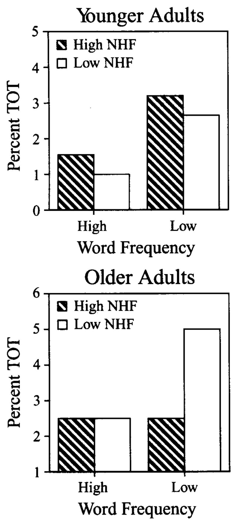
The percent of TOT responses as a function of word frequency and neighborhood frequency (NHF) for younger adults (top panel) and for older adults (bottom panel).
Age differences in TOT states
To examine age-related differences in TOTs, we combined the TOT data from Experiments 1 and 2. Although a number of findings reached statistical significance, for ease of exposition, only interactions involving the between-participants factor of age will be reported. A main effect of age was not statistically significant [F(1,45) = 1.78, p = .19], but there was a tendency for older adults (mean = 3.1 %) to report more TOT responses than younger adults (mean = 2.1%). Although not statistically significant, this trend is in the same direction as that reported by Burke et al. (1991) and James and Burke (2000) and may, as discussed earlier, reflect differences in the number of syllables in the stimuli used in the present versus previous studies.
No interaction of age and word frequency was found (F < 1). An interaction between age and density approached significance [F(1,45) = 4.08, p = .05]. For young adults, there was a tendency for more TOTs to be reported for words with sparse neighborhoods than for words with dense neighborhoods, but no difference was observed between the two conditions for older adults.
The interaction between age and neighborhood frequency also approached significance [F(1,45) = 4.04, p =.05]. Older adults tended to report more TOTs for words that had low neighborhood frequency (mean = 3.75%) than for words with high neighborhood frequency (mean = 2.5%). This trend was reversed for younger adults; more TOTs were reported for words that had high neighborhood frequency (mean = 2.4%) than for words with low neighborhood frequency (mean = 1.8%). Recall, however, that the main effects of neighborhood frequency were not significant for the young or older adults by themselves.
The interaction between age, word frequency, and neighborhood frequency, depicted in Figure 3, was also significant [F(1,45) = 4.64, p < .05]. For younger adults, the difference between words with high and low frequency was approximately equal for words with both high and low neighborhood frequency. However, for older adults the difference between the number of TOTs reported for high-and low-frequency words was much greater for words with low neighborhood frequency than for words with high neighborhood frequency.
Finally, an interaction was found between age, neighborhood density, and neighborhood frequency [F(1,45) = 5.28, p < .05]. As seen in Figure 4, younger adults consistently reported more TOTs for words with sparse neighborhoods than for words with dense neighborhoods, regardless of neighborhood frequency. In contrast, older adults tended to report more TOTs for words with sparse neighborhoods only when the word had low neighborhood frequency.
Figure 4.
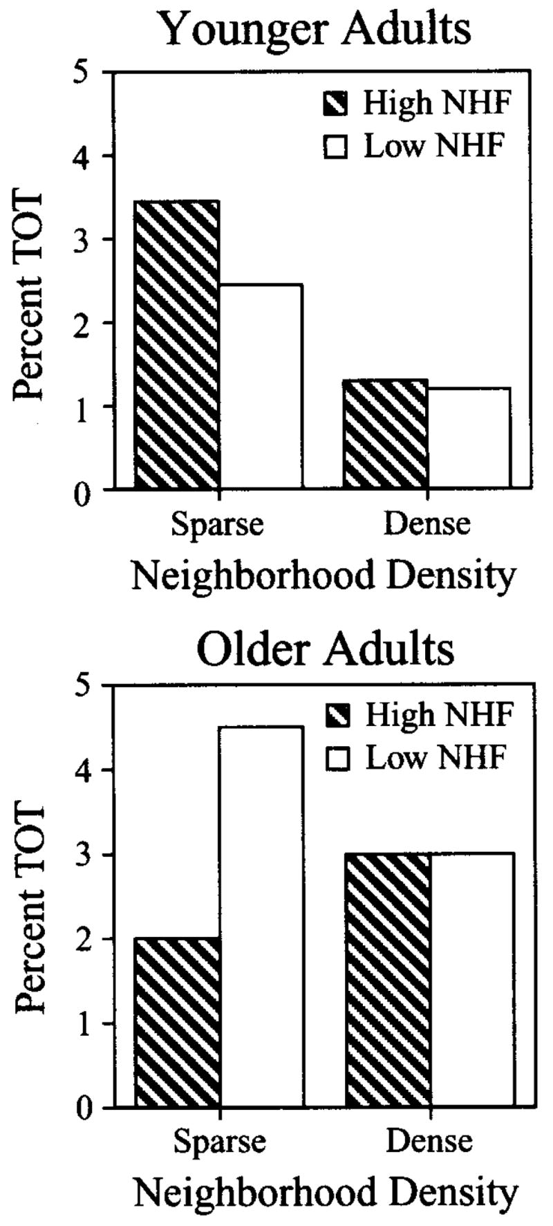
The percent of TOT responses as a function of density and neighborhood frequency (NHF) for younger adults (top panel) and for older adults (bottom panel).
Discussion
The results of the present experiment replicate and extend the results of a number of previous experiments investigating the TOT phenomenon in younger and older adults. Specifically, we found that older adults responded “know” more often than younger adults, “don’t know” fewer times than younger adults, and tended to report more TOT states than younger adults, replicating findings by Burke et al. (1991; see also Burke & Laver, 1990; James & Burke, 2000; MacKay & Burke, 1990; Rastle & Burke, 1996).
More importantly, we report a novel finding in this experiment: Older adults exhibited significantly more TOT states for words with low neighborhood frequency (if those words were also low-frequency words or words with sparse neighborhoods) than for words with high neighborhood frequency. To our knowledge, this is the first experiment to demonstrate significant effects of neighborhood frequency on speech production (see Vitevitch, 1997,2002). To better demonstrate that neighborhood frequency affects the process of lexical retrieval in speech production (rather than the failure to retrieve an item, as occurs during the TOT state), a picture-naming task was used in Experiment 3.
EXPERIMENT 3
An important aim of our study was to demonstrate neighborhood density and neighborhood frequency effects in the TOT task—a task that has played a central role in the debate regarding the influence of phonologically related words in speech production—but we also wanted to demonstrate that these two variables more directly influence lexical retrieval in speech production. Rather than demonstrate that these variables influence the inability to retrieve a lexical item (i.e., the TOT state), Experiment 3 used a picture-naming task to directly show that neighborhood frequency influences lexical retrieval in speech production (see Levelt, Roelofs, & Meyer, 1999, for the importance of on-line tasks in speech production studies). Given the processing advantage observed in Experiment 2 for high neighborhood frequency (i.e., participants exhibited fewer TOTs), it was predicted that participants would more quickly name pictures illustrating words that had high neighborhood frequency than pictures illustrating words that had low neighborhood frequency.
Method
Participants
Twenty-one older participants from the same population sampled in Experiment 2 took part in this experiment.
Materials
Line drawings (from Snodgrass & Vanderwart, 1980) for 54 monosyllabic CVC words were used as stimuli in the present experiment. Half of the line drawings illustrated words with high neighborhood frequency, and the other half illustrated words with low neighborhood frequency. Equal numbers of words in each condition contained the same initial phonemes. We used the same database as in Experiments 1 and 2; the words with high neighborhood frequency had a significantly higher mean frequency for the neighbors (mean = 222 occurrences per million) than the words with low neighborhood frequency (mean = 56 occurrences per million) [F(1,52) = 50.42, MSe = 372,802, p < .001].
Although the difference in neighborhood frequency of the two conditions was significant, the differences in familiarity ratings, word frequency, neighborhood density, and phonotactic probability (Vitevitch, 2002; Vitevitch & Luce, 1998, 1999) were not [all Fs(1,52) < 1 ]. Words with high neighborhood frequency had a mean familiarity rating of 6.95, a mean frequency of 41 occurrences per million, and a mean neighborhood density of 16 words. Phonotactic probability was assessed by the sum of the biphones and the sum of the phonemes making up the word, as in Vitevitch (2002; see also Vitevitch & Luce, 1998, 1999). The sum of the biphones = .008, and the sum of the phonemes = . 165 for words with high neighborhood frequency. In comparison, words with low neighborhood frequency had a mean familiarity rating of 6.84, a mean frequency of 36 occurrences per million, and a mean neighborhood density of 15 words. The sum of the biphones = .007, and the sum of the phonemes = .152 for words with low neighborhood frequency.
Finally, previous research has shown that normal and patient populations name pictures of living objects more quickly and accurately than pictures of nonliving objects (e.g., Kiefer, 2001; Laws, Leeson, & Gale, 2002; Takarae & Levin, 2001). For words with high neighborhood frequency there were 11 objects of organic origin (deer, foot, goat, hive, leg, log, nose, pear, run, seal, and sheep) and 16 inorganic objects (bib, bike, book, bus, cage, cake, cape, chair, comb, cone, cup, fan, kite, knife, pan, pen). For words with low neighborhood frequency there were 10 objects of organic origin (bird, bull, duck, face, goose, hawk, leaf, lip, neck, peach) and 17 inorganic objects (bell, bowl, cape, cave, chain, coach, coat, cog, couch, cuff, file, nail, pick, pole, ring, shirt, sock). A two-way chi-square analysis confirmed there was no difference between the two conditions with regard to the number of living and nonliving objects [x2 — (1, n= 54) = 0.08, n.s.]. Furthermore, 20 undergraduate students at the University of Kansas rated how well the words used to label the pictures described the objects on a scale from 1 (does not describe the picture well) to 7 (describes the picture well). A repeated measures ANOVA confirmed there was no difference between the two conditions in how well the words described the objects [F(1,19) < 1 ]. Words with low neighborhood frequency had a mean rating of 6.3, and words with high neighborhood frequency had a mean rating of 6.4.
Procedure
Participants studied a booklet that, on each page, contained the stimulus picture and the monosyllabic word that identified that picture. Previewing the picture and the word served to attenuate potential differences in the recency with which participants encountered these words (Burke et al., 1991). When participants were confident that they could use the given label for each picture, they were seated in front of an iMac running PsyScope 1.2.2 (Cohen, MacWhinney, Flatt, & Provost, 1993), which controlled stimulus randomization and presentation and collection of response latencies. A headphone-mounted microphone (Beyer-Dynamic DT109) was interfaced to a PsyScope button box that acted as a voice-key with millisecond accuracy. A typical trial proceeded as follows: The word “ready” appeared in the center of the monitor for 500 msec. One of the 54 randomly selected stimulus pictures was then presented and remained visible until a verbal response was initiated. Response latency, measured from the beginning of the stimulus, was triggered by the onset of the participant’s verbal response. Another trial began 1 sec after a response was made. Responses were also recorded on high-quality audiotape for later accuracy analyses. No picture was presented more than once.
Results
Only accurate responses were included in the repeated measures ANOVA for response latency. Responses other than the given label (e.g., responding with “sofa” instead of “couch”) were counted as errors. Responses that improperly triggered the voice-key (e.g., cough, “uh,” etc.) were not included in the analyses (and accounted for less than 1% of incorrect responses). Participants responded to words with high neighborhood frequency more quickly (876 msec) than to words with low neighborhood frequency (937 msec) [F(1,20) = 31.19, p < .001]. Participants also produced words with high neighborhood frequency more accurately (87.3%) than they did words with low neighborhood frequency (78.2%) [F(1,20) = 28.95, p<.001].
Discussion
The results of the picture-naming task in the present experiment provided additional evidence for a processing advantage for words with high frequency neighborhoods. Specifically, words with high frequency neighborhoods were produced more quickly and accurately than words with low frequency neighborhoods. The results of the present experiment, together with the results of Vitevitch (2002), suggest that multiple word forms are activated in memory and do influence the speed and accuracy of speech production. More importantly, the frequency of occurrence of the partially activated neighbors also influences the processes involved in speech production.
Interestingly, the neighborhood density and neighborhood frequency effects observed in the present set of speech production experiments were facilitative rather than competitive, as is often observed in speech perception. That is, in speech perception a word with a sparse neighborhood is retrieved more quickly and accurately than a word with a dense neighborhood (Luce & Pisoni, 1998; Vitevitch & Luce, 1998, 1999). A word with high neighborhood frequency is retrieved more slowly and less accurately than a word with low neighborhood frequency (Luce & Pisoni, 1998). These results are exactly the opposite of the processing advantages observed in the present set of experiments for words with high neighborhood frequency and density. These findings may further guide modeling efforts in speech production and speech perception, especially those efforts attempting to describe the nature of the architecture (i.e., feedforward vs. interactive) and those efforts attempting to model the interface between speech production and speech perception (e.g., NST; MacKay, 1987).
GENERAL DISCUSSION
The present set of experiments has resulted in a number of important new findings in the field of speech production. First, the TOT elicitation task was successfully used with highly familiar monosyllabic words instead of the unique multisyllabic words typically employed in TOT elicitation experiments, further suggesting that the TOT phenomenon is a failure of the same retrieval processes used to access words during the fluent production of speech. Second, we demonstrated an influence of neighborhood density in the context of the TOT phenomenon (which was not confounded by an orthographic measure of similarity or word length; see Harley & Bown, 1998). That is, neighborhood density not only influences naturalistic retrieval errors (Vitevitch, 1997), induced speech errors, and online picture naming (Vitevitch, 2002), but also influences those situations in which lexical retrieval fails (see also Dell & Gordon, in press; Gordon, 2002; Gordon & Dell, 2001). Furthermore, this is the first demonstration of the influence of neighborhood density (interacting with word and neighborhood frequency) in speech production in older adults. Finally, we experimentally demonstrated a novel influence of neighborhood frequency on the speed and accuracy of lexical retrieval during speech production. This unique empirical observation is also a novel finding in older adults.
How might a model of speech production account for the facilitative effects of neighborhood density and neighborhood frequency observed in part in Vitevitch (2002) and in the present set of experiments? In Dell’s (1986) interactive model of speech production (indeed, in most models of speech production) there are no lateral connections between representations within a level. Without lateral connections between similar sounding word forms, an interactive model of speech production can still account for the facilitative effects of neighborhood density in the following way. When the representation of a word form (cat) is partially activated by semantic information, the word form will partially activate the phonological nodes that constitute it (/k/ /æ/ /t/). (Note that in an interactive model other word forms may be partially activated by semantic information, but for ease of explication, we will only follow the activation of cat.) The activated phonological nodes (/k/ /æ/ /t/) will feed activation back to the word-form level to all the word forms that contain those phonemes (e.g., hat, cut, cap, etc.). The partially activated neighbors in turn send activation back down to the phonological nodes, thereby increasing the activation of those shared phonological nodes.
The amount of activation that the shared phonological nodes receive from the partially activated neighbors will depend on the number of neighbors as well as the frequency of occurrence of the neighbors. The activation received by the shared phonological nodes from the neighbors will in turn spread back to the target word and will increase the probability that the target word (being the highest activated representation) will be selected.
Consider a target word with a dense neighborhood. Such a word will receive greater amounts of activation via the shared phonological nodes than a target word with a sparse neighborhood because of the difference in the number of similar words contributing to the activation of the shared phonological nodes. The greater amount of activation from the larger number of neighbors will result in words with dense neighborhoods being produced faster and more accurately than words with sparse neighborhoods (Dell & Gordon, in press; Gordon, 2002; Gordon & Dell, 2001; Vitevitch, 2002).
Now consider a target word with high neighborhood frequency. Such a word will receive greater amounts of activation via the shared phonological nodes than a target word with low neighborhood frequency because the high-frequency neighbors will be slightly more active than the low-frequency neighbors. The greater amount of activation from the high-frequency neighbors will contribute a greater amount of activation to the shared phonological nodes and will result in words with high neighborhood frequency being produced faster and more accurately than words with low neighborhood frequency, as observed in the present experiments.
In contrast, it is unclear how a strictly feedforward model of speech production, such as WEAVER+ + (Levelt et al., 1999), could account for the present set of results. In WEAVER+ + activation at the word-form level can not spread “backward” to influence the activation of a lemma, nor can activation among phonological segments spread “backward” to influence the activation of word forms. The only “feedback” in WEAVER+ + is indirectly through the speech comprehension system, which is not considered feedback in the traditional sense. Even if we grant “feedback” through the speech comprehension system, it is unclear how this mechanism could account for the results of the present set of experiments. Recall that Luce and Pisoni (1998) found competitive effects of neighborhood density in spoken word recognition: Words with sparse neighborhoods were recognized more quickly and accurately than words with dense neighborhoods. Luce and Pisoni also found that words with low neighborhood frequency were recognized more quickly and accurately than words with high neighborhood frequency. Note that the perceptual results of Luce and Pisoni are exactly the opposite of those observed in the present set of production experiments. It is not at all clear how “feedback” through the (rather unspecified) speech comprehension system in WEAVER + + would enable a poorly perceived word with a dense neighborhood, for example, to then be produced more quickly and accurately.
Levelt et al. (1999) discussed how WEAVER + + could account for some facilitative effects reported in the literature. However, they discussed, in Section 5.2.1, facilitative effects among words that are semantically related rather than phonologically related. It is unclear whether the same mechanisms would also apply to phonological word forms. The discussion in Section 6.4 of Levelt et al. (1999; see also Meyer & Schriefers, 1991; Roelofs, 1997) actually suggests a slightly different mechanism to account for facilitative effects among phonologically related items. It is important to note, however, that the facilitative effects they discussed were obtained using the picture-word interference task. The picture-word interference task is essentially a priming task, in which a picture is presented visually and a word is presented (typically) auditorily at various stimulus onset asynchronies. Work by Roediger et al. (1983; see also Bowles & Poon, 1985, among others) showed that the relationship between the prime and the target in priming tasks may induce task-specific retrieval strategies, which may not reflect the strategies used during normal processing. The fact that Levelt et al. (1991) found inhibitory effects of phonologically overlapping primes and targets when lexical decisions were made to the auditory primes lends credence to the possibility that the facilitative effects obtained with the picture-word interference task may be task-specific artifacts. Most importantly, the facilitative effects in the picture-word interference task occurred for the subsequently presented word (i.e., the target) that was phonologically related to the previously presented item (i.e., the prime). It is not clear whether the mechanism in WEAVER + + that accounts for the facilitative effects in the picture-word interference task can also account for the facilitative effects obtained for phonologically related words that are simultaneously activated during speech production (i.e., neighbors), as observed in the present set of experiments.
Without feedback from the phonological level to the word forms, or without lateral connections among word forms, it is unclear how phonological neighbors may even be activated at all in the strictly feedforward architecture of WEAVER+ +. Levelt et al. (1999; see also Roelofs, 1992) did suggest that multiple word forms may be activated in situations in which two (or presumably more) lemmas are equally activated and selected. However, given the arbitrary relationship between meaning and sound (e.g., Saussure, 1966), it is unlikely that these semantically related representations would also be phonologically related (e.g., sofa and couch). If there is no mechanism in WE AVER++ to activate phonological neighbors (and possibly account for the neighborhood density effects observed in this and other studies), then there is also no way to account for the influence of the frequency of those neighbors, as demonstrated in the present set of experiments. In short, accounting for the several novel findings observed in younger and older adults in the present set of experiments may prove to be challenging for certain models of speech production.
Acknowledgments
This research was supported in part by Training Grant DC 00012 (to Indiana University while M.S.V. was a postdoctoral researcher) and Research Grant DC 04259 (to Indiana University and the University of Kansas) from the National Institute on Deafness and Other Communication Disorders, National Institutes of Health, and a grant from the Brookdale Foundation (to Washington University). We thank Emily Mc-Cutcheon and Shinying Chu for their assistance in data collection and analysis, Luis R. Hernandez for his programming assistance, and three anonymous reviewers for their helpful comments and suggestions.
Contributor Information
MICHAEL S. VITEVITCH, University of Kansas, Lawrence, Kansas
MITCHELL S. SOMMERS, Washington University, St. Louis, Missouri
References
- Bard E, Shillcock R. Competitor effects during lexical access: Chasing Zipf’s tail. In: Altmann G, Shillcock R, editors. Cognitive models of speech processing. Hove, U.K.: Erlbaum; 1993. pp. 235–275. [Google Scholar]
- Bowles NL, Poon LW. Effects of priming in word retrieval. Journal of Experimental Psychology: Learning, Memory, & Cognition. 1985;11:272–283. doi: 10.1037//0278-7393.11.2.272. [DOI] [PubMed] [Google Scholar]
- Brennen T, Baguley T, Bright J, Bruce V. Resolving semantically induced tip-of-the-tongue states for proper nouns. Memory & Cognition. 1990;18:339–347. doi: 10.3758/bf03197123. [DOI] [PubMed] [Google Scholar]
- Brown AS. A review of the tip-of-the-tongue experience. Psychological Bulletin. 1991;109:204–223. doi: 10.1037/0033-2909.109.2.204. [DOI] [PubMed] [Google Scholar]
- Brown R, McNeill D. The “tip of the tongue” phenomenon. Journal of Verbal Learning & Verbal Behavior. 1966;5:325–337. [Google Scholar]
- Burke DM, Laver GD. Aging and word retrieval: Selective age deficits in language. In: Lovelace EA, editor. Aging and cognition: Mental processes, self-awareness and interventions. Amsterdam: Elsevier, North-Holland; 1990. pp. 281–300. [Google Scholar]
- Burke DM, Mackay DG, Worthley JS, Wade E. On the tip of the tongue: What causes word finding failures in young and older adults? Journal of Memory & Language. 1991;30:542–579. [Google Scholar]
- Cohen JD. Random means random. Journal of Verbal Learning & Verbal Behavior. 1976;15:261–262. [Google Scholar]
- Cohen JD, Macwhinney B, Flatt M, Provost J. PsyScope: An interactive graphic system for designing and controlling experiments in the psychology laboratory using Macintosh computers. Behavioral Research Methods, Instruments, & Computers. 1993;25:257–271. [Google Scholar]
- Coltheart M, Davelaar E, Jonasson JT, Besner D. Access to the internal lexicon. In: Dornic S, editor. Attention and performance VI. London: Academic Press; 1977. pp. 535–555. [Google Scholar]
- Dell GS. A spreading-activation theory of retrieval in sentence production. Psychological Review. 1986;93:283–321. [PubMed] [Google Scholar]
- Dell GS, Gordon JK. Neighbors in the lexicon: Friends or foes? In: Schiller NO, Meyer AS, editors. Phonetics and phonology in language comprehension and production: Differences and similarities. New York: Mouton de Gruyter; in press. [Google Scholar]
- Godden D, Baddeley AD. Context-dependent memory in two natural environments: On land and under water. British Journal of Psychology. 1975;66:325–331. [Google Scholar]
- Gordon JK. Phonological neighborhood effects in aphasic speech errors: Spontaneous and structured contexts. Brain & Language. 2002;82:113–145. doi: 10.1016/s0093-934x(02)00001-9. [DOI] [PubMed] [Google Scholar]
- Gordon JK, Dell GS. Phonological neighbourhood effects: Evidence from aphasia and connectionist modeling. Brain & Language. 2001;79:21–23. [Google Scholar]
- Harley TA, Bown HE. What causes a tip-of-the-tongue state? Evidence for lexical neighbourhood effects in speech production. British Journal of Psychology. 1998;89:151–174. [Google Scholar]
- Hino Y, Lupker SJ. Effects of word frequency and spelling-to-sound regularity in naming with and without preceding lexical decision. Journal of Experimental Psychology: Human Perception & Performance. 2000;26:166–183. doi: 10.1037//0096-1523.26.1.166. [DOI] [PubMed] [Google Scholar]
- James LE, Burke DM. Phonological priming effects on word retrieval and tip-of-the-tongue experiences in young and older adults. Journal of Experimental Psychology: Learning, Memory, & Cognition. 2000;26:1378–1391. doi: 10.1037//0278-7393.26.6.1378. [DOI] [PubMed] [Google Scholar]
- Jones GV. Back to Woodworth: Role of interlopers in the tip-of-the-tongue phenomenon. Memory & Cognition. 1989;17:69–76. doi: 10.3758/bf03199558. [DOI] [PubMed] [Google Scholar]
- Jones GV, Langford S. Phonological blocking in the tip of the tongue state. Cognition. 1987;25:115–122. doi: 10.1016/0010-0277(87)90027-8. [DOI] [PubMed] [Google Scholar]
- Keppel G. Words as random variables. Journal of Verbal Learning & Verbal Behavior. 1976;15:263–265. [Google Scholar]
- Kiefer M. Perceptual and semantic sources of category-specific effects: Event-related potentials during picture and word categorization. Memory & Cognition. 2001;29:100–116. doi: 10.3758/bf03195745. [DOI] [PubMed] [Google Scholar]
- Kuèera H, Francis WN. Computational analysis of present-day American English. Providence, RI: Brown University Press; 1967. [Google Scholar]
- Landauer TK, Streeter LA. Structural differences between common and rare words: Failure of equivalence assumptions for theories of word recognition. Journal of Verbal Learning & Verbal Behavior. 1973;12:119–131. [Google Scholar]
- Laws KR, Leeson VC, Gale TM. The effect of “masking” on picture naming. Cortex. 2002;38:137–148. doi: 10.1016/s0010-9452(08)70646-4. [DOI] [PubMed] [Google Scholar]
- Levelt WJM. Speaking: From intention to articulation. Cambridge, MA: MIT Press; 1989. [Google Scholar]
- Levelt WJM, Roelofs A, Meyer AS. A theory of lexical access in speech production. Behavioral & Brain Sciences. 1999;22:1–38. doi: 10.1017/s0140525x99001776. [DOI] [PubMed] [Google Scholar]
- Levelt WJM, Schriefers H, Vorberg D, Meyer AS, Pech-Mann T, Havinga J. The time course of lexical access in speech production: A study of picture naming. Psychological Review. 1991;98:122–142. [Google Scholar]
- Luce PA, Pisoni DB. Recognizing spoken words: The neighborhood activation model. Ear & Hearing. 1998;19:1–36. doi: 10.1097/00003446-199802000-00001. [DOI] [PMC free article] [PubMed] [Google Scholar]
- MacKay DG. The organization of perception and action: A theory for language and other cognitive skills. New York: Springer-Verlag; 1987. [Google Scholar]
- MacKay DG, Burke DM. Cognition and aging: A theory of new learning and the use of old connections. In: Hess TM, editor. Aging and cognition: Knowledge organization and utilization. Amsterdam: Elsevier, North-Holland; 1990. pp. 213–263. [Google Scholar]
- Marslen-Wilson WD, Zwitserlood P. Accessing spoken words: The importance of word onsets. Journal of Experimental Psychology: Human Perception & Performance. 1989;15:576–585. [Google Scholar]
- Maylor EA. Age, blocking and the tip of the tongue state. British Journal of Psychology. 1990;81:123–134. doi: 10.1111/j.2044-8295.1990.tb02350.x. [DOI] [PubMed] [Google Scholar]
- McClelland JL, Elman JL. The TRACE model of speech perception. Cognitive Psychology. 1986;18:1–86. doi: 10.1016/0010-0285(86)90015-0. [DOI] [PubMed] [Google Scholar]
- Meyer AS, Bock JK. The tip-of-the-tongue phenomenon: Blocking or partial activation? Memory & Cognition. 1992;20:715–726. doi: 10.3758/bf03202721. [DOI] [PubMed] [Google Scholar]
- Meyer AS, Schriefers H. Phonological facilitation in picture-word interference experiments: Effects of stimulus onset asynchrony and types of interfering stimuli. Journal of Experimental Psychology: Learning, Memory & Cognition. 1991;17:1146–1160. [Google Scholar]
- Murphy KR, Myors B. Statistical power analysis: A simple and general model for traditional and modern hypothesis tests. Mahwah, NJ: Erlbaum; 1998. [Google Scholar]
- Norris D, Mcqueen JM, Cutler A. Merging information in speech recognition: Feedback is never necessary. Brain & Behavioral Sciences. 2000;23:299–370. doi: 10.1017/s0140525x00003241. [DOI] [PubMed] [Google Scholar]
- Nusbaum HC, Pisoni DB, Davis CK. Sizing up theHoosier mental lexicon: Measuring the familiarity of 20,000 words (Research on Speech Perception Progress Report No. 10) Bloomington: Indiana University, Department of Psychology, Speech Research Laboratory; 1984. [Google Scholar]
- Perfect TJ, Hanley JR. The tip-of-the-tongue phenomenon: Do experimenter-presented interlopers have any effect? Cognition. 1992;45:55–75. doi: 10.1016/0010-0277(92)90023-b. [DOI] [PubMed] [Google Scholar]
- Pisoni DB, Nusbaum HC, Luce PA, Slowiaczek LM. Speech perception, word recognition and the structure of the lexicon. Speech Communication. 1985;4:75–95. doi: 10.1016/0167-6393(85)90037-8. [DOI] [PMC free article] [PubMed] [Google Scholar]
- Raaijmakers JGW, Schrijnemakers JMC, Gremmen F. How to deal with “the language-as-fixed-effect fallacy”: Common misconceptions and alternative solutions. Journal of Memory & Language. 1999;41:416–426. [Google Scholar]
- Rastle KG, Burke DM. Priming the tip of the tongue: Effects of prior processing on word retrieval in young and older adults. Journal of Memory & Language. 1996;35:586–605. [Google Scholar]
- Riefer DM, Keveri MK, Kramer DLF. Name that tune: Eliciting the tip-of-the-tongue experience using auditory stimuli. Psychological Reports. 1995;77:1379–1390. doi: 10.2466/pr0.1995.77.3f.1379. [DOI] [PubMed] [Google Scholar]
- Roediger HL, III, Neely JH, Blaxton TA. Inhibition from related primes in semantic memory retrieval: A reappraisal of Brown’s (1979) paradigm. Journal of Experimental Psychology: Learning, Memory, & Cognition. 1983;9:478–485. [Google Scholar]
- Roelofs A. A spreading-activation theory of lemma retrieval in speaking. Cognition. 1992;42:107–142. doi: 10.1016/0010-0277(92)90041-f. [DOI] [PubMed] [Google Scholar]
- Roelofs A. The WEAVER model of word-form encoding in speech production. Cognition. 1997;64:249–284. doi: 10.1016/s0010-0277(97)00027-9. [DOI] [PubMed] [Google Scholar]
- Saussure FDe. In: Course in general linguistics. Baskin Wade., translator. New York: McGraw-Hill; 1966. (Original work presented 1916) [Google Scholar]
- Schacter DL. The seven sins of memory: Insights from psychology and cognitive neuroscience. American Psychologist. 1999;54:182–203. doi: 10.1037//0003-066x.54.3.182. [DOI] [PubMed] [Google Scholar]
- Smith JEK. The assuming-will-make-it-so fallacy. Journal of Verbal Learning & Verbal Behavior. 1976;15:262–263. [Google Scholar]
- Smith SM, Brown JM, Balfour SP. TOTimals: A controlled experimental method for studying tip-of-the-tongue states. Bulletin of the Psychonomic Society. 1991;29:445–447. [Google Scholar]
- Snodgrass JG, Vanderwart M. A standardized set of 260 pictures: Norms for name agreement, image agreement, familiarity, and visual complexity. Journal of Experimental Psychology: Human Learning & Memory. 1980;6:174–215. doi: 10.1037//0278-7393.6.2.174. [DOI] [PubMed] [Google Scholar]
- Takarae Y, Levin DT. Animals and artifacts may not be treated equally: Differentiating strong and weak forms of category-specific visual agnosia. Brain & Cognition. 2001;45:249–264. doi: 10.1006/brcg.2000.1244. [DOI] [PubMed] [Google Scholar]
- Vitevitch MS. The neighborhood characteristics of malapropisms. Language & Speech. 1997;40:211–228. doi: 10.1177/002383099704000301. [DOI] [PubMed] [Google Scholar]
- Vitevitch MS. The influence of phonological similarity neighborhoods on speech production. Journal of Experimental Psychology: Learning, Memory, & Cognition. 2002;28:735–747. doi: 10.1037//0278-7393.28.4.735. [DOI] [PMC free article] [PubMed] [Google Scholar]
- Vitevitch MS, Luce PA. When words compete: Levels of processing in spoken word perception. Psychological Science. 1998;9:325–329. [Google Scholar]
- Vitevitch MS, Luce PA. Probabilistic phonotactics and spoken word recognition. Journal of Memory & Language. 1999;40:374–408. [Google Scholar]
- Webster’s New Collegiate Dictionary. Springfield, MA: Merriam; 1979. [Google Scholar]
- Wike EL, Church JD. Comments on Clark’s “The language-as-fixed-effect-fallacy. Journal of Verbal Learning & Verbal Behavior. 1976;15:249–255. [Google Scholar]
- Woodworth RS. Psychology. 2. New York: Holt; 1929. [Google Scholar]
- Yarmey AD. I recognize your face but I can’t remember your name: Further evidence on the tip-of-the-tongue phenomenon. Memory & Cognition. 1973;1:287–290. doi: 10.3758/BF03198110. [DOI] [PubMed] [Google Scholar]
- Zipf GK. The psycho-biology of language: An introduction to dynamic philology. Cambridge, MA: Houghton Mifflin; 1935. [Google Scholar]