Time Course of Information about Motion Direction in Visual Area MT of Macaque Monkeys

Abstract

We used the responses of neurons in extrastriate visual area MT to determine how well neural noise can be reduced by averaging the responses of neurons across time. For individual MT neurons, we calculated the time course of Shannon information about motion direction from sustained motion at constant velocities. Stimuli were random dot patterns moving at the preferred speed of the cell for 256 msec, in a direction chosen randomly with 15° increments. Information about motion direction calculated from cumulative spike count rose rapidly from the onset of the neural response and then saturated, reaching 80% of maximum information in the first 100 msec. Most of the early saturation of information could be attributed to correlated fluctuations in the spike counts of individual neurons on time scales in excess of 100 msec. Thus, temporal correlations limit the benefits of averaging across time, much as correlations among the responses of different neurons limit the benefits of averaging across large populations. Although information about direction was available quickly from MT neurons, the direction discrimination by individual MT neurons was poor, with mean thresholds above 30° in most neurons. We conclude that almost all available directional information could be extracted from the first few spikes of the response of the neuron, on a time scale comparable with the initiation of smooth pursuit eye movements. However, neural responses still must be pooled across the population in MT to account for the direction discrimination of the pursuit behavior.

Introduction

Our understanding of the neural code should be both informed and constrained by the time scales of relevance for animal behavior. In flies, for example, we know that visual motion can trigger flight maneuvers in ∼30 msec (Land and Collett, 1974) and that visual motion can be represented on this time scale by short sequences of action potentials in motion-sensitive neurons (de Ruyter van Steveninck and Bialek, 1988; Rieke et al., 1997). Primate vision also guides both perceptual and motor behaviors that can occur over time scales of ∼100 msec, during which time only a few action potentials are fired by any given sensory neuron. Indeed, the 200 msec duration of most eye fixations implies that the visual system is capable of taking in sensory information on a short time scale, although most neurons in the mammalian visual cortex show sustained responses to visual stimuli.

Relatively little is known about how neural signals are integrated across time, especially by comparison with the large body of previous analyses of how they might be integrated across populations of neurons (Salinas and Abbott, 1994; Abbott et al., 1996; Shadlen et al., 1996; Oram et al., 1998; Abbott and Dayan, 1999; Pouget et al., 2000; Bair et al., 2001). Several previous papers have shown that reliable behavioral responses can be generated on a short time scale on the basis of relatively short exposures to visual stimuli (de Bruyn and Orban, 1988; Watamaniuk et al., 1989; Snowden and Braddick, 1991; Thorpe et al., 1996; Cook and Maunsell, 2002; Roitman and Shadlen, 2002; Gold and Shadlen, 2003). In addition, the discriminative power of neural responses may be excellent when based solely on the early transient component of longer sustained responses (Oram and Perrett, 1992; Tovee et al., 1993; Heller et al., 1995; Buracas et al., 1998; Muller et al., 2001; Palanca and DeAngelis, 2003). Our goal was to investigate the temporal scale of neural representation systematically in relation to a specific visually driven motor behavior.

Our analysis of how information is accumulated across time and populations of neurons is motivated by the time course over which visual motion guides smooth pursuit eye movements. Primates track small moving objects with smooth eye movements that depend on estimates of the speed and direction of target motion. The 100 msec latency from visual input to smooth eye movement output dictates that pursuit must be able to extract reliable estimates of image direction and speed on a time scale of 100 msec. We chose to focus on extrastriate area MT because it is a major source of the visual inputs that control pursuit (Newsome et al., 1985; Groh et al., 1997; Born et al., 2000) and because it projects, via the pontine nuclei, to the parts of the cerebellum that participate in pursuit eye movements (Giolli et al., 2001; Distler et al., 2002). Furthermore, neurons in MT have response properties that seem appropriate for guiding pursuit: they are selective for moving stimuli and are tuned for the direction and speed of visual motion (Maunsell and Van Essen, 1983). In the present paper, we show that MT neurons provide a burst of information about motion direction on the 100 msec time scale needed to drive pursuit behavior and that this information is carried by just a handful of spikes. Still, the precision of pursuit behavior requires pooling information from many individual neurons.

Materials and Methods

Physiological preparation. Extracellular single-unit microelectrode recordings were made in area MT of three anesthetized, paralyzed macaque monkeys (Macaca fasicularis). Surgery, monitoring, and preparations for electrophysiological recording were performed using methods described by Priebe et al. (2002). Briefly, anesthesia was induced with ketamine (5–15 mg/kg) and midazolam (0.7 mg/kg) and continued under isofluorane (∼2%) and oxygen during surgical procedures. The animal's head was immobilized in a stereotaxic frame, a small craniotomy was performed directly above the superior temporal sulcus (STS), and a small portion of the dura was reflected to allow electrode penetration. After completion of the surgical procedures, anesthesia was maintained throughout the experiment with an intravenous opiate, sufentanil citrate (8–16 μg · kg^–1 · hr^–1). After a stable anesthetized state had been confirmed and followed for several hours, the paralytic agent vecuronium bromide (Norcuron, 0.1 mg · kg^–1 · hr^–1) was given intravenously to minimize eye movement. The electrocardiogram, electroencephalogram, autonomic signs, and rectal temperature were monitored continuously to ensure the anesthetic and physiological state of the animal. The upper eyelids were sutured to the stereotaxic frame to maximize the visual field. Pupils were dilated with topical atropine, and the corneas were protected with lubricated +2D gas-permeable lenses. Supplementary lenses were selected by direct opthalmoscopy to make the lens conjugate with the display. The locations of the foveae were recorded using a reversible opthalmoscope. Contact lenses were cleaned and relubricated, and the fovea was remapped as needed during the experiment.

We used a vertical approach to area MT. Tungsten-in-glass electrodes (Merrill and Ainsworth, 1972) were positioned by a hydraulic micromanipulator. After the electrode was in place, saline and agarose were placed over the craniotomy to protect the surface of the cortex and reduce movement of the brain. Electrodes were driven down through cortex on the anterior bank of the STS, across the lumen of the STS, and into area MT. Extracellular neural activity was amplified, bandpass filtered (100 Hz to 10 kHz), and displayed on a storage oscilloscope. Single units were isolated with a dual-window discriminator (DDIS-1; Bak Electronics, Germantown, MD).

Experiments lasted for ∼100–144 hr. The units included in this study are from three monkeys. The results of other experiments on the same neurons have been reported in a series of previous papers on other issues (Priebe and Lisberger, 2002; Priebe et al., 2002, 2003). The location of unit recordings in MT was confirmed by histological examination of the brain after the experiment as described by Lisberger and Movshon (1999). All methods had received previous approval by and were in compliance with the regulations of the Institutional Animal Care and Use Committee at University of California at San Francisco.

Stimulus presentation. Stimuli were presented on high-resolution analog display oscilloscopes (models 1304A and 1321B, P4 Phosphor; Hewlett-Packard, Palo Alto, CA) driven by a personal computer (PC)-based digital signal processing (DSP) board (“Detroit” system; Spectrum Signal Processing, Vancouver, Canada). The use of an analog oscilloscope afforded fast refresh rates (250 or 500 Hz), and the 16-bit digital-to-analog converters on the DSP board allowed 64,000 × 64,000 pixel resolution. Stimuli consisted of random dot textures moving through a square aperture in a field of stationary random dots. Both the moving and stationary textures had densities of 0.75 dots per square degree, and the virtual borders of the aperture were imperceptible when the center texture was stationary. Dot motion was coherent, with uniform velocity. After a single unit had been isolated in area MT, its receptive field was mapped by hand on a tangent screen. Once the location of the receptive field had been determined, we positioned a mirror so that the receptive field was centered on the video screen. The screen was 68 cm from the eye and subtended a 20° × 20° area. Stimuli were displayed monocularly. Experiments were performed in a dimly lit room. The background luminance of the display was <1 mcd/m². All MT neurons in our study had receptive fields that were centered within 10° of the fovea.

Experiments consisted of a sequence of brief trials with an intertrial interval of ∼700 msec. For all trials, both the surround and the center texture appeared and remained stationary for 256 msec. The center texture then moved at a constant velocity for 256 msec while the surround texture remained stationary. Both textures then remained stationary for another 256 msec before they were extinguished. When moving dots reached one edge of the window delineating the moving texture, they were extinguished and replaced by a new dot that appeared at a random location on the opposite border.

Before collecting the data needed to explore the time course of the representation of motion direction in MT, we conducted a series of experiments designed to optimize the visual stimulus for the receptive field of the neuron under study. First, we characterized the preferred direction of the cell by randomly interleaving trials that presented eight directions of motion. Second, we assessed the preferred speed of the cell with motion in the preferred direction at 11 speeds ranging from 0.125 to 128°/sec. Third, because the responses of neurons in MT can depend on the size of the moving texture (Allman et al., 1985), we optimized the size of the center patch of moving dots: we presented stimuli of the preferred direction and speed with motion in center textures that subtended 2.5°, 5°, 10°, 15°, or 20° and chose the aperture size that yielded the largest response. Finally, to confirm that the mirror was correctly centered on the receptive field of the neuron under study, the receptive field was mapped with 4° × 4° patches of dot motion of the preferred direction and speed. Often the last two steps of the stimulus optimization were iterated to ensure that the strongest response was being elicited from the MT neuron. Only those units that failed our isolation criteria were rejected from additional recording and analysis; as long as they responded to the moving dots, no units were rejected from our sample on the basis of response amplitude or directional tuning criteria.

To obtain the data analyzed in detail in this paper, we characterized direction selectivity on one of two finer grids of directions of motion. For 24 neurons, the directions of motion were ±90° relative to the preferred direction with a spacing of 15° (13 stimuli). For 12 neurons, we added directions on a 7.5° spacing at ±7.5° and ±52.5° relative to preferred direction (17 stimuli). The stimulus set also included a control trial that presented stationary dots. Stimuli were presented in blocks of trials, in which each block presented all stimuli in an experiment once, and the stimulus order was shuffled before each new block. Each stimulus was repeated up to 222 times for a given neuron. Dot placement within the texture was determined independently for each trial by starting with a new random seed.

Data acquisition and initial analysis. Experiments were controlled by a UNIX workstation (DEC Alpha). The workstation sent commands to a Pentium PC that both generated the stimuli and recorded the data. A hardware window discriminator was used to convert the action potentials to transistor–transistor logic (TTL) pulses, and the time of each TTL pulse was recorded by the computer with 10 μsec resolution. After each trial, data were sent via the local area network to the UNIX workstation and saved for later analysis along with a record of the commands given to generate the stimulus.

Data were analyzed using Matlab (MathWorks, Natick, MA). In preparation for the information theoretic analysis, the unit responses were sorted according to the direction of motion of the visual stimulus and aligned at stimulus appearance so that spikes could be counted in 2 msec bins for each stimulus. We used equal numbers of trials for each stimulus direction in all analyses. To compute transient/sustained ratio of firing rate, we corrected for background rate by subtracting the average spike count during the presentation of a stationary pattern from each average response (following Lisberger and Movshon, 1999) and then calculated the maximal response in a sliding 26 msec window within 170 msec of motion onset divided by the mean response in the interval from 156 to 256 msec after response onset.

To compute latency for analysis of the relationship between latency and direction of target motion, the neural responses were binned in 10 msec intervals, and the mean and SD of the background rate were computed from the response to the stationary dot pattern in the first 256 msec of each stimulus condition. Latency was taken as the first bin in the first run of four bins for which the response exceeded the background firing rate by two SDs (Raiguel et al., 1999). Although we began all information theoretic calculations at stimulus motion onset, we reference many of our measurements to the onset of the neural response to motion. To determine the response onset time, we averaged all responses to all directions of motion together and then marked response onset by eye. Because of the differences in the analysis method, the response onset time for the full set of stimuli differed slightly from the minimum latency for some units.

Information theoretic analysis. Our goal was to characterize not just the distributions of spike count themselves but rather the average extent to which the neural response allows us to identify the stimulus. We did this with information theory (Shannon and Weaver, 1949), by computing the information directly from the measured spike counts in different time intervals (T) as follows:

(1)

where:

(2)

I_count(T) quantifies in bits the amount of information that a single observation of the spike count, n, provides about the direction of motion, θ, and P_T(n) is the total probability of observing n spikes after counting over a time interval, T, averaged over all stimuli. In our case, all stimuli occurred with equal probability, P(θ).

We now give a brief, intuitive explanation of Equations 1 and 2. The mutual information between response and direction of motion is determined by quantifying the uncertainty, or variability, of the neural responses in units of bits by expressing them as an entropy. The entropy, S, of a probability distribution P(n) over a time interval T is given by the following:

(3)

The entropy of the response is the upper bound on the amount of information a cell can transmit about the stimulus, i.e., its coding capacity. Intuitively, the distribution of counts determines the number of different responses or “symbols” that the cell can use to encode aspects of the stimulus. The entropy of the count distribution is itself constrained by the average count: 〈n(T)〉. The higher the firing rate, the greater the range of counts that can be observed and, therefore, the more symbols available to encode the stimulus parameter. The maximal entropy can be expressed in terms of the average count at a given time (Rieke et al., 1997), as follows:

(4)

For each θ_i in our stimulus set, we expressed the variability of the neural response to repetitions of that stimulus, P(n θ_i), as a conditional entropy, S(P(n θ_i)), as in Equation 3. The amount by which recording a certain spike count, n, reduces our uncertainty about the direction of the stimulus, θ_i is the information gained in bits, or the difference between the entropies, as follows:

(5)

Computing I(θ_i) for each θ_i in our stimulus set yielded graphs like that shown in Figure 1 A. The mutual information then is the weighted average of the information over all stimuli, as follows:

(6)

Equation 6 expands to Equation 1.

Figure 1.

Methods for computing mutual information. A, Symbols connected by lines show the mean contribution of each stimulus direction to the mutual information as a function of stimulus direction for one MT neuron. The horizontal line shows the average information across direction. B, Extrapolation of information to remove the effects of finite data sets. Symbols show the information computed as a function of the inverse of the fraction of the data set used for the computation. The dashed line shows the result of linear regression analysis. Error bars show the SD obtained from bootstrapping with half of the data sample.

All analyses used a procedure to minimize the effects of finite sample size on our estimates of information. By randomly drawing different numbers of samples (N) from our total trial set for each neuron, we looked for the expected systematic behavior, as follows:

(7)

and extracted I_∞ as our best estimate following the methods of Strong et al. (1998) (see also Panzeri and Treves, 1996). The number of repeats in our dataset gave reasonable linear behavior keeping first-order terms in N only (Fig. 1 B). Note that the extrapolated estimate of information for an infinite dataset is always smaller than the value measured from a finite data set.

We computed information about direction (1) from cumulative spike count from the start of stimulus motion, (2) from spike counts in bins of different durations, and (3) on the basis of normalization for the number of spikes in the counting interval. For analysis of information per spike, the spike count was computed from the same trials used to compute information at each stage of the bootstrapping routine. If fewer than three spikes occurred in a given time window, so that the average count was less than three divided by the total number of trials, then the information per spike was set to zero. Error bars for all quantities were obtained by computing the SD of information computed from bootstrapping with half of the total trials. We confirmed that analysis of synthetic data in which trials had been randomized with respect to stimulus identity yielded estimates of information that were not statistically different from zero.

Other forms of data analysis. To analyze the autocorrelation of the spiking within trials, we computed the “shuffle-corrected” correlation function of the spike trains, corresponding to what is known in physics as the “connected” correlation function for time lags from 2 to 500 msec. For each trial, we binned the 768-msec-long spike trains in 2 msec bins, including the data from the intervals when the visual stimulus was both stationary and moving. The autocorrelation of the number of spikes per bin was computed from all of the trials for a given motion direction by computing the within-trial correlation both forward and backward in time for each time point in each trial and then averaging across all trials. If the start point for a given lag time was <500 msec from the end or start of the trials, then only the available bins were included in the average, yielding a different number of samples for each lag. To compute the shuffle-corrected correlation function of the spike trains, we computed the autocorrelation function of the spike trains within each trial, averaged over trials, and subtracted the autocorrelation function of the average time-dependent firing rate. The analysis was done separately for each direction of motion. We smoothed the functions with a sliding 20 msec window and normalized separately for the average firing rate in each direction, so that the correlation function can be interpreted as a conditional firing rate and has units of spike per second (Rieke et al., 1997, their Appendix A.2). We used bootstrapping to estimate error bars for the autocorrelograms: SDs were computed for autocorrelations computed from random draws of half of the trials.

To further assess the statistical significance of the connected (shuffle-corrected) autocorrelation function, we performed the same calculations on time-shuffled or “synthetic Poisson” spike trains for each neuron. These were generated by drawing the value of count in each 2 msec time bin randomly from the set of all responses in that bin for all trials that presented the same direction of motion. The resulting synthetic spike trains have the same average time-dependent firing rate as the real neuron, but no other correlations across time, so that they are equivalent to an inhomogeneous, or time-dependent, Poisson process. In particular, the spike counts in non-overlapping time windows will fluctuate independently around mean values determined by the time-dependent firing rate. Finally, we analyzed the discriminability of direction for each MT neuron by computing the information about direction for all pairs of directions in our stimulus set. Pairs of stimuli differed by angles that ranged from a minimum of 7.5° or 15° to 180°. To relate the information about direction to the “percent correct” measure (Green and Swets, 1966) that is traditionally used to report discrimination in two-alternative forced-choice paradigms, we used the following equation:

(8)

If we assume symmetric error probabilities in misidentifying two stimuli, then Equation 8 describes the relationship between mutual information in bits (I) and probability of a correct choice or percentage correct, (P_c) for a pair of stimuli. The estimate of (P_c) obtained with this approach is an upper bound on the actual probability of a correct choice, computable by signal detection theory (receiver operating characteristic or ROC analysis) for two conditional probability distributions of any shape (Green and Swets, 1966).

Results

Properties of averaged responses

MT neurons respond to steps of stimulus speed with a time-varying firing rate whose average shape and onset timing depends on motion direction. For stimuli moving at or near the preferred direction (Fig. 2A), the response is often characterized by a high spike rate transient followed by a lower sustained response (Lisberger and Movshon, 1999). As the direction of the stimulus is varied, the average response amplitude and the latency of the response both vary (Fig. 2B). Responses are stronger, and variability of the spike count highest, for motion in the preferred direction. Both are smaller for stimuli moving in nonpreferred directions (Fig. 2C). The average firing rate during the response to preferred direction texture motion for our sample ranged from 4 to 163 spikes/sec with a mean of 45 spikes/sec. The latency of the response tends to be shortest for directions near the preferred direction and increases as a function of the difference between direction of motion and preferred direction. As shown in Figure 2D, the amount of increase in latency ranged across the population: stimuli that moved in a direction 45° from the preferred direction caused responses at latencies that were 10–140 msec longer than for motion in the preferred direction: mean and median increments in latency were 37 and 20 msec. The rare examples of very long latencies result from the application of an objective latency measurement to weak responses and do not reflect “off responses” to motion in nonpreferred directions, which are rare in MT neurons. Our data on the direction tuning of response amplitude and latency agree with previous studies of MT (Maunsell and Van Essen, 1983; Raiguel et al., 1999).

Figure 2.

Directional responses of MT neurons. A–C show data from the same neuron. A, Top to bottom, The rasters show the responses to 184 repetitions of the same stimulus, the trace labeled “speed” shows the time course of the step of stimulus speed, and the trace labeled “Firing rate” shows the average response for all 184 repetitions. Stimulus was at the preferred speed, direction was 15° from preferred direction, and the duration of the target motion was 256 msec. B, Time course of mean firing rates for 13 directions of stimulus motion. The asterisk indicates the direction shown in A. C, Direction tuning of the total spike count in the interval from 0 to 256 msec after the start of the response to stimulus motion. Error bars show SDs. D, Effect of stimulus direction on response latency for multiple MT units. The preferred direction for each neuron was plotted at 0° on the x-axis.

To characterize the effect of stimulus direction on the shape of the time-varying firing rate, we computed the transient/sustained ratio as defined in Materials and Methods. In the preferred direction, the transient/sustained ratio ranged from 0.3 to 6.4 for our sample of MT neurons (mean, 2.1; median, 1.6). Ten of 36 cells showed a transient/sustained ratio greater than the mean. The maximal transient response did not always occur for motion in the preferred direction: the neuron shown in Figure 2 had a transient/sustained ratio of 1.6 for target motion in the preferred direction and of 2.8 for target motion that was 15° from the preferred direction (Fig. 2A). However, there was no consistent tendency for the transient/sustained ratio to vary as a function of direction across our sample of MT neurons.

Information about direction of motion from counting spikes

The analysis of average firing rate and response timing in the previous section reveals how the mean number of spikes fired by individual neurons varies with the direction of stimulus motion. In the present section, we are concerned with the inverse question: how much can we learn about the direction of stimulus motion by observing a single response of an MT neuron to a single stimulus? In intuitive terms, this is a question of signal versus noise. Consider the data illustrated in Figure 2C. If we observe a total spike count of 14 spikes, we can say with high probability that the stimulus moved in the preferred direction of the neuron. If we are attempting to discriminate motion in directions 0° and 45°, we can do so almost perfectly by observing the responses of the neuron illustrated in Figure 2C, because the distributions of spike counts for these two directions (indicated by the error bars) do not overlap. We chose to use information theory to quantify these observations because it does so with a single, well understood metric that is valid for all distributions of response values.

Figure 3 shows responses of one MT neuron as a function of the time since the onset of stimulus motion for target motion at the preferred direction and 30° away from preferred direction. As shown by others, there is a latency of ∼80 msec from the onset of stimulus motion to the onset of the neural response. Thereafter, firing rate shows a rapid increase that depends on the direction of motion (Fig. 3A), with a larger and earlier response for motion in the preferred direction (bold trace) than in a nonpreferred direction (–30°, thin trace). For the same two directions, the mean cumulative spike counts (Fig. 3B) are near zero before the response begins, indicating an absence of spontaneous activity in this neuron. Cumulative spike count then increases throughout the time of stimulus motion with time-varying slopes that depend on the firing rate for each stimulus. The number of spikes fired by a given time is highly variable, as indicated by the overlapping SDs of the cumulative counts for these two directions. Although the cumulative spike count increases throughout the stimulus presentation for each direction of motion that elicited a response, information about the direction of motion does not increase at a constant rate. Direction information (Fig. 3C) rises sharply early in the response and subsequently increases much more slowly. For the neuron illustrated in Figure 3, information about direction reached 84% of its maximal value in the first 100 msec of the response.

Figure 3.

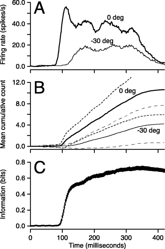
Time course of cumulative spike count and information for a representative MT neuron. A, Time course of average firing rate for two directions of stimulus motion. B, Time course of cumulative spike count for the same two directions. Continuous and dashed lines show mean and one SD. In A and B, the bold and fine lines show responses for motion in the preferred direction and 30° off preferred direction. C, Time course of mutual information about motion direction from cumulative spike count. The variable thickness of the line indicates the time course of the SD of information.

Two different ways of analyzing the data from our full sample of MT neurons show that information about direction almost always accumulates most rapidly early in the response, after just a few spikes have been fired. In Figure 4A, each symbol summarizes responses of an individual neuron and plots information 256 msec after response onset versus information 100 msec after response onset. Most neurons plot just above the line of slope 1, indicating that only slightly more information is available after counting spikes for 256 msec than after counting for only 100 msec. If we consider only the neurons with >0.2 bits of direction information, then on average 78% of the maximum amount of information obtainable from counting spikes for 256 msec is available 100 msec after response onset (range, 50–113%; n = 26). The rapid approach to maximum information does not represent a limit imposed by the stimulus entropy: information about direction in the discharge of MT neurons always was well below the 3.7 or 4.09 bits of direction information contained in the stimulus sets of 13 or 17 stimuli.

Figure 4.

Population summary of the time course of information from cumulative spike count. A, Information available 256 msec after response onset is plotted against that available at 100 msec. Each symbol shows measurements from one neuron, and the dashed line has unity slope. B, Each curve shows data from one MT neuron and plots information from cumulative spike count as a function of the cumulative spike count averaged across directions. Thus, time runs to the right along the x-axis as spike count increases. Information has been normalized for the maximum information provided by each neuron. Neurons were included (n = 27) if they provided > 0.2 bits of information about direction. The bold curve plots data from the example neuron shown in Figures 2 and 3.

Figure 4B replots the data from each of our neurons in a way that shows how information about direction accumulates as a function of the number of spikes the neuron has fired. To obtain the values on the x-axis, we averaged the responses across all directions of motion in the stimulus set and determined the average cumulative spike count at each time in 8 msec increments. The fractional values of average cumulative spike count on the abscissa should not be a concern: a value of 0.1 means that a single count was present in that bin for 1 of 10 trials, on average. To obtain the values on the y-axis, we computed direction information from the cumulative spike count at each 8 msec time step and normalized by the maximum value of information throughout the response. We then plotted normalized information as a function of average cumulative spike count for each 8 msec bin in our averages. For every neuron, direction information rose quickly, usually reaching or coming close to the maximum before three spikes had been fired, on average. In one-third of our sample (12 of 36), more than half of the maximum information was available once an average of one spike had been fired.

Coding capacity and efficiency of MT neurons

One of the features of Figure 4A is wide variability among neurons in the peak amount of information about direction. Some neurons can provide just over 1 bit of information out of the 3.7–4.1 bits in the stimulus set, whereas others provided only a fraction of a bit. The variability among MT neurons raises the question of whether all MT neurons have the same intrinsic capacity to transmit information and, if so, what fraction of that capacity is used for the stimulus set we provided as visual stimuli. To answer this question, we next compute the response entropy or coding capacity from the spike count for each MT neuron in our sample.

Figure 5 shows that the coding capacity of all cells in the population is near the theoretical maximum limit imposed by their average firing rate (Eq. 4). The thin lines in Figure 5 show the entropy of the spike count distribution (Eq. 3) for our sample of MT neurons as a function of the average number of spikes fired with time during the response. Despite substantial differences in the details of the neural responses among the different cells in our sample, the entropy as a function of mean count is almost the same for all neurons, and their capacities are quite close to the theoretical limit set by Equation 4 (bold line). The peak coding efficiencies for direction of motion, defined as the maximum information about direction divided by the response entropy, ranged from 3 to 40% in our sample (mean, 20%). Figure 5 also illustrates that the capacity to carry information grows sublinearly with the spike count, a factor that will make a minor contribution to the fact that MT neurons reach ∼80% of maximal information about direction within the first 100 msec of the neural response.

Figure 5.

Coding capacity (entropy) of neural responses in MT. The fine curves show the entropy of spike count distributions as a function of the average spike count across all directions for 36 MT. The bold line shows the maximum entropy as a function spike count (Eqs. 3, 4).

Possible reasons for the rapid saturation of information about direction of motion

The previous section shows that the failure to gain substantial additional information about motion direction after the first 100 msec of neural responses cannot be attributed to saturation at the maximum coding capacity of the MT neuron. We next show that it also cannot be attributed to a decrease in directional tuning as a function of time during stimulus motion or to special properties of the transient response shown by many MT neurons for the onset of motion.

We quantified direction tuning by computing the average spike count during the first and second 100 msec period after the onset of the response as a function of direction of motion and fitting the data from each time period with a Gaussian function. As shown in the two examples in Figure 6, B and C, the tuning bandwidth, quantified as 2σ from the Gaussian fits, did not change consistently as a function of time. For the cell in Figure 6 B, the bandwidth decreased by 3° and the preferred direction shifted by 15° in the second 100 msec after the onset of the response (gray curve) compared with the first 100 msec (black curve). For the cell in Figure 6C, the bandwidth increased by 23° and preferred direction did not shift. Figure 6 A summarizes the data from the full population by plotting tuning bandwidth in the second 100 msec interval after the onset of the neural response to motion versus that in the first 100 msec after the response onset. Some of the cells with broader tuning also showed different bandwidths at different times, but the data were nearly equally spaced around the line of slope 1, indicating that direction tuning was maintained throughout the response across our sample of neurons.

Figure 6.

Absence of change in tuning bandwidth with time during response. A, Tuning bandwidth in the first 100 msec of the response plotted as a function of bandwidth in the second 100 msec of the response. Each symbol summarizes data from one neuron of the 33 for which a tuning curve could be fitted. Three cells were omitted because they had atypical tuning bandwidths that were >400° or <20°. Bandwidth was defined as twice the SD of the Gaussian function that provided the best fit to the mean spike count as a function of stimulus direction. The dashed line has slope of 1, and the continuous line is the best linear fit through the population assuming equal variance in both ordinate and abscissa (type II linear regression): slope, 1.2 ± 0.2; intercept, –5 ± 19°. B, C, Mean firing rate is plotted as a function of stimulus direction for two units in our sample. Black and gray curves show Gaussian fits to the first and second 100 msec of the responses. The filled triangle and circle in A show measurements for the two neurons illustrated in B and C, respectively.

To test whether the early saturation of information is a consequence of the initial transient response of many MT neurons for the onset of motion, we compared the time course of information about direction when we started counting spikes before versus after the initial transient response. Figure 7A shows that information rose quickly and saturated whether we started counting spikes and computing information about direction from the onset of stimulus motion (black), at the beginning of the sustained component of the response (medium gray), or 52 msec later (light gray). In the example of Figure 7A, however, the maximum information from counting spikes did depend on when we started counting, indicating that the initial transient response may make a special contribution to information about the direction of motion. Figure 7D shows that the same feature of information time course was maintained across the population of cells we recorded. Whether we started counting spikes at the onset of stimulus motion (open circles), at the start of the sustained interval (open triangles), or 52 msec later (open squares), the points lie just above the line of slope 1, indicating that the information available 256 msec after the start of the neural response is only slightly greater than that available 100 msec after the start of the analysis window.

Figure 7.

Analysis of the time course of information for spike counts in different analysis intervals and bins. A, Time course of information about direction from cumulative spike count starting at different times: the black, dark gray, and light gray lines show the mean and SD of information when counting started from motion onset, the beginning of the sustained response, and 50 msec after the beginning of the sustained response. The symbols next to each curve indicate the shapes used to plot the population summaries in D. B, Time course of information from spike counts in 20 msec bins. C, Time course of information in non-overlapping 20 msec bins normalized for the number of spikes in each bin. In B and C, error bars show SDs. A–C show analyses from the same neuron. D, Information for 100 msec after the beginning of the counting window is plotted as a function of the information 256 msec after response onset. Each neuron is represented by three points: an open circle, open triangle, and filled circle for analyses that began at motion onset, the start of the sustained response, and 50 msec later. E, Population summary(n = 36) of information about direction from spike counts in 20 msec bins. Each point shows data from one neuron and plots peak information in the transient period versus the average information in the sustained period. F, Population summary of normalized information from spike counts in 20 msec bins. Each symbol shows data from one neuron and plots peak information per spike in the transient period versus the average information per spike in the sustained period. In E and F, filled circles and open squares show neurons with transient/sustained ratios of firing rate greater or less than 1.6. In D–F, the dashed line has a slope of 1.

Information about direction from spike counts in brief time bins

Until now, we examined the information about direction in cumulative spike counts. We next ask whether different parts of the neural response contribute differentially to the accumulation of a direction estimate in MT by computing information from spike counts in discrete time bins. When we counted spikes in non-overlapping 20 msec bins, the information about direction from the neuron shown in Figure 7B was greatest during the onset transient but settled to a sustained level that endured throughout the response to stimulus motion. The scatter plot in Figure 7E shows that this was true throughout our sample of MT neurons: information about direction was larger during the transient than the sustained response but remained steady throughout the sustained response. In 20 of 36 neurons, an individual 20 msec bin provided more than half of the total information available from counting spikes for 256 msec.

More information about direction might be encoded in time bins during the response onset transient because either there are more spikes in the transient or the spikes themselves are individually more informative. Figure 7C plots the time course of information in 20 msec bins, normalized by the average count in each bin over all directions, for the same MT neuron shown in Figure 7, A and B. The information per spike was slightly higher during the transient compared with the sustained period, indicating that the first spikes of the neural response were slightly more informative about motion direction. Across the population, the information per spike in the transient response was similar to that in the sustained period but was somewhat larger in many neurons (Fig. 7F). When evaluated in 20 msec bins for the 27 neurons that provided >0.2 bits of information about direction, the information transient/sustained ratio was significantly correlated to the firing rate transient/sustained ratio (r = 0.76; p < 10^–5), but the information per spike transient/sustained ratio was not. Furthermore, there was no correlation between the transient/sustained ratios for information and information per spike. The quantitative summary analysis in Table 1 shows that the mean transient sustained ratios for information per spike were >1, indicating that much but not all of the “extra” information available in small time windows near the start of the response can be attributed simply to the fact that these windows contain more spikes.

Table 1.

Analysis of effect of bin width on measures of information in the transient and sustained portions of MT neuron responses

Information from counts in time windows
Bin width (msec)	Peak information in transient period window across cells (bits)					Mean information in sustained period windows across cells (bits)					Information transient/sustained ratio
		Range	Mean	Median	Range	Mean	Median	n	Range	Mean	Median
4	0.01-0.34	0.10	0.09	0-0.19	0.04	0.03	27	0.4-10.8	3.5	2.7
8	0.02-0.58	0.19	0.18	0.01-0.34	0.08	0.06	27	0.8-8.6	3.0	2.5
16	0.03-0.79	0.30	0.26	0.02-0.56	0.15	0.12	27	0.6-8.1	2.7	2.1
20	0.04-0.83	0.34	0.28	0.02-0.62	0.18	0.14	27	0.5-7.5	2.6	2.3
32	0.06-0.94	0.42	0.37	0.03-0.74	0.24	0.22	27	0.6-6.5	2.3	2.0
64	0.11-0.96	0.46	0.43	0.06-0.88	0.35	0.36	27	0.4-4.4	1.6	1.3
Information per spike in time windows
Bin width (msec)	Peak information per spike in transient period across cells (n = 27) (bits/spike)					Mean information per spike in sustained period across cells (n = 27) (bits/spike)					Information per spike transient/sustained ratio
		Range	Mean	Median	Range	Mean	Median	n	Range	Mean	Median
4	0-1.54	0.67	0.64	0.06-1.09	0.44	0.43	26	1.0-6.5	2.1	1.6
8	0.04-1.44	0.66	0.70	0.06-1.04	0.44	0.43	27	0.7-4.8	1.7	1.5
16	0.06-1.27	0.57	0.58	0.04-0.94	0.42	0.41	27	0.6-4.9	1.6	1.4
20	0.03-1.15	0.53	0.53	0.04-0.92	0.41	0.39	27	0.5-5.0	1.5	1.3
32	0.04-1.01	0.43	0.46	0.03-0.80	0.36	0.39	27	0.4-2.7	1.3	1.2
64	0.02-0.89	0.33	0.32	0.02-0.59	0.28	0.29	27	0.2-1.9	1.2	1.2

The bin width chosen for analysis had an impact on the exact value of information we calculated, but changes in the bin width from 4 to 64 msec did not alter the general conclusion. The data in Figure 7 were analyzed using a bin width of 20 msec. As illustrated in Table 1, both the peak information and sustained information obtained by counting spikes increased as bin width increased from 4 to 64 msec, whereas the information per spike decreased. The information transient/sustained ratio, defined as the peak information during the first 100 msec of the response divided by the average information during the rest of the response, decreased as bin width increased for both the total information in bits and the information per spike. However, it remained statistically larger than one even for the largest bin widths of 64 msec.

Within-trial correlations in spike counts

In this section, we show that correlations in the fluctuation of spike counts across different time intervals within individual trials is one major reason why information fails to accrete substantially through counting for >100 msec. We show this feature of the data by (1) analysis of the relationship between the variance and the mean spike count in bins of different durations, (2) evaluation of the variation in spike count across and within trials, and (3) direct assessment of the correlations in spike count across time in individual trials.

First, we computed the Fano factor, defined as the variance of spike count divided by the mean spike count. If there are correlations in spike count across time within individual trials, then there would be more variation in spike count between trials than within trials and the Fano factor should increase as a function of the duration of the interval used to count spikes. Figure 8A plots the Fano factor as a function of time for a representative MT neuron, including responses for all directions of stimulus motion. The Fano factor measured in bins with widths of 20 msec (open circles) and 50 msec (filled triangles) remains close to unity throughout the time of stimulus motion, as would be expected if spikes were generated by an approximately Poisson process. However, the Fano factor of the cumulative spike count is greater than one and increases as the effective bin width is increased by counting longer into the trial (thin line).

Figure 8.

Time course of the variation of spike counts in MT neurons. A, Analysis of a representative neurons showing the Fano factor of spike count plotted as a function of time. Open circles, filled triangles, and the curve without symbols show data when spike counts were measured in 20 msec bins, 50 msec bins, and accumulated in 2 msec increments. The horizontal line indicates a Fano factor of 1, expected for a Poisson process. B, Fluctuating curve shows the total spike count in the full 768 msec of each trial plotted as a function of trial number within the experiment for all stimuli that presented motion in the preferred direction of the neuron. A and B show data from the same neuron. The solid and dashed horizontal lines indicate the mean total spike count across the experiment, plus and minus one SD. C, Correlations between spike counts in the first and second 128 msec of neural responses for a representative MT neuron. Each pixel in the graph is plotted at locations on the x-axis and y-axis that indicate the difference between the actual response and mean responses in the first and second 128 msec of the response. The value on the grayscale indicates the joint probability of measuring a given pair of fluctuations in spike count in individual responses to preferred direction motion. D, Summary of the analysis in A for our sample of MT neurons. Each curve shows the distribution of Fano factors across the sample. The bold curve, fine curve, and curve with small filled circles summarize data measured in bins of duration 10, 100, and 256 msec. E, Tail of the rate normalized, connected (shuffle-corrected) autocorrelation of spike count for a representative MT neuron responding to preferred direction motion. Filled symbols with error bars and symbol-less error bars show the autocorrelation functions for the actual spike counts and synthetic Poisson shuffled counts. Error bars represent SDs of correlation values computed from multiple random samples of half of the dataset. C and E show data from the same MT neuron. F, Summary of the average values of the autocorrelation over 50–150 msec lag. White bars and black bars show probability density distributions for actual data and synthetic Poisson shuffled data.

Accumulating the distributions of Fano factors across all MT neurons and all bins in our analysis shows that this effect holds across the population (Fig. 8D). For 10 msec time bins (heavy black line without symbols), the distribution of Fano factors is narrow and peaks at unity, with a significant fraction of sub-Poisson events. For 100 msec bins (thin gray curve) and the whole 256 msec response (solid curve with symbols), the distributions are broader and contain many examples in which the Fano factor was greater than unity. Thus, on average, the Fano factor grows with the size of the time window over which spike count statistics are computed, implying that there are correlations in the trial-by-trial fluctuations in spike count that span the duration of the response.

Second, we evaluated trial-to-trial changes in the responsiveness to a single stimulus. For example, Figure 8B plots the total spike count as a function of trial number for the responses of one neuron to stimulus motion in its preferred direction. Although the mean appears fairly stationary for the duration of the experiment, the total spike count for the entire 768 msec of individual trials fluctuated considerably from trial to trial: the mean spike count across the 180 trials was 11.1 spikes, and the SD was 4.9 spikes, yielding a Fano factor of 2.2. For the entire sample of MT neurons, the SD of the total spike count during 256 msec of target motion in the preferred direction ranged from 1.5 to 22.5 spikes, with a mean value of 5.4 spikes. The Fano factor ranged from 0.8 to 10.4 (mean of 3.6).

As an additional test of whether fluctuations in spike counts within different portions of the response were correlated across time, we analyzed the first and second 128 msec of each response separately. In each half of each trial, we computed the difference between actual spike count and the mean count across all trials in the time window. We then made plots like that in Figure 8C, in which the level of gray indicates the number of observations of each joint deviation of count from the mean in the first and second halves of the response. If the intensity of the grays is greatest near the line of slope 1, as in Figure 9C, then there is a correlation across time. The correlation means that a neuron tends to fire more (fewer) spikes in the second half of the response if it also fires more (fewer) spikes than average in the first half of the response. Deviations in the count from the mean were modestly but significantly correlated in the two time windows across our sample (p < 10^–7, comparing correlation coefficients from shuffled versus actual data). For the neuron used to create Figure 8C, the linear correlation coefficient for preferred direction motion was 0.51, close to the sample mean of 0.4 and similar to results found in MT neurons of awake monkeys by Uka and DeAngelis (2003). The magnitude of the correlation coefficient did not vary strongly as a function of direction within 60° of the preferred direction.

Figure 9.

Effect of removing temporal correlations on the time course of information about direction. A, Plots of information as a function of time for a representative neuron. The gray and black curves show the mean and SDs of information about direction for the actual cumulative spike count and from shuffled data. Vertical dashed lines mark the time window used to obtain the data plotted in B. B, C, Summary of the effect of shuffling the spike counts across the population. In B, each symbol shows data from one neuron and plots the increase in information between 56 and 256 msec after response onset for the shuffled data versus that for the actual spike counts. In C, each neuron is represented by two symbols plotting information measured 256 msec after response onset as a function of that measured 100 msec after response onset. Open and filled circles show results of analyses based on the actual and shuffled data. In B and C, the dashed lines have a slope of unity.

Third, we analyzed the time scale of temporal correlations in firing rate by computing the connected (shuffle-corrected) autocorrelation function (see Materials and Methods) for the responses of each neuron to stimulus motion for each stimulus direction. For the neuron responding to preferred direction motion illustrated in Figure 8E, the autocorrelation of the actual spike trains showed significant correlations out to >200 msec (bars with symbols). The synthetic Poisson autocorrelation, shown by the bars without symbols in Figure 8E, was not statistically different from zero across the analysis window. For our sample of MT neurons, the normalized, connected (shuffle-corrected) correlation functions had values that were broadly distributed between 0.6 and 21 spikes/sec at 100 msec lag (Fig. 8F, gray bars), with a mean of 6.2 spikes/sec. The tight grouping around zero at the same time lag for the synthetic Poisson data (Fig. 8F, black bars) indicates that such correlations cannot arise at random in a data set of this size. If we express the connected autocorrelation at 100 msec lag as a fraction of the time-averaged firing rate in the preferred direction, our sample ranged from 2 to 100%, with a mean of 24% and a median of 16%. The connected autocorrelation functions were fit well with an exponential function:

(9)

where the values of the parameters were as follows: time constant (τ) of 47–909 msec, mean of 162 msec; B, 0.7–56 spikes/sec, mean of 16 spikes/sec; A, –2.7 to +3.3 spikes/sec, mean of –0.3 spikes/sec. Note that the data in Figure 8F were based on analysis of responses for all directions of stimulus motion.

Information about direction in spike trains with temporal correlations removed

Figure 9 verifies the expectation that removing the correlation within trials allows information about direction to accumulate throughout the duration of the stimulus. For each neuron, the data for each direction of target motion was shuffled independently in each time bin according to the strategy outlined in Materials and Methods, generating a synthetic Poisson analog of the original spike train. The time course of information about direction from the cumulative spike count in these data are shown for one neuron in Figure 9A, illustrating a steady rise of information throughout the stimulus for the synthetic Poisson data (black) compared with the actual data (gray). In the shuffled data, only 64% of the final value of information is available 100 msec after the onset of the response, whereas 84% was available in the actual data.

We summarized the effects of temporal decorrelation on the accumulation of information over time in two ways. First, for each neuron, we measured how much information is accumulated in the 200 msec interval between 56 and 256 msec after response onset for the actual and the synthetic Poisson data. When the information accumulated from the decorrelated spike trains is plotted as a function of that from the real data (Fig. 9B), almost all of the neurons plot above the line of slope 1, indicating that removing the within-trial correlations in firing rate allows a larger accumulation of information during the sustained part of the response. Second, we repeated the graph of Figure 4B for the synthetic Poisson data. Figure 9C plots information 256 msec after the onset of the response as a function of information 100 msec after response onset, with each MT neuron represented by two data points. The information measured from the shuffled data (filled symbols) plotted above that from the actual data (open circles), indicating a greater accumulation of information during the sustained period in the decorrelated data than in the actual data.

Direction discrimination by MT neurons

In most of the paper, we evaluated the temporal accumulation of information about direction and the reasons information saturates early in the response. We now turn to the question of how well, rather than how quickly, MT neurons can discriminate different directions of target motion.

To determine the effective directional discrimination threshold of MT neurons, we computed the information, or equivalent percentage correct, for pairs of directional stimuli. Inspection of tuning curves like that in Figure 2C supports the intuitive expectation that any given MT neuron will discriminate directions that fall on the steep flanks of its tuning curve better than directions that straddle its peak, as found with frequency discrimination in the auditory system (Siebert, 1968). To quantify this intuition, we computed the information about direction for each pair of stimulus directions, I(θ₁,θ₂), from the cumulative spike count binned at 2 msec resolution. For each neuron, we constructed graphs like those in Figure 10A, which plot the information computed from each pair of directions as a function of their directional separation, θ₁ – θ₂, and mean direction, (θ₁ + θ₂)/2. For example, 30° and 45° form a pair with a 15° directional separation and a mean direction of 37.5°, whereas –7.5° and +7.5° form a 15° pair with a mean direction of 0°. To facilitate evaluation of discrimination of directions at different places on the direction tuning curves, we connected the points with the same separation between directions and plotted the data as a function of the mean direction of the pair.

Figure 10.

Discriminability of pairs of motion directions based on the first 100 msec of responses of MT neurons. A, Analysis for an individual neuron. Each point plots the information about direction computed from responses to a pair of stimuli of a mean direction specified by the y-axis and a directional separation specified by the symbol. Points have been connected into curves if they had the same directional separation. Numbers to the left of each curve indicate the directional separation in degrees. The left-hand y-axis plots information in bits, and the right-hand y-axis plots the equivalent percentage of correct choices based on the responses of the neuron. The horizontal dashed line marks a threshold for discriminability defined as 69% correct or 0.107 bits of information. B, Summary of the ability to discriminate pairs of motion directions for the population of MT neurons. Each pixel summarizes the population data for pairs of stimulus directions of directional separation and mean direction given by the location of the pixel on the y-axis and x-axis, respectively. Colors indicate the percentage of the MT sample (n = 36) for which direction discrimination was above the 69% correct threshold after 100 msec of neural response. In both A and B, a mean direction of zero means that the two stimulus directions were equally spaced on opposite sides of the preferred direction.

For each set of connected points, information is smallest when the mean direction is zero because the pair straddles the preferred direction and the means and variances of the responses are similar for each direction in the pair. Information increases as the mean direction becomes positive or negative, because the pair straddles a direction on the flank of the tuning curve and the distributions of the responses to the two directions are more separated. Information decreases again as the mean direction of the pair of stimuli gets too large, because the neural responses decrease and eventually are zero when the mean direction is far from the preferred direction. Comparison of the different curves in Figure 10A reveals that information increases at any given mean direction as the directional separation increases. Nearly all MT neurons (33 of 36) had the largest values of information, and therefore discriminated direction best, when the mean direction of the pair of stimuli fell on the flanks of their tuning curves. The other three neurons were not able to discriminate any pair of directions. The analysis in Figure 10A is for the first 100 msec of the neural response. Nearly identical results were obtained (but not shown) for the full 256 msec of the neural response. Averaged across pairs and mean directions, pairwise direction information 256 msec after response onset is only 0.1 bit larger than 100 msec after response onset.

We used an approach outlined in Materials and Methods to relate the values of information plotted in Figure 10 to an equivalent percentage correct for a discrimination task. We defined threshold discriminability (Fig. 10A, horizontal dashed line) as the value of information that corresponds to 69% correct, equivalent to a signal-to-noise ratio of 1 in the model problem of detecting a signal against a background of Gaussian noise (Green and Swets, 1966). Using this threshold, the responses of the neuron shown in Figure 10 are sufficient to discriminate a 30° difference in stimulus directions at most points on the tuning curve and a 15° difference at a few. For the 34 of 36 cells of our sample that could discriminate at least one pair of stimuli, direction discrimination thresholds ranged from 7.5° to 75°, with a mean of 27° after 100 msec of response; the mean fell to 21° after the full 256 msec of response.

To summarize the ability of our full sample of MT neurons to discriminate directions, we first corrected for the fact that 24 MT neurons were recorded with 15° directional spacing (13 directions), whereas 12 neurons had some stimuli separated by only 7.5° (17 directions). For all neurons, we interpolated the information values for each curve in Figure 10A along the mean direction axis from –60° to +60° in 7.5° steps, as if each neuron had been sampled with the same directional spacing of 7.5°. Figure 10B uses a color value in each entry in the graph to show the fraction of MT neurons in our sample that could discriminate a pair of stimuli with given directional means (x-axis) and separations (y-axis) at a level of 69% correct (I > 0.107 bits). The red and yellow pixels in the top left and right corners of the image show that a large fraction of the sample was able to discriminate two stimuli with large directional separations and mean directions on the flank of the direction tuning curve. The blue columns down the middle of the image show that few neurons were able to discriminate even large directional separations when they straddled the peak of the direction tuning curve. The dark blue row along the bottom of the image shows that some, but only very few, neurons were able to discriminate directional separations of 7.5° when the mean direction was on the flank of the direction tuning curve.

Thirty-one percent of our sample (11 of 36) could discriminate –30° from –45° stimulus motion (mean direction, –37.5°; difference, 15°), whereas only 3% (1 of 36) could discriminate motions that also differed by 15° but were 7.5° on either side of the preferred direction (mean direction, 0°; difference, 15°). The average threshold within 60° of the preferred direction ranged from 16° to 75° across the sample (mean of 37°) after 100 msec of response; the sample mean fell only slightly to 35° after the full 256 msec of response. We doubt that the poor discrimination of direction by individual MT neurons is an artifact of our analysis, because we used a computation that overestimates the percentage correct and a low threshold of 69% correct for categorizing a pair of stimuli as discriminable.

Discussion

One of the most important intuitions about the connection of neural responses to perception and behavior is that averaging suppresses noise. To make reliable decisions and to provide accurate commands for motor behavior in the face of noise, the nervous system accumulates evidence over time (Britten et al., 1992, 1996; Gold and Shadlen, 2003) and across large populations of neurons (Georgopoulos et al., 1986; Lee et al., 1988; Treue et al., 2000). The observations of Zohary et al. (1994) on correlations among the responses of neurons in MT established that simple ideas about the improvement of precision with averaging are not correct and led a number of groups to reexamine the problem of noise reduction by accumulating evidence across populations of neurons (Abbott and Dayan, 1999; Panzeri et al., 1999; Bair et al., 2001). Our results can be viewed as an extension of this discussion to the problem of averaging across time.

Challenges of averaging over time

In some systems, averaging over time cannot produce more precise representations of ongoing sensory stimuli simply because the relevant neurons respond transiently. Even cells in visual cortex that generate maintained responses often have a substantial transient component to their response at stimulus onset, and a number of experiments indicate that these transients make a disproportionate contribution to the sensory discrimination power of the neuron (Oram and Perrett, 1992; Tovee et al., 1993; Heller et al., 1995; Muller et al., 2001). The transient/sustained responses of MT neurons (Lisberger and Movshon, 1999) to moving visual stimuli provide an excellent opportunity to analyze averaging over time in detail.

In MT neurons, spike counts provide information about motion direction that saturates quickly after the onset of the response, as if this information were dominated by the initial transient. Our analysis of the data, however, indicates that the saturation of information in MT cannot be ascribed solely to the transient behavior of the neural responses. Information about motion direction saturates with time even if we start counting spikes after the transient response is over. We conclude that information saturates quickly because integration over times in excess of 100 msec fails to produce the expected suppression of noise in the response, not because the first few spikes after stimulus onset are inherently much more informative.

The failure to suppress noise by averaging over time can be traced to correlations within the spike train of single neurons, much as correlations among the spike counts of different neurons can limit the suppression of noise by averaging over a population (Zohary et al., 1994). Even when we corrected for time variation in firing rates, the spike trains of MT neurons in our population exhibited correlations that lasted for 100 msec or more. The failure to reduce the variance by averaging over time is exactly what is measured by the Fano factor, the ratio of variance to mean spike count. In our data, Fano factors were small when measured in small time windows but increased several-fold when we accumulated spike counts in a larger time window. If the Fano factor were to grow exactly in proportion to the integration time, it would mean that the correlations in the spike train were so strong that averaging a sustained response over time would yield zero improvement of signal-to-noise ratio. MT neurons are not quite in this limit. Hence, there is some increase of information as a function of integration time but much less than expected in the absence of correlations.

The long-lasting correlations that we observe in the spike trains of MT neurons have analogs in other systems; in particular, Teich et al. (1996) have drawn attention to the growth of Fano factors with integration time in many different classes of sensory neurons. For many tasks that depend on visual signals emanating from MT, discrimination performance improves with stimulus duration T, but the improvement is much slower for long durations than the dependence expected if the system were integrating the responses of neurons without long-term correlations in their spike trains (Britten et al., 1992; Gold and Shadlen, 2003; Uka and DeAngelis, 2003). From a theoretical point of view, it is possible that these behavioral observations are connected to our neural data: if neural Fano factors grow as T^b, where the exponent b describes the degree of temporal correlation, and discrimination is based on integration of spike counts, then discrimination thresholds will improve as 1/T^{(1 – b)/2}. Growth of Fano factors with integration time, as we observed, should contribute to a reduced ability for perceptual discriminations to improve with stimulus duration.

Behavioral correlates of rapid saturation of information

The converse of the slow improvement of discrimination threshold with time discussed above is that fine perceptual discriminations and accurate motor behavior often are possible even with very brief stimuli. Thorpe et al. (1996) have drawn attention to the fact that surprisingly sophisticated perceptual decisions can be made very rapidly, and de Bruyn and Orban (1988) have shown that human direction discrimination saturates with stimulus presentations lasting <100 msec. Of particular relevance is the motivation for the experiments discussed here: MT neurons provide the input for smooth pursuit eye movements (Newsome et al., 1985; Groh et al., 1997; Born et al., 2000), which are initiated with appropriate speeds and directions based on 100 msec of target motion (Lisberger and Westbrook, 1985). Preliminary experiments indicate that even the earliest components of pursuit motor output are highly direction specific (Osborne et al., 2003). Thus, the rapid accumulation of information that we observe for single neurons in MT is matched to the time scale on which information about target direction is used to initiate pursuit. On the basis of the fact that counting spikes for just 20 msec provides more than half of the information that one can gain by counting spikes for 256 msec, we would predict that many behaviors would be precise even with very short presentations of motion.

Although information about direction is available very quickly, there is a discrepancy between the amount of information provided by single neurons and the precision of behavioral responses. Smooth pursuit eye movements have an accuracy that corresponds to discrimination thresholds of a few degrees on a time scale of 100 msec (Osborne et al., 2003), equivalent to >4 bits of information about direction. In contrast, most MT neurons in our sample could not make reliable discriminations with better than 15° accuracy, and none of the cells provided >1.5 bits of information about direction on the basis of spike counts. Although it is possible that additional information is present in the precise timing of the first few spikes in the response of an MT neuron, this possibility did not yield to standard approaches for our data set. Therefore, it is almost certainly essential to combine signals across the population of MT neurons to reach the behavioral performance of pursuit. Indeed, given the small increment in information achievable by averaging across time, averaging across the population of MT neurons seems like a better strategy. We do not think that this conclusion is undermined by our choice to record from MT neurons in anesthetized monkeys, which was dictated by the need to record from neurons for a long time to obtain enough repetitions of each stimulus. Indeed, the agreement between our numbers for the correlations across time in anesthetized monkeys and those of Uka and DeAngelis (2003) in awake monkeys underscores the validity of our data for comparison with pursuit behavior.

In apparent contrast to our results, previous work on the reliability of MT responses has emphasized the similarity of behavioral and neural thresholds for discrimination of the direction of motion for stimuli consisting of low-correlated motion signals embedded in large amounts of directional noise (Britten et al., 1992). However, when viewed on the 100–200 msec time scale considered here, the discrimination power of MT neurons for the stimuli with directional noise is quite poor and typically worse than the reported behavioral performance on these time scales (cf. Britten et al., 1992, their Fig. 11) (see also Uka and DeAngelis, 2003).

It is important to remember that the information measures we find here, like all quantitative characteristics of neural responses, depend on the ensemble of stimuli used in the experiment. Our choice of stimuli was motivated by the connection to behavioral experiments on smooth pursuit, so that we would be comparing responses to identical stimuli when we compare the information content of neural and behavioral responses. Thus, we chose target motions that match those used to analyze pursuit behavior in the laboratory and that fall within the natural stimulus set for pursuit, if not for all visual tasks. We chose not to vary other visual parameters such as luminance or contrast, although we doubt that would change the basic observation that information about direction saturates early in the response. Under very different stimulus conditions, in which motion trajectories vary dynamically in time, neurons can provide information about the stimulus at constant rates (rather than saturating), but this is possible only because different temporal windows in the response provide information about velocity at different moments in time (Bialek et al., 1991; Buracas et al., 1998); simple integration of the spikes over time is of limited effectiveness in this case because of the dynamics of the stimulus itself.

Under our stimulus conditions, the time scale for saturation of information corresponds to counting rather few spikes. In almost all neurons, information saturated before an average of three spikes had been fired, and, in one-third of the population, the half-saturation point had been passed once one spike (on average) had been fired. Because this time scale also corresponds to the initiation of pursuit, the contribution of each cell to the population code that drives pursuit must be conveyed by the arrival times of just these few spikes.

References

- Abbott LF, Dayan P (1999) The effect of correlated variability on the accuracy of a population code. Neural Comput 2: 91–101. [DOI] [PubMed] [Google Scholar]
- Abbott LF, Rolls ET, Tovee MJ (1996) Representational capacity of face coding in monkeys. Cereb Cortex 6: 498–505. [DOI] [PubMed] [Google Scholar]
- Allman J, Miezin F, McGuiness E (1985) Direction- and velocity-specific responses from beyond the classical receptive field in the middle temporal visual area (MT). Perception 14: 105–126. [DOI] [PubMed] [Google Scholar]
- Bair W, Zohary E, Newsome WT (2001) Correlated firing in macaque visual area MT: time scales and the relationship to behavior. J Neurosci 21: 1676–1697. [DOI] [PMC free article] [PubMed] [Google Scholar]
- Bialek W, Rieke F, de Ruyter van Steveninck RR, Warland D (1991) Reading a Neural Code. Science 252: 1854–1857. [DOI] [PubMed] [Google Scholar]
- Born RT, Groh JM, Zhao R, Lukasewycz SJ (2000) Segregation of object and background motion in visual area MT: effects of microstimulation on eye movements. Neuron 26: 725–734. [DOI] [PubMed] [Google Scholar]
- Britten KH, Shadlen MN, Newsome WT, Movshon JA (1992) The analysis of visual motion: a comparison of neuronal and psychophysical performance. J Neurosci 12: 4745–4755. [DOI] [PMC free article] [PubMed] [Google Scholar]
- Britten KH, Newsome WT, Shadlen MN, Celebrini S, Movshon JA (1996) A relationship between behavioral choice and the visual response of neurons in macaque MT. Vis Neurosci 13: 87–100. [DOI] [PubMed] [Google Scholar]
- Buracas GT, Zador AM, DeWeese MR, Albright TD (1998) Efficient discrimination of temporal patterns by motion-sensitive neurons in primate visual cortex. Neuron 20: 959–969. [DOI] [PubMed] [Google Scholar]
- Cook EP, Maunsell JHR (2002) Dynamics of neuronal responses in macaque MT and VIP during motion detection. Nat Neurosci 5: 985–994. [DOI] [PubMed] [Google Scholar]
- de Bruyn B, Orban GA (1988) Human velocity and direction discrimination measured with random dot patterns. Vision Res 28: 1323–1335. [DOI] [PubMed] [Google Scholar]
- de Ruyter van Steveninck R, Bialek W (1988) Real-time performance of a movement sensitive neuron in the blowfly visual system: coding and information transfer in short spike sequences. Proc R Soc Lond B Biol Sci 234: 379–414. [Google Scholar]
- Distler C, Mustari MJ, Hoffman KP (2002) Cortical projections to the nucleus of the optic tract and dorsal terminal nucleus and to the dorsolateral pontine nucleus in macaques: a dual retrograde tracing study. J Comp Neurol 444: 144–158. [DOI] [PubMed] [Google Scholar]
- Georgopoulos AP, Schwartz AB, Kettner RE (1986) Neuronal population coding of movement direction. Science 233: 1416–1419. [DOI] [PubMed] [Google Scholar]
- Giolli RA, Gregory KM, Suzuki DA, Blanks RH, Lui F, Betelak KF (2001) Cortical and subcortical afferents to the nucleus reticularis tegmenti pontis and basal pontine nuclei in the macaque monkey. Vis Neurosci 18: 725–740. [DOI] [PubMed] [Google Scholar]
- Gold JI, Shadlen MN (2003) The influence of behavioral context on the representation of a perceptual decision in developing oculomotor commands. J Neurosci 23: 632–651. [DOI] [PMC free article] [PubMed] [Google Scholar]
- Green DM, Swets JA (1966) Signal detection theory and psychophysics. New York: Wiley.
- Groh JM, Born RT, Newsome WT (1997) How is a sensory map read out? Effects of microstimulation in visual area MT on saccades and smooth pursuit eye movements. J Neurosci 17: 4312–4330. [DOI] [PMC free article] [PubMed] [Google Scholar]
- Heller J, Hertz JA, Kjaer TW, Richmond BJ (1995) Information flow and temporal coding in primate pattern vision. J Comput Neurosci 2: 175–193. [DOI] [PubMed] [Google Scholar]
- Land MF, Collett TS (1974) Chasing behavior of houseflies (Fannia canincularis). A description and analysis. J Comp Physiol 89: 331–357. [Google Scholar]
- Lee C, Rohrer WH, Sparks DL (1988) Population coding of saccadic eye movements by neurons in the superior colliculus. Nature 332: 357–360. [DOI] [PubMed] [Google Scholar]
- Lisberger SG, Movshon JA (1999) Visual motion analysis for pursuit eye movements in area MT in macaque monkeys. J Neurosci 19: 2224–2246. [DOI] [PMC free article] [PubMed] [Google Scholar]
- Lisberger SG, Westbrook LE (1985) Properties of visual inputs that initiate horizontal smooth pursuit eye movements in monkeys. J Neurosci 5: 1662–1673. [DOI] [PMC free article] [PubMed] [Google Scholar]
- Maunsell JH, van Essen DC (1983) Functional properties of neurons in middle temporal visual area of the macaque monkey. I. Selectivity for stimulus direction, speed, and orientation. J Neurophysiol 49: 1127–1147. [DOI] [PubMed] [Google Scholar]
- Merrill EG, Ainsworth A (1972) Glass-coated platinum-plated tungsten microelectrode. Med Biol Eng 10: 495–504. [DOI] [PubMed] [Google Scholar]
- Muller JR, Metha AB, Krauskopf J, Lennie P (2001) Information conveyed by onset transients in responses of striate cortical neurons. J Neurosci 21: 6978–6990. [DOI] [PMC free article] [PubMed] [Google Scholar]
- Newsome WT, Wurtz RH, Dursteler MR, Mikami A (1985) Deficits in visual motion processing following ibotenic acid lesions of the middle temporal visual area of the macaque monkey. J Neurosci 5: 825–840. [DOI] [PMC free article] [PubMed] [Google Scholar]
- Osborne LC, Bialek W, Lisberger SG (2003) Tight correlation between sensory and motor estimates of target direction in primate smooth pursuit eye movements. Soc Neurosci Abstr 29: 603.17. [Google Scholar]
- Oram MW, Perrett DI (1992) Time course of neural responses discriminating different views of the face and head. J Neurophysiol 68: 70–84. [DOI] [PubMed] [Google Scholar]
- Oram MW, Foldiak P, Perrett DI, Sengpiel F (1998) The “ideal homunculus”: decoding neural population signals. Trends Neurosci 21: 259–265. [DOI] [PubMed] [Google Scholar]
- Palanca BJA, DeAngelis GC (2003) Macaque middle temporal neurons signal depth in the absence of motion. J Neurosci 23: 7647–7658. [DOI] [PMC free article] [PubMed] [Google Scholar]
- Panzeri S, Treves A (1996) Analytical estimates of limited sampling biases in different information measures. Network Comput Neural Syst 7: 87–107. [DOI] [PubMed] [Google Scholar]
- Panzeri S, Treves A, Schultz SR, Rolls ET (1999) On decoding the responses of a population of neurons from short time windows. Neural Comput 11: 1553–1577. [DOI] [PubMed] [Google Scholar]
- Pouget A, Dayan P, Zemel R (2000) Information processing with population codes. Nat Rev Neurosci 1: 125–132. [DOI] [PubMed] [Google Scholar]
- Priebe NJ, Lisberger SG (2002) Constraints on the source of short-term motion adaptation in macaque area MT. II. Tuning of neural circuit mechanisms. J Neurophysiol 88: 370–382. [DOI] [PMC free article] [PubMed] [Google Scholar]
- Priebe NJ, Churchland MM, Lisberger SG (2002) Constraints on the source of short-term motion adaptation in macaque area MT. I. The role of input and intrinsic mechanisms. J Neurophysiol 88: 354–369. [DOI] [PMC free article] [PubMed] [Google Scholar]
- Priebe NJ, Cassanello CR, Lisberger SG (2003) The neural representation of speed in macaque area MT/V5. J Neurosci 23: 5650–5661. [DOI] [PMC free article] [PubMed] [Google Scholar]
- Raiguel SE, Xiao D-K, Marcar VL, Orban GA (1999) Response latency of macaque area MT/V5 neurons and its relationship to stimulus parameters. J Neurophysiol 82: 1944–1956. [DOI] [PubMed] [Google Scholar]
- Rieke F, Warland D, de Ruyter van Steveninck R, Bialek W (1997) Spikes: exploring the neural code. Cambridge, MA: MIT.
- Roitman JD, Shadlen MN (2002) Response of neurons in the lateral interparietal area during a combined visual discrimination reaction time task. J Neurosci 22: 9475–9489. [DOI] [PMC free article] [PubMed] [Google Scholar]
- Salinas E, Abbott LF (1994) Vector reconstruction from firing rates. J Comput Neurosci 1: 89–107. [DOI] [PubMed] [Google Scholar]
- Shadlen MN, Britten KH, Newsome WT, Movshon JA (1996) A computational analysis of the relationship between neuronal and behavioral responses to visual motion. J Neurosci 16: 1486–1510. [DOI] [PMC free article] [PubMed] [Google Scholar]
- Shannon CE, Weaver W (1949) A mathematical theory of communication. In: The mathematical theory of communication. Urbana, IL: University of Illinois.
- Siebert WM (1968) Stimulus transformations in the peripheral auditory system. In: Recognizing patterns (Kollers PA, Eden M, eds), pp 104–133. Cambridge, MA: MIT.
- Snowden RJ, Braddick OJ (1991) The temporal integration and resolution of velocity signals. Vision Res 31: 907–914. [DOI] [PubMed] [Google Scholar]
- Strong SP, Koberle R, de Ruyter van Steveninck RR, Bialek W (1998) Entropy and information in neural spike trains. Phys Rev Lett 80: 197–200. [Google Scholar]
- Teich MC, Turcott RG, Siegel RM (1996) Temporal correlation in cat striatecortex neural spike trains. IEEE Eng Med Biol Mag Sept/Oct: 79–87.
- Thorpe S, Fize F, Marlot C (1996) Speed of processing in the human visual system. Nature 381: 520–522. [DOI] [PubMed] [Google Scholar]
- Tovee MJ, Rolls ET, Treves A, Bellis RP (1993) Information encoding and the responses of single neurons in the primate temporal visual cortex. J Neurophysiol 70: 640–654. [DOI] [PubMed] [Google Scholar]
- Treue S, Hol K, Rauber HJ (2000) Seeing multiple directions of motion-physiology and psychophysics. Nat Neurosci 3: 270–276. [DOI] [PubMed] [Google Scholar]
- Uka T, DeAngelis GC (2003) Contribution of middle temporal area to coarse depth discrimination: comparison of neuronal and psychophysical sensitivity. J Neurosci 23: 3515–3530. [DOI] [PMC free article] [PubMed] [Google Scholar]
- Watamaniuk SNJ, Sekuller R, Williams DW (1989) Direction perception in complex dynamic displays: the integration of direction information. Vision Res 29: 47–59. [DOI] [PubMed] [Google Scholar]
- Zohary E, Shadlen MN, Newsome WT (1994) Correlated discharge rate and its implications for psychophysical performance. Nature 370: 140–143. [DOI] [PubMed] [Google Scholar]