Classification and 3D averaging with missing wedge correction in biological electron tomography

Abstract

Strategies for the determination of 3D structures of biological macromolecules using electron crystallography and single-particle electron microscopy utilize powerful tools for the averaging of information obtained from 2D projection images of structurally homogeneous specimens. In contrast, electron tomographic approaches have often been used to study the 3D structures of heterogeneous, one-of-a-kind objects such as whole cells where image-averaging strategies are not applicable. Complex entities such as cells and viruses, nevertheless, contain multiple copies of numerous macromolecules that can individually be subjected to 3D averaging. Here we present a complete framework for alignment, classification, and averaging of volumes derived by electron tomography that is computationally efficient and effectively accounts for the missing wedge that is inherent to limited-angle electron tomography. Modeling the missing data as a multiplying mask in reciprocal space we show that the effect of the missing wedge can be accounted for seamlessly in all alignment and classification operations. We solve the alignment problem using the convolution theorem in harmonic analysis, thus eliminating the need for approaches that require exhaustive angular search, and adopt an iterative approach to alignment and classification that does not require the use of external references. We demonstrate that our method can be successfully applied for 3D classification and averaging of phantom volumes as well as experimentally obtained tomograms of GroEL where the outcomes of the analysis can be quantitatively compared against the expected results.

1. Introduction

The use of image-averaging strategies for the derivation of the three-dimensional structures of complex macromolecular assemblies is a central idea in low-dose biological electron microscopic analyses utilizing single-particle reconstruction approaches. These methods rely in general on the premise that differences observed among projection images of different copies of the same object arise from differences in the orientation of the object relative to the electron beam. These assumptions are not applicable when macromolecular assemblies are present in the context of larger entities such as cells and viruses, where projection images include contributions from the entire specimen. Electron tomography can be used to obtain 3D representations of each of these larger, complex, one-of-a-kind entities. The reconstructed volumes contain multiple copies of numerous macromolecules that can individually be subjected to 3D averaging. The development of methods to achieve this type of in situ 3D averaging is a topic of considerable interest at the interface between cell and structural biology because it allows image-averaging approaches to be combined with cryo-electron tomography to derive structural information on protein complexes present in near-native physiological environment.

In single-particle analysis of homogeneous molecular complexes, two-dimensional images corresponding to projections in arbitrary orientations are classified in order to find out which images correspond to similar views so that they can be aligned and averaged allowing the generation of three-dimensional models. If images in the collection are generated from different three-dimensional conformations, a second level of classification is required for identifying corresponding views so that each conformation can be reconstructed separately. In principle, given a collection of 3D tomographic images representing noisy copies of different conformational states, we can use the same rationale as before to identify subsets of images corresponding to distinct conformations so they can be separately aligned and averaged in three dimensions. In light of this analogy, many of the general procedures developed for single-particle microscopy can be readily adapted for tomographic averaging even though some fundamental differences exist between the two. For example, each image processing step is now more computationally demanding because of the added dimension (this is specially true for alignment routines in three dimensions). Also the signal-to-noise ratios are comparably lower because the total electron dose is usually fractionated over the entire tilt series. Equally important is the fact that tomographic reconstructions are affected by a missing wedge of information in reciprocal space that requires specialized processing routines that compensate for this effect. One advantage however, is that the contrast is higher than it would be for a projection through the same thickness of material and this increase in contrast may positively impact the ability to identify heterogeneity in the reconstructed sub-volumes.

To address these problems, we present here a comprehensive framework for the alignment, classification, and averaging of tomographic volumes that is computationally efficient, explicitly accounts for the missing wedge, and does not require external references or any enforcement of symmetry even in the case of symmetric macromolecules.¹ Modeling the missing wedge as an occluding mask in reciprocal space, we align two volumes by minimizing their “dissimilarity score”, only measured over regions where both volumes have no missing information. The best rotational transformation relating the two volumes is computed rapidly using the convolution theorem within the Spherical Harmonics framework, avoiding the use of exhaustive angular search while at the same time accounting for the missing wedge. Classification of volumes is also done exclusively using overlapping information in reciprocal space, eliminating the bias caused by the presence of the missing wedge. Finally, we adopt an iterative approach to alignment and classification that progressively improves alignment parameters and gradually refines class averages representing the different conformations present in the data. Our iterative procedure does not require the use of external references for initialization which can strongly bias the results. Further, we make no assumptions about the presence of symmetry at any stage of the procedure, making this a general purpose tool for variability analysis of heterogenous sets of noisy volumes affected by the missing wedge. We present validation experiments using both synthetic and real experimental data to assess the performance and applicability of our approach.

The paper is organized as follows. In Section 2 we review previous work in single-particle analysis and electron tomography in the context of image alignment and classification. In Section 3 we introduce a metric for measuring dissimilarity between volumes affected by a missing wedge. The corresponding three-dimensional alignment problem is presented in Section 4 together with a novel computational method to find its solution. In Section 5 we present the classification strategy for variability analysis and in Section 6 we combine the alignment and classification routines into a single iterative refinement procedure. Validation experiments on both synthetic and real data are presented in Section 7 and a final discussion is given in Section 8.

2. Background

Successful averaging requires proper identification of homogeneous subsets of images (classification) and their subsequent combination in-phase (alignment) in order to effectively increase the signal-to-noise ratio. In single-particle microscopy, alignment and classification techniques represent distinct processing steps and are intrinsically different from those needed in tomography. However, the greatest similarity between processing in single particle and tomographic approaches is in the integral connection between alignment and classification steps which needs to be done concurrently in order to resolve contributions from different components in a heterogeneous population. We begin with a brief review of the previous literature on alignment and classification routines for tomography followed by a discussion of iterative alignment-classification strategies used in single-particle microscopy that are relevant to our work.

2.1. Sub-volume alignment in tomography

Alignment or registration techniques in three dimensions have been extensively studied in image processing including cross-correlation based approaches such as those used in analysis of electron microscopic images. These techniques however, are not directly applicable for aligning tomographic data because the missing wedge in reciprocal space is known to bias the result tending to align areas of missing information to one another. Previous studies have acknowledged this problem and various solutions have been proposed but a rigorous analysis has not yet been reported. Alignment of volumes affected by the missing wedge to an external reference that has no missing information (i.e., it is not altered by the presence of a missing wedge) is addressed in Frangakis et al. (2002) by constraining the calculation of the cross-correlation score to regions of reciprocal space where measurements are available. The more general problem of aligning two volumes affected by the missing wedge was considered in Schmid et al. (2006) where the cross-correlation score was scaled with the reciprocal of the number of non-zero terms in the complex multiplication, i.e., the size of the region in Fourier space where information from both volumes is available. More recently, Förster et al. (2008) have also studied this case but only in the context of classification (not for alignment), extending the constrained cross-correlation initially proposed in Frangakis et al. (2002) to account for the missing wedge of both volumes. The approaches taken in Frangakis et al. (2002), Förster et al. (2005), Schmid et al. (2006) and Förster et al. (2008), all rely almost exclusively on exhaustive search of the rotational space to determine the best matching orientation between the two volumes, precluding the analysis of very large data sets. Although in some cases the search may be restricted by exploiting the geometry of the problem, e.g., by only searching for in-plane rotations (Winkler and Taylor, 1999; Förster et al., 2005), this is still a very computationally demanding procedure. When the axis of rotation between the volumes can be determined, the use of cylindrical coordinates can accelerate the rotational search (at least in one of the three Euler angles) by locating the peak of the cross-correlation function on a cylindrically transformed domain (Walz et al., 1997; Förster et al., 2005). This procedure however, does not account for the missing wedge and as a consequence the result of the alignment will be biased. When the center of rotation of each volume is known, the three-dimensional orientation search can be further accelerated using Spherical Harmonics, which allows efficient computation of the Fourier Transform of the rotational correlation function bypassing completely the need for exhaustive search. This technique has not been used in tomography, but is well established in other applications like docking of atomic structures into electron density maps and molecular-replacement in X-ray crystallography (Crowther, 1972; Kovacs and Wriggers, 2002; Kovacs et al., 2003), and more recently applied to registration problems in computer graphics (Makadia and Daniilidis, 2006). This is a very attractive technique from the computational point of view, but in the absence of explicitly accounting for the missing wedge, it is not directly applicable to the problem of volume alignment in tomography.

2.2. Sub-volume classification in tomography

Previous studies have also been reported on classification of tomographic volumes. The most common strategy is the direct extension of the Multivariate Statistical Analysis technique used in single-particle microscopy to three dimensions (Walz et al., 1997; Winkler, 2006). This approach has the practical advantage that the correspondence matrix does not need to be computed explicitly resulting in a significant reduction in computational time, but because all the analysis is done in real space the missing wedge cannot be taken into account and this procedure will tend to group volumes according to the orientation of the missing wedge (Walz et al., 1997). To avoid this problem, a similarity measure that accounts for the missing wedge must be used which in principle requires explicit evaluation of the correspondence matrix. Different variations of this approach were used by Schmid et al. (2006) and more recently by Förster et al. (2008). The approaches differ from each other in two ways, first in the metric used to compute dissimilarities in the presence of the missing wedge (addressed in the previous subsection), and second, in the sorting strategy used for classification based on the all-versus-all dissimilarity matrix. The approach in Schmid et al. (2006) involved exhaustive rotational search to compute each entry of the correspondence matrix, and due to the large computational load involved in this process the all-versus-all comparison had to be restricted to smaller subsets of the data requiring the use of a second stage of classification (based on linear density profiles) that did not account for the missing wedge. Förster et al. (2008) used a constrained cross-correlation matrix followed by Hierarchical Ascendant Classification in order to separate the data into homogeneous clusters based on the constrained cross-correlation measurements. Another strategy for classification using the Principal Component Analysis technique for dimensionality reduction followed by k-means clustering is presented as well. For the particular application and provided that volumes are correctly pre-aligned to an external reference, separability can presumably be achieved by only looking at one of the eigenvalues using a supervised two-stage classification scheme. For other applications however, a different choice of factors may be needed along with a customized multiple-stage classification strategy (which in the absence of ground-truth may be difficult to determine with precision).

2.3. Iterative alignment-classification strategies

The problem of aligning and classifying an heterogeneous set of images has been extensively studied in single-particle analysis, see van Heel et al. (2000) and Frank (2006) and references therein. The goal here is to partition the set of noisy images into different views ensuring that images within each view are aligned to one another. This is a challenging problem because classification and alignment procedures cannot be dissociated from one another, i.e., classification usually requires images to be pre-aligned and conversely, alignment only makes sense within homogeneous sets of images. One effective way to solve this problem is to combine successive alignment and classification steps as part of an iterative algorithm. Depending on the partition used for initializing this procedure, a distinction is made between reference-based and reference-free methods. Reference-based methods require the specification of initial references, which is known to irreversibly bias subsequent alignment and classification results. Reference-free methods, however, are not biased because they are data-driven and obtain the initial classification directly from the input images. This initial classification is not always easy to obtain because images are not pre-aligned. Therefore, the initial classes reflect not only particles that are similar to each other, but also include those that share the same orientation and relative position within the extracted sub-volumes. This problem can be overcome by having large enough data sets, that allow the formation of statistically significant averages representing each class of images. If the data sets are not large enough, one alterative is to first carry out translational alignment by iteratively aligning raw images to the global average of all particles. If this is not adequate, both translational and rotational alignments can be attempted using the procedure presented in Penczek et al. (1992). The goal of this procedure is to align a set of heterogeneous images by minimizing the sum of all-versus-all volume dissimilarities. Alignments produced by this method however, may be biased by the reference that is chosen for its initialization, and so having larger data sets is always the best alternative.

Once the initial partition is either provided externally (reference-based) or obtained by classification after pre-alignment (reference-free), a number of iterative refinement procedures can be applied. In the multi-reference classification algorithm (van Heel and Stffler-Meilicke, 1985) raw images are translationally and rotationally aligned to all initial references. Each image is then assigned to the best correlating reference so that new averages can be formed with the updated alignments, and the process is iterated several times. This is similar to the k-means algorithm where cluster centers are iteratively refined by assigning data points to the closest centroid, and thus the initial choice of references is critical and will determine the final result of the algorithm. On the other hand, alignment-through-classification techniques (e.g., Harauz et al., 1988), incorporate a classification step within the iterative loop together with a rotational alignment between references making it more robust to the choice of initial references. Because raw images are usually too noisy to be reliably aligned, the idea is to first compute averages with enough signal-to-noise ratio that can make the alignment more reliable. Averages are then rotationally aligned to one another so that an angle can be associated to each raw image. More recently, approaches that perform the alignment and classification through the maximization of a likelihood function (Sigworth, 1998; Scheres et al., 2005, 2007) have been shown to have better tolerance to noise and less sensitivity to the selection of initial references. This is obtained at the expense of significantly increased computational load making the extension of these techniques to 3D a challenging problem.

Existing 3D averaging methods in tomography can be categorized into one of the single-particle approaches presented above. A reference-based approach to refinement using a single external reference was used in Walz et al. (1997) and Förster et al. (2005). Here an initial reference is selected and all raw volumes are rotationally and translationally aligned to this reference. An updated reference is then formed using the new alignments, and poor matches eliminated based on the correlation score. Since the reference usually has complete coverage of reciprocal space and the imposition of symmetry further reduces the extent of missing information, the result of the alignment in this case is less influenced by the presence of the missing wedge. However, both the selection of the initial reference and the use of symmetry become critical as they will irreversibly bias the result of the iterative procedure. A reference-free alignment-through-classification algorithm (akin to Harauz et al. (1988) but for tomography data) has been used by Winkler (2006) as a way of overcoming the reference bias problem. The procedures for alignment and classification of volumes used in that work were likely subjected to bias by the missing wedge, as no explicit compensation mechanism was in place to counteract its effect.

In summary, the applicability of existing averaging and classification techniques in tomography is severely limited by the lack of adequate procedures to account for the missing wedge, the unavailability of initialization mechanisms that are unbiased and the large computational loads required for rotational alignment utilizing exhaustive search in three dimensions.

3. A measure of similarity for image alignment and classification

To align and classify a collection of three-dimensional images, it is first necessary to select a metric that provides a way of measuring similarity between images. Although image metrics have been extensively studied, there have only been limited analyses in cases where images contain regions of missing information, as is the case with volumes reconstructed from electron tomography. In this section, we describe the origin and the geometry of the missing information region in electron tomographic images and introduce a way of measuring image similarity that explicitly accounts for the missing data.

In electron tomography, a series of projection images is acquired as the specimen is rotated along the tilt axis, typically covering a ±70° range for thin specimens. According to the central slice theorem (see Natterer and Wuebbeling, 2001), each measured 2D projection provides frequency information in a slice through the origin of the Fourier transform of the specimen in a plane orthogonal to the incident beam. The limited tilt range results in a wedge-shaped region in Fourier space where measurements are not available, see Fig. 1. Real space reconstructions using the available measurements exhibit a characteristic structured noise referred to often as the wedge effect (McIntosh et al., 2005), reflecting the absence of measurements at high tilts. Because this artifact affects all voxels equally in real space, measured and missing information become intermixed and cannot be distinguished from one another. Note that the naturally stronger weighting of low frequency components in the Fourier decomposition may cause low-resolution features like membranes to be visually more distorted than smaller size features, but ultimately, the lack of frequency information will affect all spacial scales equally. In reciprocal space however, measured and missing information are non-overlapping, making this an optimal choice to compute similarities between images for purposes of classification and alignment.

Fig. 1.

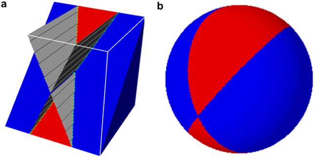
Missing wedge in limited-angle tomography. (a) Projections taken in a limited angular range provide information only in a region of Fourier space (blue) leaving a wedge-shaped region where no measurements are available (red). (b) Spherical representation of a volume affected by the missing wedge obtained by projecting the magnitude of the 3D Fourier Transform onto the unit sphere showing the separation between available and missing data.

For simplicity, we now introduce the ideas involved in comparing images with missing data in a one-dimensional case. In the example in Fig. 2, we consider two uni-dimensional functions v₁(x) and v₂(x) that have missing information represented by 0-valued segments. We model these functions as products with occluding masks m₁(x) and m₂(x) that are defined to be 1 in the regions where measurements are available and 0 in areas of missing information. We are now concerned with defining a metric to measure dissimilarity between v₁ and v₂ in a manner that is consistent with the missing data paradigm. This can be achieved if we restrict the comparison between the signals to regions where both are available, that is, where m₁(x) and m₂(x) are simultaneously non-zero (overlap region):

$$\mathrm{d}(v_1,v_2)=\int \parallel v_1\left(x\right)-v_2\left(x\right)\parallel m_1\left(x\right)m_2\left(x\right)\mathrm{d}x.$$ (1)

Without this restriction, regions where only one of the signals is available will still contribute to d(v₁, v₂) by an amount proportional to either ∥v₁(x∥ or ∥v₂(x)∥ depending on which signal is missing. Note that the extent of the overlap region m₁(x)m₂(x) may change for different sizes or relative position of the masks, effectively changing the size of the integration domain in Eq. (1). For reasons that will become evident in the next section, it is desirable to have a standardized measure of dissimilarity that does not depend on the size of the overlap region. This can be achieved by replacing d(v₁(x), v₂(x) with a normalized version that measures the average dissimilarity within the overlap region:

$$\mathrm{d}(v_1,v_2)=\frac{\int \parallel v_1\left(x\right)-v_2\left(x\right)\parallel m_1\left(x\right)m_2\left(x\right)\mathrm{d}x}{\int m_1\left(x\right)m_2\left(x\right)\mathrm{d}x}.$$

Fig. 2.

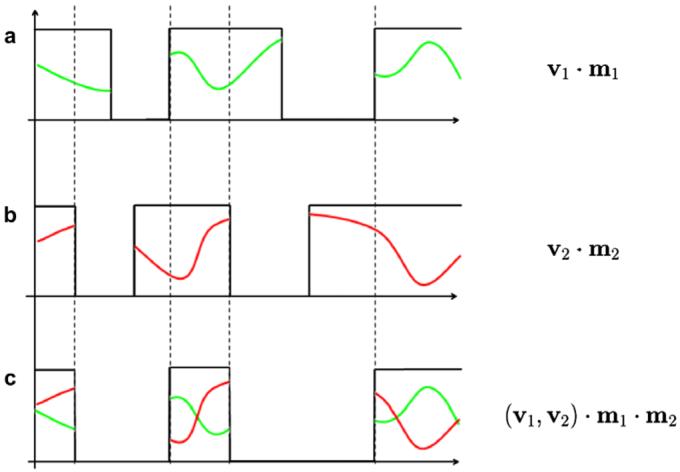
Measuring dissimilarity between partially occluded one-dimensional signals. (a) Missing data represented as product of signal v₁ with occluding mask m₁. (b) A second signal v₂ affected by a different mask m₂. (c) Computation of dissimilarity between both signals should be restricted to areas where both masks are non-zero.

We now extend these ideas to the case of signals that represent 3D volumes affected by the missing wedge. As mentioned before, we have chosen to carry out all computations in Fourier space where measured and missing information are naturally separated. Let V₁ and V₂ be two volumes reconstructed from limited-angle tomography having 3D complex Fourier Transforms ${\mathcal{F}}_1$ and ${\mathcal{F}}_2$, respectively. The missing wedge of each volume is represented by a 3D mask in reciprocal space ℳ_i=1,2 with value 1 in regions where frequency measurements are available and 0 in areas with no data coverage due to the limited tilt range. Strictly speaking, each tilted projection only contributes a thin slice of information in reciprocal space leaving a small wedge of missing data in between tilts. We assume that within a limited range of frequencies (usually given by a bandpass filter) the spacing between tilts can be neglected provided that the angular sampling is sufficiently fine. As in the one-dimensional case, we define the dissimilarity between the two volumes as:

$$\mathrm{d}(V_1,V_2)=\frac{{\int }_{\mathbf{f}\in \mathcal{B}}v\left(\mid {\mathcal{F}}_1\left(\mathbf{f}\right)-{\mathcal{F}}_2\left(\mathbf{f}\right)\mid \right){\mathcal{M}}_1\left(\mathbf{f}\right){\mathcal{M}}_2\left(\mathbf{f}\right)\mathrm{d}\mathbf{f}}{{\int }_{\mathbf{f}\in \mathcal{B}}{\mathcal{M}}_1\left(\mathbf{f}\right){\mathcal{M}}_2\left(\mathbf{f}\right)\mathrm{d}\mathbf{f}},$$ (2)

where v : ℝ → ℝ is a similarity kernel and comprises the range of relevant frequencies usually imposed by a bandpass filter in order to eliminate the unwanted contributions of low and high frequency components.² As noted before, the denominator in Eq. (2) makes the measurement independent of the size of the overlap region effectively measuring the average v-dissimilarity within the overlapping area. From now on we will use the square matching kernel v(x) = x² and in this case Eq. (2) will measure the average 2-norm of the difference between the Fourier Transforms in the overlapping region and within the frequency range . Note that minimization of the numerator in Eq. (2) in this case is equivalent to maximization of the usual cross-correlation coefficient after the images have been filtered to include only overlapping frequency components.

Sub-volumes extracted from reconstructions of different tilt series that were acquired under different conditions usually have dissimilar ranges of intensity making direct evaluation of Eq. (2) inappropriate as it will inevitably reflect these differences. This problem is also present in single-particle electron microscopy, and typically resolved by application of a normalization step (that forces zero mean and unit variance on all images) before evaluation of the dissimilarity score. For tomographic data however, the problem is more complex because the missing information in reciprocal space prevents the univocal determination of statistical image properties like the mean and the variance. For example, consider two uni-dimensional signals corresponding to the same function but affected by two different occluding masks. The variances of the partially occluded signals will be different because the occluding masks are different (even though the original signal is the exact same). Assuming that the signals are aligned to each other, one can restrict the computation of the variance only to include the overlap region and in this case both signals will have the same variance. Although this does not hold if the signals are not aligned, one would still expect true corresponding matches to yield better scores than those accounted for by scaling differences alone. We have then chosen to apply this type of normalization in our approach, which is equivalent to that implied in the use of constrained cross-correlation presented in Frangakis et al. (2002) and Förster et al. (2005, 2008).

Assuming this normalization scheme, the expression in Eq. (2) provides a formal framework for the generalization of dissimilarity measures previously proposed in the literature. The constrained cross-correlation function proposed in Frangakis et al. (2002) to measure dissimilarity between a volume with missing wedge and a reference with no missing wedge, can be obtained by substituting ℳ₂(f) = 1 in Eq. (2) and ignoring the integral in the denominator. The extension of the constrained correlation (Förster et al., 2008) to the case of two volumes affected by the missing wedge can also be derived from Eq. (2) by keeping the same integral in the numerator and eliminating the one in the denominator. Per the discussion in the previous section, the absence of this normalizing term can bias the alignment toward orientations that minimize the size of the overlap region ℳ₁(f)ℳ₂(f), by effectively reducing the extent of the integration domain. The measure of dissimilarity introduced in Schmid et al. (2006) can also be derived from Eq. (2) by removing the overlap term ℳ₁(f)ℳ₂(f) from the numerator and leaving the denominator unchanged. In this case, the varying size of the overlap region is correctly accounted for, but the integral in the numerator will include contributions from regions where either of the missing wedges is not zero, resulting in possibly biased alignment estimates.

In this section we have introduced a way of measuring similarity between volumes reconstructed from limited-angle tomography by treating the problem as the comparison of signals with missing data. The definition of dissimilarity in Eq. (2) constitutes the foundation for the subsequent analysis of image alignment and classification, it also provides a formal framework for the generalization of other measures proposed in the literature.

4. The 3D alignment problem

We are now concerned with aligning volumes, which involves finding the correct 3D rigid body transformation (rotation and translation) which when applied to the second volume minimizes the dissimilarity score. We let ${\Lambda }_{\mathcal{T}}\cdot {\Lambda }_{\mathcal{R}}$ be the linear operator that applies a rotation about the origin of three-dimensional space followed by a translation in ℝ³. Solving the alignment problem between V₁ and V₂ consists in finding the pair $\{{\mathcal{T}}_0,{\mathcal{R}}_0\}$ that minimizes the dissimilarity score defined in Eq. (2):

$$\{{\mathcal{T}}_0,{\mathcal{R}}_0\}=\underset{\mathcal{T}\in {\mathbb{R}}^3,\mathcal{R}\in SO\left(3\right)}{\arg \min }\mathrm{d}(V_1,{\Lambda }_{\mathcal{T}}\cdot {\Lambda }_{\mathcal{R}}\left(V_2\right)),$$ (3)

where SO(3) denotes the group of all possible 3D rotations about the origin. The success of the alignment routine is clearly dependent on the definition of dissimilarity used, which should measure the true dissimilarity between volumes regardless of the size and orientation of the missing wedge. Techniques that do not account for the missing wedge equally weight the measured and the missing data components in the two volumes, thus biasing the alignment result. Also the importance of weighting the dissimilarity score by the size of the overlapping region now becomes more clear. Without this weighting, the geometry of the overlapping region maybe conveniently altered resulting in an incorrect alignment.

Expanding the expression for $\mathrm{d}(V_1,{\Lambda }_{\mathcal{T}}\cdot {\Lambda }_{\mathcal{R}}\left(V_2\right))$ according to Eq. (2) yields:

$$\frac{{\int }_{\mathbf{f}\in \mathcal{B}}{\mid {\mathcal{F}}_1-{\mathrm{e}}^{-\mathrm{j}\mathbf{f}\mathcal{T}}{\Lambda }_{\mathcal{R}}\left({\mathcal{F}}_2\right)\mid }^2{\mathcal{M}}_1{\Lambda }_{\mathcal{R}}\left({\mathcal{M}}_2\right)\mathrm{d}\mathbf{f}}{{\int }_{\mathbf{f}\in \mathcal{B}}{\mathcal{M}}_1{\Lambda }_{\mathcal{R}}\left({\mathcal{M}}_2\right)\mathrm{d}\mathbf{f}},$$ (4)

where we have used the time shift property of the complex Fourier Transform, the fact that rotation and the Fourier Transform commute, and have dropped the variables of integration for simplicity of notation. Note that ℳ₂ is only affected by the rotational transformation ${\Lambda }_{\mathcal{R}}$ thanks to the shift-invariance property of the mask in reciprocal space.

In principle, solving the alignment minimization problem in Eq. (3) involves exhaustive searching of a six-dimensional parameter space (three for rotations and three for translations) in order to determine the transformation that minimizes this functional that could have multiple solutions corresponding to local minimizers. This is in fact how currently available techniques tackle this problem. Our algorithm for minimizing Eq. (3), however, circumvents the need for exhaustive search. Because alignment is used routinely throughout the classification and refinement stages described later, the reduction in computational time is very significant, thereby permitting the rapid and accurate processing of large sets of volumes. By taking a divide-and-conquer approach we break down the search into two three-dimensional problems each solved efficiently by using the convolution theorem in harmonic analysis. We first compute the rotation using Spherical Harmonics (SH), and then the translation using the convolution theorem in Fourier analysis. In the next section we describe this minimization approach in detail.

4.1. Minimizing the dissimilarity score

The separation of the original 6 degree-of-freedom problem into two 3 degree-of-freedom problems is achieved by working with a translationally invariant version of Eq. (3) obtained by substituting the complex Fourier Transforms by their magnitudes. We then project these images onto the unit sphere, and transform the problem of finding the optimal rotation between two 3D volumes into finding the rotation between their spherical images. By using the convolution theorem in Spherical Harmonics we readily obtain the rotational transformation that produces the best match. We then go back to the original form of Eq. (3) and find the translational transformation using the convolution theorem in Euclidean space. A key property of our approach is that the representation of the missing wedge is preserved at all times allowing missing data to be modeled as occluding masks throughout the process.

Substituting the Fourier Transforms by their magnitudes in Eq. (4) we obtain a translationally invariant formulation of the alignment problem where the rotation is now the only unknown:

$${\mathcal{R}}_0=\underset{\mathcal{R}\in SO\left(3\right)}{\arg \min }\frac{{\int }_{\mathbf{f}\in \mathcal{B}}{(\mid {\mathcal{F}}_1\mid -{\Lambda }_{\mathcal{R}}\mid {\mathcal{F}}_2\mid )}^2{\mathcal{M}}_1{\Lambda }_{\mathcal{R}}\left({\mathcal{M}}_2\right)\mathrm{d}\mathbf{f}}{{\int }_{\mathbf{f}\in \mathcal{B}}{\mathcal{M}}_1{\Lambda }_{\mathcal{R}}\left({\mathcal{M}}_2\right)\mathrm{d}\mathbf{f}}.$$ (5)

Here we have used the fact that ${\Lambda }_{\mathcal{R}}$ and the magnitude of the Fourier Transforms commute, i.e., $\mid {\Lambda }_{\mathcal{R}}\left({\mathcal{F}}_2\right)\mid ={\Lambda }_{\mathcal{R}}\left(\mid {\mathcal{F}}_2\mid \right)$. The next step is to convert volumes into spherical images and recover the rotation by taking advantage of the spherical convolution theorem. Denoting with S² = {p ∈ ℝ³|∥p∥ = 1} use the set of points on the unit sphere, we use the parametrization in spherical coordinates η = η(Θ, ϕ) with colatitude Θ ∈ [0, π] and longitude ϕ ∈ [0, 2π] to represent points on S² as:

$$p=\eta (\theta ,\varphi )=(\cos \left(\varphi \right)\sin \left(\theta \right),\sin \left(\varphi \right)\sin \left(\theta \right),\cos \left(\theta \right)).$$

We associate to each volume $\mid {\mathcal{F}}_i\mid$ an image defined on the unit sphere f_i(η) : S² → ℝ obtained by integrating along rays though the origin:

$$f_i\left(\eta (\theta ,\varphi )\right)={\int }_{{\rho }_a}^{{\rho }_b}\mid {\mathcal{F}}_i\left(\rho \eta (\theta ,\varphi )\right)\mid \mathrm{d}\rho ,$$

where ρ is the radial variable in spherical coordinates and (ρ_a, ρ_b) defines the range of frequencies passed by the bandpass filter. This projection of the magnitude of the 3D Fourier Transform into the lower dimensional space of the unit sphere maintains the geometry of the missing wedge, see Fig. 1. That is, if a voxel falls in the missing wedge region then all other voxels in a straight line through the origin will fall in the missing wedge as well. Because of this property, we can continue to use the formulation introduced in Section 3 to represent the missing wedge with binary masks now defined on the unit sphere m_i=1,2 : S² → {0, 1}. The alignment problem between the spherical images f₁ and f₂ is now defined as follows:

$${\mathcal{R}}_0=\underset{\mathcal{R}\in SO\left(3\right)}{\arg \min }{\mathrm{d}}_s(f_1,{\Lambda }_{\mathcal{R}}\left(f_2\right)),$$ (6)

where ${\Lambda }_{\mathcal{R}}$ is the rotation operator as before and the dissimilarity in this new spherical representation is:

$${\mathrm{d}}_s(f_1,{\Lambda }_{\mathcal{R}}\left(f_2\right))=\frac{{\int }_{\eta \in S^2}{(f_1-{\Lambda }_{\mathcal{R}}{f}_2))}^2{m}_1{\Lambda }_{\mathcal{R}}\left(m_2\right)\mathrm{d}\eta }{{\int }_{\eta \in S^2}{m}_1{\Lambda }_{\mathcal{R}}\left(m_2\right)\mathrm{d}\eta }.$$

It is now convenient to introduce the spherical convolution operation, which is defined between two spherical images f₁ and f₂ and assigns to each 3D rotation the following scalar value:

$$(f_1\star f_2)\left(\mathcal{R}\right)={\int }_{\eta \in S^2}{f}_1\left(\eta \right){\Lambda }_{\mathcal{R}}\left(f_2\left(\eta \right)\right)\mathrm{d}\eta .$$ (7)

This definition can be used to express ${\mathrm{d}}_s(f_1,{\Lambda }_{\mathcal{R}}\left(f_2\right))$ as a function of expressed in terms of spherical convolutions:

$${\mathrm{d}}_s\left(\mathcal{R}\right)=\frac{f_1^2{m}_1\star m_2-2f_1{m}_1\star f_2{m}_2+m_1\star f_2^2{m}_2}{m_1\star m_2}.$$ (8)

The reason this is important is that the spherical convolution operation can be computed efficiently as shown below.

In classical Fourier analysis square-integrable periodic functions in the line can be written as a series of complex exponential functions {e^ikx}_k∈Z, which forms an orthonormal basis for that space. Similarly, spherical harmonic functions form an orthonormal basis for the space of functions defined on the unit sphere. Any square-integrable function f(η) defined on S² with bandwidth B ∈ can be expanded as a series:

$$f\left(\eta \right)=\sum _{l=0}^{B-1}\sum _{m=-l}^l{\widehat{f}}_{lm}{Y}_l^m\left(\eta \right),$$ (9)

where $Y_l^m\left(\eta \right)$ are the spherical basis functions and f̂_lm are the coefficients of the Spherical Fourier Transform satisfying f̂_lm ≃ 0 for l ≥ B (see MacBobert, 1927 for details).

Similarly, functions defined on SO(3) can also be decomposed as a series of basis functions leading to the definition of a Fourier Transform on SO(3). In analogy to the Convolution Theorem in classical Fourier Analysis, SO(3) Fourier Transform coefficients of the spherical convolution can be obtained directly from pointwise multiplication of the Spherical Fourier Transform coefficients of the two spherical images being convolved. By computation of an inverse SO(3) Fourier Transform, the spherical convolution can be efficiently evaluated for all rotations simultaneously, see Kostelec and Rockmore (2003) and Makadia and Daniilidis (2006) for details. Using this result we can compute ${\mathrm{d}}_s\left(\mathcal{R}\right)$ in Eq. (8) by evaluation of four spherical convolutions (namely $f_1^2{m}_1\star m_2$, f₁m₁★f₂m₂, $m_1\star f_2^2{m}_2$, and m₁★m₂), and obtain the alignment solution, ${\mathcal{R}}_0$, by finding the coordinates corresponding to its minimum value.

We now go back to the full 3D dissimilarity measure in Eq. (3) to compute the translation ${\mathcal{T}}_0$ while keeping the rotation fixed at ${\mathcal{R}}_0$. The denominator in this case is constant and the translation can be obtained from:

$${\mathcal{T}}_0=\underset{\mathcal{T}\in {\mathbb{R}}^3}{\arg \min }{\int }_{\mathbf{f}\in \mathcal{B}}{\mid {\mathcal{F}}_1-{\mathrm{e}}^{-\mathrm{j}\mathbf{f}\mathcal{T}}{\Lambda }_{{\mathcal{R}}_0}\left({\mathcal{F}}_2\right)\mid }^2{\mathcal{M}}_1{\Lambda }_{{\mathcal{R}}_0}\left({\mathcal{M}}_2\right)\mathrm{d}\mathbf{f}.$$

We can now move the overlap term ${\mathcal{M}}_1{\Lambda }_{{\mathcal{R}}_0}\left({\mathcal{M}}_2\right)$ inside the 2-norm and define new volumes Ṽ_i=1,2(x) as follows:

$$\begin{array}{c}\hfill {\tilde{V}}_1\left(\mathbf{x}\right)={\mathcal{F}}^{-1}\left({\mathcal{F}}_1{\mathcal{M}}_1{\Lambda }_{{\mathcal{R}}_0}\left({\mathcal{M}}_2\right)\right),\hfill \\ \hfill {\tilde{V}}_2\left(\mathbf{x}\right)={\mathcal{F}}^{-1}\left({\mathcal{M}}_1{\Lambda }_{{\mathcal{R}}_0}\left({\mathcal{F}}_2{\mathcal{M}}_2\right)\right).\hfill \end{array}$$

These correspond to filtered versions of the original volumes that only retain frequency components within the overlap region of both missing wedges (after application of the rotational transformation given by the alignment solution). Substituting the above expressions and applying Parseval’s Theorem we obtain the translational alignment formula in real space:

$${\mathcal{T}}_0=\underset{\mathcal{T}\in {\mathbb{R}}^3}{\arg \min }\int {({\tilde{V}}_1\left(\mathbf{x}\right)-{\tilde{V}}_2(\mathbf{x}-\mathcal{T}))}^2\mathrm{d}\mathbf{x},$$

which is equivalent to solving

$${\mathcal{T}}_0=\underset{\mathcal{T}\in {\mathbb{R}}^3}{\arg \min }\int {\tilde{V}}_1\left(\mathbf{x}\right){\tilde{V}}_2(\mathbf{x}-\mathcal{T})\mathrm{d}\mathbf{x},$$

efficiently computed using the convolution theorem in Euclidean space. At this point we have recovered the pair $\{{\mathcal{T}}_0,{\mathcal{R}}_0\}$ that solves the full 3D alignment problem without need for exhaustive search.

Note that ${\mathcal{R}}_0$ is the solution to the spherical alignment problem Eq. (6) and not necessarily a solution to the 3D problem in Eq. (5). Although the modulo operation and the dimensionality reduction implied by the radial projection give a way of efficiently finding a minimizer, it also inevitably introduces ambiguity to the solution. This ambiguity can be resolved easily by evaluating the 3D dissimilarity in Eq. (2) at the top ranked local minima within the ${\mathrm{d}}_s\left(\mathcal{R}\right)$ volume and choosing the one that gives the minimum value for the 3D matching score. Also, the accuracy of the rotation estimate ${\mathcal{R}}_0$ is dictated by the sampling of the SH grid and the number of coefficients used in the SH expansion. Therefore, we further refine both ${\mathcal{T}}_0$ and ${\mathcal{R}}_0$ by locally minimizing Eq. (2) using Powell’s algorithm (Press et al., 1996) which is an improved version of the classic conjugate directions algorithm.

Prior to the evaluation of all alignment computations, sub-volumes have to be normalized to eliminate the contribution of unwanted intensity variations (see Section 3). Our strategy of imposing both images to have unit variance within the overlap region, requires the normalization to be done separately for each 3D rotation, because the overlap region changes as volumes are rotated. Nonetheless, this can be easily incorporated into the alignment routine described in this section by simply substituting f₁ and f₂ in Eq. (8) with their normalized versions $\frac{f_1}{\sqrt{f_1^2{m}_1\star m_2}}$ and $\frac{f_2}{\sqrt{m_1\star f_2^2{m}_2}}$ yielding the corrected spherical dissimilarity:

$$\stackrel{‒}{{\mathrm{d}}_s}\left(\mathcal{R}\right)=\frac{2\left(1-\frac{f_1{m}_1\star f_2{m}_2}{\sqrt{f_1^2{m}_1\star m_2}\sqrt{m_1\star f_2^2{m}_2}}\right)}{m_1\star m_2},$$

that can be evaluated rapidly by computation of four spherical convolutions as before.

In this section we have introduced an efficient and accurate way of solving the alignment problem presented in Section 4 between volumes affected by a missing wedge. This procedure will be used routinely as one of the critical components for the refinement alignment-classification loop presented in Section 6.

5. Classification of volumes affected by the missing wedge

For successful interpretation of images of complex biological assemblies recorded at very low doses (and therefore low signal-to-noise ratios), we need a robust classification strategy for averaging. This is extremely important for making sure that averages are computed strictly from homogeneous sets of volumes. In practice, some degree of true density variability will be sacrificed in favor of improving the signal-to-noise ratio. The value of classification techniques is that of providing a glimpse of the landscape of conformations so that an educated decision can be made about the level of averaging that is most appropriate. As in the alignment procedure, in order to guarantee a correct result, the classification strategy has to take into account the fact that volumes are affected by the missing wedge. Note that the missing wedge is likely to be just one of many factors (e.g., different defocus, radiation damage, etc.) contributing to image heterogeneity besides genuine structural differences. In the absence of a complete understanding and modeling of their interaction, we can only attempt to study the contribution of each factor in isolation, by conducting artificial and real experiments where ground-truth is available and validation is possible.

Throughout this section we assume volumes to be in a fixed orientation, however, the missing wedge in each of them may be arbitrarily oriented. In general, classification involves partitioning a set of volumes into clusters so that volumes within each group satisfy some proximity criteria. Approaches to data clustering have usually two components: a metric to measure dissimilarity and a grouping or classification strategy. In our case, the metric is defined between 3D volumes which are represented as high-dimensional vectors with as many dimensions as there are voxels in each volume. In order to facilitate the analysis, a dimensionality reduction strategy is usually required to identify the most important variations within the high-dimensional data and at the same time minimize the influence of the noise. The metric can then be defined in the reduced space and a variety of grouping techniques such as k-means or hierarchical clustering may be applied.

Multivariate statistical analysis techniques for 3D classification in real space (Walz et al., 1997; Winkler, 2006) are computationally attractive and effective in reducing the dimensionality of the data. However, the metrics implied in the analysis do not account for the missing wedge because measured and missing information are not distinguishable in real space, resulting in inaccurate classification results. Metrics that account for the missing wedge are thus required in order to guarantee a meaningful classification, but their use is less computationally attractive as they require explicit evaluation of all-versus-all dissimilarities.

Our approach to clustering uses the metric introduced in Section 3 that fully accounts for the missing wedge by exclusively comparing the frequencies within a band where measurements from both volumes are available. The dimensionality reduction strategy in this case is implicit in the definition of the metric (Eq. (2)), as integrals in reciprocal space are restricted to a small frequency region determined by the pass-band of the filter . Although this typically results in a reduction factor worse than those achieved by multivariate statistical analysis techniques, it is good enough to permit a meaningful discrimination between sets of images. After explicit evaluation of all-versus-all dissimilarities using Eq. (2) we apply a Hierarchical Ascending Classification technique using Ward’s criteria (Ward, 1963) that minimizes the internal variance of classes while at the same time maximizes the inter-class variance. Note however, that the sorting strategy within our framework is viewed as a modular entity that could easily be exchanged to accommodate other classification algorithms also based on the analysis of dissimilarities. Because we compute dissimilarities with a metric that fully takes the missing data into account, results will not to be biased by the presence of the missing wedge regardless of the particular clustering strategy being selected. After building the classification tree, a fixed number of classes are obtained by thresholding the tree at the appropriate level. We now have a partition of the set of input volumes and a class average can be associated to each cluster. Since we are averaging volumes affected by the missing wedge, the sum has to be carried out in Fourier space and be properly normalized by the actual number of contributing volumes at each voxel. This has been pointed out in the literature before and it is critical to prevent regions with missing information to be averaged with areas of useful information.

6. Iterative refinement with simultaneous alignment and classification

At this point we have introduced separate methods for both the alignment and classification of volumes affected by the missing wedge. We now combine these into a single iterative procedure aimed at solving the general classification-alignment problem restated as follows. Given a set of volumes V_n=1,...,N that correspond to noisy and randomly rotated copies affected by the missing wedge of K different conformations, the goal is to partition and align the set V_n in order to obtain class averages R_k=1,...,K representing each of the K conformations.

We solve this problem using a variant of the alignment-through-classification technique mentioned in Section 2 to automatically detect and progressively refine the class averages R_k. The procedure has the following steps:

1. Assume the alignment of V_n’s is fixed and build the hierarchical classification tree to obtain class averages R_k as described in Section 5.

2. Refine each class average R_k and align all refined averages to a common frame.

3. Align all V_n’s to the refined and aligned class averages generated above using the methods described in Section 4.

4. Update the alignment of each V_n to that of the best matching R_k and go back to step (i).

Assuming the V_n’s are not initially pre-aligned, the first iteration of the algorithm will group volumes that are similar and also have the same orientation and relative position within the boxed region. This partitioning will result in multiple class averages for each real conformation with each version representing a different rotated and translated representation. As a consequence, a large number of clusters maybe needed in this first iteration to make sure that most unique conformations are captured. Depending on the total number of volumes N, initial classes may not be statistically significant and the use of a pre-alignment step maybe required to effectively reduce the number of distinct initial configurations as described in Section 2. In subsequent iterations however, the classification step will group volumes exclusively by image similarity (i.e., regardless of orientation and position within the extracted volumes) requiring the use of fewer classes when thresholding the hierarchical classification tree in step (i).

For the refinement of class averages in step (ii) we use the algorithm for aligning sets of images presented in Penczek et al. (1992) to guarantee that volumes within a class are optimally aligned. An outlier rejection step (to leave out volumes with low matching scores from the refined averages) may be included at this stage. The rejection criteria may be based on a dissimilarity threshold or percentage of rejected volumes as a fraction of the total number volumes contributing to the average. After refinement is done all class averages are aligned to a common reference, e.g., the most populated class. This step is critical for the assignment of volumes to the closest reference done in the next step (iv), making the result less susceptible to eventual alignment errors. For example, if a volume is assigned to the wrong reference because the dissimilarity to another reference is slightly smaller, the global alignment will still be correct because references are all aligned to each other. Also worth noting is that intermediate class averages formed by combination of volumes affected by the missing wedge, may still have a missing region of information which is not necessarily wedge-shaped. The extent of this region can be obtained by combining the missing wedge masks of each particle contributing to the average in the proper orientation, producing a new missing data mask in reciprocal space, ℳ_i, that can be used for the alignment between class averages.

As alignments get progressively better with the iterations, volumes within a class will align better with respect to each other (as a result of the successive intra-class refinement steps) and they will also align better to volumes in other classes because class averages are, in turn, aligned to each other. This effect can be quantified by computing the square root of the sum of squares over all elements (Frobenius norm) of the dissimilarity matrix used to compute the hierarchical classification tree in step (i). This is in fact one of the quantitative indicators we monitor in the experiments presented next, in order to evaluate the performance of the algorithm. Note that the goal of the iterative alignment procedure (Penczek et al., 1992) for aligning heterogeneous sets of images is precisely the minimization of this quantity, but unlike the approach presented here, it requires the selection of a reference for initialization potentially resulting in biased averaging results (see Section 2). The loop is terminated when no significant changes are observed in the class averages.

7. Validation experiments

To analyze the performance of our framework for alignment and classification, we present here results both with artificial phantoms and experimental tomographic data obtained from plunge frozen GroEL specimens. Because “ground-truth” is available in both cases, we can quantitatively evaluate the correctness of our framework and study its behavior for different parameter settings. All of the analysis in this section was carried out with sub-volumes that were 64 × 64 × 64 in size and a raised cosine spherical image mask was applied at the edge before all FFT calculations. Each sub-volume has a tilt axis and associated tilt range that are used to compute the 3D wedge mask in reciprocal space. Spherical Harmonics calculations were done with the SOFT package (Kostelec and Rockmore, 2003) using a bandwidth of B = 64 equivalent to having a 128 × 128 × 128 sampling grid for the three Euler angles. A bandpass filter with (.05, .35) cutoffs (as fractions of the sampling frequency) was used for the evaluation of all dissimilarities. The code for the experiments was parallelized to take advantage of the high performance computational capabilities of the Biowulf Linux cluster at the National Institutes of Health, Bethesda, MD.

7.1. Validation with phantoms

Two sets of analyses are presented in this section, one to measure the performance of the alignment routine presented in Section 4 and the other to study the performance of the alignment-classification loop presented in Section 6. In both cases, 3D maps representing distinct geometric conformations are generated and subject to a process intended to mimic electron tomographic imaging. The steps involved in this process are:

• -Computation of a series of projection images by tilting the 3D map along the Y axis in a ±w degree range.
• -Addition of zero-mean random noise to each projection and application of a random in-plane shift in a ±p pixel range in each dimension to simulate tilt series alignment errors. The magnitude of the added noise and image shifts attempt to mimic those encountered in the real tomograms as closely as possible.
• -Computation of the 3D reconstruction from the noisy and misaligned tilt series using the Algebraic Reconstruction Technique (ART).

This process is repeated several times for each 3D phantom by changing the noise, tilt range and alignment parameters in order to simulate different experimental conditions.

To study the performance of the alignment technique presented in Section 4, we use a non-symmetric phantom model consisting of three arms joined at one end. For different noise and tilt range combinations, we produced ten randomly rotated and shifted copies of the phantom and subjected each to the image generation model described above. We then computed all pairwise alignments between reconstructed volumes and compared the results to ground-truth values by measuring the square root of the sum of squares over all elements of the linear transformation matrices. In Fig. 3 we show the average alignment error plots obtained using the technique presented in Section 4 and compare the results to the case with no missing wedge compensation. Alignment performance in the absence of missing wedge correction degrades rapidly for tilt ranges smaller than ±70° and modest noise levels. In contrast, compensation for the missing wedge using our approach, allows reasonably accurate alignment even when the data is collected using tilt ranges as low as ±55°, and results in better tolerance to noise. Note that the results shown above are to some extent dependent on the shape of the phantom selected for the experiments, e.g., they will get better if we use a symmetric phantom configuration thanks to the added redundancy. In general, the success of the alignment routine depends on the relative size and location of the missing wedge with respect to important image features in reciprocal space. Under certain circumstances, the available information in Fourier space may simply be not enough to allow the correct alignment of volumes (even in the noise-free case) because the features needed for alignment are masked by the missing information.

Fig. 3.

Average alignment error for different sizes of missing wedge and noise level added to projections. (a) Using cross-correlation alignment without accounting for the missing wedge. Total mean square error = 3.72. (b) Using the technique introduced in Section 4. Total mean square error = 1.37.

To illustrate the potential implications of our alignment routine, we built a threefold symmetrical phantom with a simulated extension in only one of the arms (Fig. 4) to test whether pseudo-symmetric or closed related but distinct structures could be aligned properly. Seventy randomly oriented copies of this phantom were generated and subjected to the image generation process using forty projections in a ±60° tilt range. We aligned all volumes in the set both with and without correction for the missing wedge and computed the resulting volume averages as shown in Fig. 4. The results unambiguously demonstrate the importance of wedge correction since in the absence of this step, the extension in one of the arms is erroneously spread to the other two arms due to frequent alignment errors, while properly accounting for the missing wedge allows recovery of the correct structure.

Fig. 4.

Effect of alignment errors due to the missing wedge in volume averaging. (a) Starting phantom model. (b) Average of 70 volumes derived without consideration of the missing wedge results in spreading of the unique feature to all three arms due to frequent alignment errors. (c) Average of 70 volumes obtained using our procedure for alignment that accounts for the missing wedge; the feature is correctly recovered in only one of the arms.

To rigorously evaluate the performance of the iterative classification-alignment procedure presented in Section 6 we used five phantom models representing distinct conformations labeled as M, D1, D2, T1, and T2 as shown in Fig. 5. These configurations were selected to produce closely related objects with a high degree of similarity, but nevertheless with distinct structural differences such as variations in angular spread or in the number of extending arms. More complex configurations were built by adding an extra piece of density to simpler configurations, e.g., M vs. D1, D1 vs. T1, etc. Separating these phantom configurations by classification poses a challenging problem given the high degree of similarity between them, the limited SNR and the presence of the missing wedge. For example, it is not unusual that the missing wedge will align to one of the arms of the D1 configuration, making the volume affected by the missing wedge appear undistinguishable from one of the M configuration that has a single arm. We generated a series of 550 volumes (75 M, 100 D1, 125 D2, 125 T1, 100 T2, and 25 pure noise) corresponding to copies of the original phantom configurations randomly oriented and shifted, subjected to the mock tomography imaging described above using 40 projections in a ±60° range. We tested two different scenarios: noise was added to the projections such that SNR = 0.04 and SNR = 0.018 at each projection before reconstruction, and in-plane shifts were applied of ±2.5 and ±5 pixels, respectively, see Fig. 6. Given the unlabeled set of 550 volumes, our goal is to recover the starting set of conformations M, D1, D2, T1 and T2 by using the iterative refinement technique introduced in Section 6. Fixing the number of classes at six for all iterations, we executed the algorithm in an unsupervised mode until classes did not change significantly. Fig. 7 shows the classification confusion matrices for both experimental settings after the first iteration and at steady state. The confusion matrix shows the assignment of volumes into classes I, II, III, IV, V and VI in correspondence with the ground-truth M, D1, D2, T1, T2 and noise. For the first case (SNR = 0.04 and ±2.5 pixel shifts) the confusion matrix converges to the unit diagonal after five iterations showing the successful separation of volumes into the original classes. When the SNR is degraded to 0.018 and the tilt series alignment error increased to ±5 pixels, not all conformations can be successfully separated. In particular, volumes generated from configurations D1 and D2 become indistinguishable given the high degree of similarity between the initial configurations and the increased noise conditions. This shows that distinguishing very similar configurations may be possible under minimum SNR requirements but will likely fail if these conditions are not met.

Fig. 5.

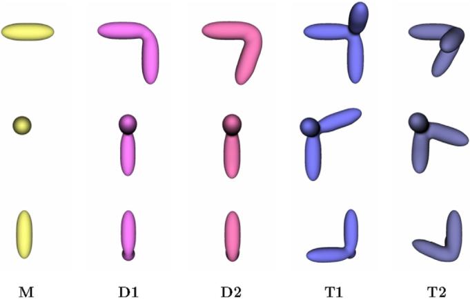
Phantom models used for validation of our classification strategy (X, Y, Z views). Configurations were designed to be similar to each other to explore performance of the classification routine in separating distinct conformations for a range of related structures.

Fig. 6.

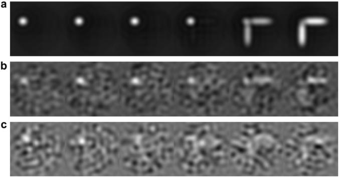
Reconstructions for the T1 phantom configuration using two different levels of noise. (a) Sequential slices of original T1 phantom. (b) Sequential slices of bandpass filtered reconstruction generated with noise added to 40 projections in ±60° range with SNR = 0.04 and random shifts of ±2.5 pixels. (c) Sequential slices of bandpass filtered reconstruction from 40 projections in ±60° range with SNR = 0.018 and ±5 pixel shifts.

Fig. 7.

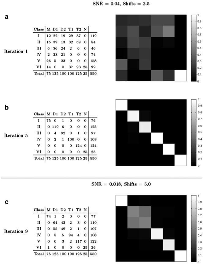
Classification results as confusion matrices on the phantom experiment for two experimental conditions. (a) Classification results after the first iteration of the algorithm for SNR = 0.04 and tilt alignment errors of ±2.5 pixels. (b) Result after five iterations shows successful separation of the five phantom configurations M, D1, D2, T1 and T2. (c) Classification results after nine iterations for SNR = 0.018 and alignment shifts of ±5 pixels. Most configurations can still be correctly separated, except D1 and D2 which become indistinguishable from one another due to the very high noise level.

7.2. Validation with GroEL

Purified GroEL (1 mg/ml) was mixed with 5 nm colloidal gold, applied to home-made thin holey carbon grids and vitrified using a Vitrobot device (FEI Company, OR). Imaging was performed at liquid nitrogen temperatures using a Polara field emission gun electron microscope (FEI Company, OR) equipped with a 2K × 2K CCD placed at the end of GATAN GIF 2002 postcolumn energy filter (GATAN, Pleasanton, CA) that was operated in the zero-energy-loss mode with a slit width of 30 eV. The microscope was operated at 300 kV and a magnification of 34,000×, giving an effective pixel size of about 4.1 Å at the specimen level. Low-dose single-axis tilt series were collected at underfocus values of about 5 μm. The angular range of the tilt series (≃100 images) was from -70° to +70° at increments chosen according to the cosine rule (2° at 0°). The cumulative dose of the tilt series was less than 80 e/Ų. Tilt series were aligned with gold markers using Inspect3D (FEI Company, OR) and reconstructed using algebraic reconstruction techniques. Fig. 8 shows a typical tomographic slice from a reconstructed volume. A set of 345 GroEL particles were extracted from six different tomograms, noting the precise tilt range and orientation with respect to the tilt axis in order to determine the geometry of the wedge mask used in our formulation. The effective tilt range for each of the six tilt series we used was (-70, 63), (-70, 65), (-70, 54), (-70 48), (-70, 59), and (-70, 63) after elim-high-tilt projections with poor contrast.

Fig. 8.

Slices of raw tomogram of GroEL. (a) 8.2 nm thick overview slice obtained by re-projection of 20 consecutive slices of the original reconstruction. (b) 4.1 Å thick slices (no re-projection) of individual particles extracted for analysis.

We first tested the classification algorithm presented in Section 5 before applying any alignment correction (missing wedges in this case have different extents but are all aligned in the vertical orientation). Fig. 9(a) shows a simplified diagram of the resulting hierarchical ascending classification tree of all 345 volumes. Images represented in the tree correspond to central slices through the averaged volumes at the corresponding branch. Characteristic GroEL top and side views are grouped together in homogeneous clusters while others (likely corresponding to intermediate views or damaged/incomplete molecules) are successfully separated. In Fig. 9(b) we repeated the classification experiment now randomizing the orientation of particles (and consequently that of the missing wedge) also showing that reasonable separation can be achieved.

Fig. 9.

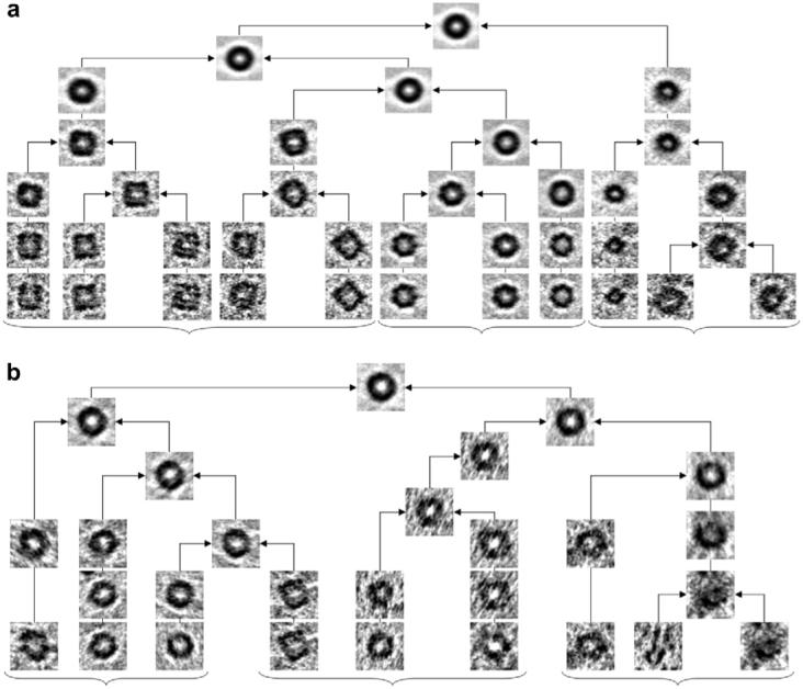
Simplified hierarchical classification tree for the 345-particle GroEL dataset showing successful clustering of volumes affected by the missing wedge. Each node of the tree corresponds to a three-dimensional volume (that we represent by its central slice) obtained by averaging the child nodes. (a) All volumes have a missing wedge with the same orientation (perpendicular to the page) but with different extents since they were extracted from tomograms with differing tilt ranges. We only show a handful of representative transitions extracted from the full hierarchical tree. At the lowest level shown, partial averages clearly show visually homogeneous clusters corresponding to side views (group to the left), top views (middle group), and intermediate or damaged/incomplete particles (group to the right). Branches merge up gradually, grouping most similar volumes first until all 345 particles become one class (top node). (b) Classification results after volumes have been randomly rotated to shuffle the orientation of the missing wedges. Top and side views are still successfully separated but now appear interchanged: top views is the group to the left, and side views is the group in the middle. Note that the middle group contains averages of side-view particles but now viewed from the top (rightmost sub-group within the middle group). The group to the right again shows and heterogeneous mix likely corresponding to damaged or incomplete particles.

Next, we analyze the performance of the iterative classification-alignment procedure of Section 6. Keeping the number of classes fixed at five, we ran the iterative procedure in an unsupervised mode until convergence was achieved. In Fig. 10 we show the evolution of the class averages for iterations 1 (a) and 10 (b) of the refinement algorithm. In the absence of classification, the average of all sub-volumes will resemble that of the most populated class in Fig. 10 (a, fourth class) which shows none of the characteristic features of GroEL, and therefore will render subsequent alignment rounds ineffective causing the procedure to get stuck in a local minima. As a way of quantifying the improvement achieved by the iterative procedure, we monitored three different and independent performance indicators:

1. The first indicator measures the relative success of the refinement routine in reducing the sum of all-versus-all dissimilarities as described in Section 6. This quantity measures two components simultaneously. One reflects the accuracy of the intra-class alignment as an indicator of how well volumes are aligned within homogeneous classes and the second reflects how well the different classes are aligned to each other. Numeric evaluation of this indicator is equivalent to the computation of the Frobenius norm of the dissimilarity matrix.

2. As a second indicator, we measured the cross-correlation coefficient of the average map obtained at each iteration with a 6 Å map of GroEL, filtered to 20 Å obtained from single-particle analysis by Ludtke et al. (2004). As the average map gets progressively better with the iterations, this quantity is expected to increase.

3. As a third indicator, we tracked the resolution of the average map as given by the Fourier Shell Correlation, which is also expected to improve with more iterations.

Fig. 10.

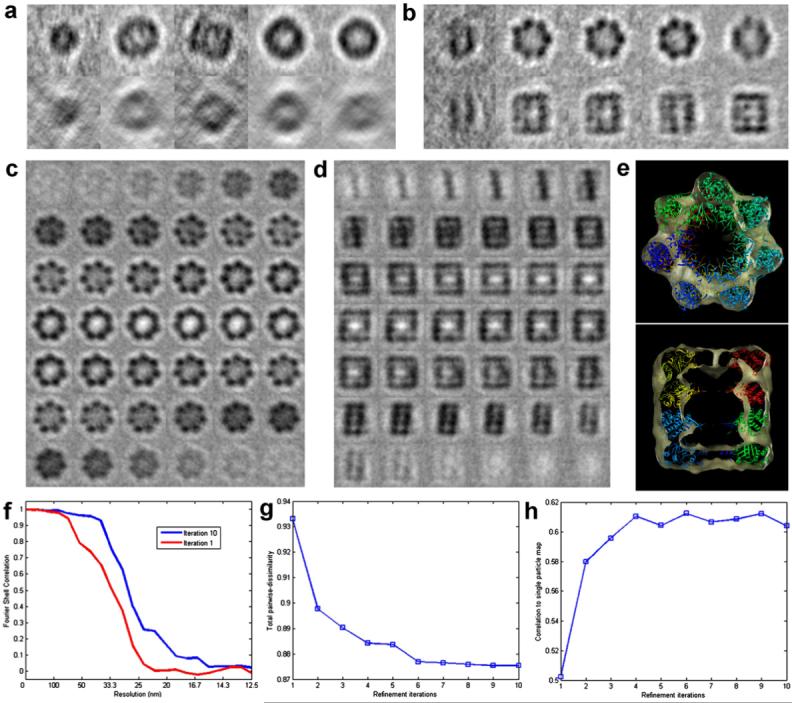
Iterative classification and alignment refinement results for GroEL. (a and b) Projection views in two orthogonal directions of five initial class averages (a) and after 10 rounds of refinement (b). (c and d) Consecutive sections of the 3D map obtained after 10 rounds of refinement showing typical low-resolution features of GroEL and clear evidence of the sevenfold symmetry. No symmetry was applied at any stage of image processing. (e) Docking of X-ray coordinates into GroEL map obtained after ten refinement iterations. Quantitative performance plots of the refinement procedure showing the improvement with iterations for three numerical indicators: (f) Fourier Shell Correlation plots, (g) Frobenius norm of all-versus-all dissimilarity matrix, (h) and cross-correlation coefficient of the averaged map to a map of GroEL at 20 Å, obtained by filtering the 6 Å reconstruction reported by Ludtke et al. (2004).

Fig. 10(c) and (d) shows two orthogonal montages of slices corresponding to the average map after 10 iterations and (e) the fitting of the X-ray coordinates. The results for the three performance indicators are presented in Fig. 10(f)-(h) showing that all plots are consistent with the expected results. The Frobenius norm of the dissimilarity matrix decreases rapidly during the first iterations showing the ability of the algorithm to successfully separate homogeneous groups of images (by virtue of gradual improvement of alignments) and converges asymptotically to its final value with more iterations. The same behavior is observed for the index measuring cross-correlation of our average map to the experimentally determined, higher-resolution map. The Fourier Shell Correlation plots are also consistent with the expected increase in resolution as alignments get better with the iterations, and converge to a value of ≃27 Å as determined by the .5 Fourier Shell Correlation criteria for a map obtained by combining 230 volumes (out of the initial 345). We note that no assumptions about symmetry were used at any stage of the analysis.

8. Concluding remarks

Averaging techniques in single-particle analysis have had great success in achieving high-resolution despite the low signal-to-noise ratios typical of electron microscopic images. In tomography however, the computational load required to process three-dimensional data, the need to deal with the missing wedge of information in reciprocal space, and the lack of tools to study variability have prevented the emergence of equivalent techniques that are successful. Here, we presented a framework for simultaneous alignment, classification and averaging of volumes obtained from electron tomography that overcomes these difficulties and provides a powerful tool for high-resolution and variability analysis of tomographic data significantly extending recent progress in the field. By regarding the missing wedge as an occluding mask, we are able to successfully align and classify volumes using only regions that contain common information ignoring the areas of missing data. We have shown the performance of our approach using both synthetic and real examples. We have also addressed what likely is the biggest hurdle in processing of large collections of volumes, which is the computational load required by the three-dimensional alignment procedure. The application of these image analysis strategies for investigation of structure and conformational variation of molecular multi-protein complexes represents a further step toward the long-term goal of understanding protein-protein interactions in the complex milieu of cells and viruses at atomic resolution.

References

- Bartesaghi A, Sprechmann P, Randall G, Sapiro G, Subramaniam S. Classification and averaging of electron tomography volumes; 4th IEEE International Symposium on Biomedical Imaging: From Nano to Macro; Washington, DC, USA. 2007.pp. 244–247. [Google Scholar]
- Crowther RA. In: The Molecular Replacement Method. Rossmann MG, editor. Gordon & Breach; New York: 1972. pp. 173–178. [Google Scholar]
- Förster F, Medalia O, Zauberman N, Baumeister W, Fass D. Retrovirus envelope protein complex structure in situ studied by cryo-electron tomography. Proceedings of the National Academy of Sciences of the United States of America. 2005;102(13):4729–4734. doi: 10.1073/pnas.0409178102. [DOI] [PMC free article] [PubMed] [Google Scholar]
- Förster F, Pruggnaller S, Seybert A, Frangakis AS. Classification of cryo-electron sub-tomograms using constrained correlation. Journal of Structural Biology. 2008;161(3):276–286. doi: 10.1016/j.jsb.2007.07.006. [DOI] [PubMed] [Google Scholar]
- Frangakis AS, Bohm J, Forster F, Nickell S, Nicastro D, Typke D, Hegerl R, Baumeister W. Identification of macromolecular complexes in cryoelectron tomograms of phantom cells. Proceedings of the National Academy of Sciences. 2002;99(22):14153–14158. doi: 10.1073/pnas.172520299. [DOI] [PMC free article] [PubMed] [Google Scholar]
- Frank J. Three-dimensional Electron Microscopy of Macromolecular Assemblies: Visualization of Biological Molecules in their Native State. Oxford University Press; 2006. [Google Scholar]
- Harauz G, Boekema E, van Heel M. Statistical image analysis of electron micrographs of ribosomal subunits. Methods in Enzymology. 1988;164:35–49. doi: 10.1016/s0076-6879(88)64033-x. [DOI] [PubMed] [Google Scholar]
- Kostelec PJ, Rockmore DN, FFTs on the rotation group . Tech. Rep. Santa Fe Institute; 2003. [Google Scholar]
- Kovacs JA, Chacn P, Cong Y, Metwally E, Wriggers W. Fast rotational matching of rigid bodies by fast Fourier transform acceleration of five degrees of freedom. Acta Crystallographica, Section D, Biological Crystallography. 2003;59(8):1371–1376. doi: 10.1107/s0907444903011247. [DOI] [PubMed] [Google Scholar]
- Kovacs JA, Wriggers W. Fast rotational matching. Acta Crystallographica. 2002;58(8):1282–1286. doi: 10.1107/s0907444902009794. [DOI] [PubMed] [Google Scholar]
- Ludtke S, Chen D, Song J, Chuang D, Chiu W. Seeing GroEL at 6 Å resolution by single particle electron cryomicroscopy. Structure. 2004;12(7):1129–1136. doi: 10.1016/j.str.2004.05.006. [DOI] [PubMed] [Google Scholar]
- MacBobert TM. Spherical Harmonics; An Elementary Treatise on Harmonic Functions with Applications. University Press; 1927. [Google Scholar]
- Makadia A, Daniilidis K. Rotation recovery from spherical images without correspondences. IEEE Transactions on Pattern Analysis and Machine Intelligence. 2006;28(7):1170–1175. doi: 10.1109/TPAMI.2006.150. [DOI] [PubMed] [Google Scholar]
- McIntosh R, Nicastro D, Mastronarde D. New views of cells in 3D: an introduction to electron tomography. Trends in Cell Biology. 2005;15(1):43–51. doi: 10.1016/j.tcb.2004.11.009. [DOI] [PubMed] [Google Scholar]
- Natterer F, Wuebbeling F. Mathematical Methods in Image Reconstructions. SIAM; Philadelphia: 2001. [Google Scholar]
- Penczek P, Radermacher M, Frank J. Three-dimensional reconstruction of single particles embedded in ice. Ultramicroscopy. 1992;40(1):33–53. [PubMed] [Google Scholar]
- Press WH, Flannery BP, Teukolsky SA, Vetterling WT. Numerical Recipes: The Art of Scientific Computing. second ed. Cambridge University Press; Cambridge (UK) and New York: 1996. [Google Scholar]
- Scheres S, Gao H, Valle M, Herman GT, Eggermont P, Frank J, Carazo JM. Disentangling conformational states of macromolecules in 3D-EM through likelihood optimization. Nature Methods. 2007;4:27–29. doi: 10.1038/nmeth992. [DOI] [PubMed] [Google Scholar]
- Scheres S, Valle M, Nuez R, Sorzano C, Marabini R, Herman G, Carazo J. Maximum-likelihood multi-reference refinement for electron microscopy. Journal of Molecular Biology. 2005;348(1):139–149. doi: 10.1016/j.jmb.2005.02.031. [DOI] [PubMed] [Google Scholar]
- Schmid MF, Paredes AM, Khant HA, Soyer F, Aldrich HC, Chiu1 W, Shively JM. Structure of halothiobacillus neapolitanus carboxysomes by cryo-electron tomography. Journal of Molecular Biology. 2006;364:526–535. doi: 10.1016/j.jmb.2006.09.024. [DOI] [PMC free article] [PubMed] [Google Scholar]
- Sigworth F. A maximum-likelihood approach to single-particle image refinement. Journal of Structural Biology. 1998;122(3):328–339. doi: 10.1006/jsbi.1998.4014. [DOI] [PubMed] [Google Scholar]
- van Heel M, Gowen B, Matadeen R, Orlova E, Finn R. Single-particle electron cryo-microscopy: towards atomic resolution. Quarterly Reviews of Biophysics. 2000;33:307–369. doi: 10.1017/s0033583500003644. [DOI] [PubMed] [Google Scholar]
- van Heel M, Stffler-Meilicke M. Characteristic views of E. coli and B. stearothermophilus 30S ribosomal subunits in the electron microscope. EMBO Journal. 1985;4(9):2389–2395. doi: 10.1002/j.1460-2075.1985.tb03944.x. [DOI] [PMC free article] [PubMed] [Google Scholar]
- Walz J, Typke D, Nitsch M, Koster AJ, Hegerl R, Baumeister W. Electron tomography of single ice-embedded macromolecules: three-dimensional alignment and classification. Journal of Structural Biology. 1997;20:387–395. doi: 10.1006/jsbi.1997.3934. [DOI] [PubMed] [Google Scholar]
- Ward J. Hierarchical grouping to optimize an objective function. Journal of the American Statistical Association. 1963;58:236–244. [Google Scholar]
- Winkler H. 3D reconstruction and processing of volumetric data in cryo-electron tomography. Journal of Structural Biology. 2006;157:126–137. doi: 10.1016/j.jsb.2006.07.014. [DOI] [PubMed] [Google Scholar]
- Winkler H, Taylor KA. Multivariate statistical analysis of three-dimensional cross-bridge motifs in insect flight muscle. Ultramicroscopy. 1999;77:141–152. [Google Scholar]