Flexible Muscle Modes and Synergies in Challenging Whole-Body Tasks

Abstract

We used the idea of hierarchical control to study multi-muscle synergies during a whole-body sway task performed by a standing person. Within this view, at the lower level of the hierarchy, muscles are united into groups (M-modes). At the higher level, gains at the M-modes are co-varied by the controller in a task specific way to ensure low variability of important physical variables. In particular, we hypothesized that (1) the composition of M-modes could adjust and (2) an index of M-mode co-variation would become weaker in more challenging conditions. Subjects were required to perform a whole-body sway at 0.5 Hz paced by a metronome. They performed the task with eyes open and closed, while standing on both feet or on one foot only, with and without vibration applied to the Achilles tendons. Integrated indices of muscle activation were subjected to principal component analysis to identify M-modes. An increase in the task complexity led to an increase in the number of principal components that contained significantly loaded indices of muscle activation from 3 to 5. Hence, in more challenging tasks, the controller manipulated a larger number of variables. Multiple regression analysis was used to define the Jacobian of the system mapping small changes in M-mode gains onto shifts of the center of pressure (COP) in the anterior-posterior direction. Further, the variance in the M-mode space across sway cycles was partitioned into two components, one that did not affect an average across cycles COP coordinate and the other that did (good and bad variance, respectively). Under all conditions, the subjects showed substantially more good variance than bad variance interpreted as a multi-M-mode synergy stabilizing the COP trajectory. An index of the strength of the synergy was comparable across all conditions, and there was no modulation of this index over the sway cycle. Hence, our first hypothesis that the composition of M-modes could adjust under challenging conditions has been confirmed while the second hypothesis stating that the index of M-mode co-variation would become weaker in more challenging conditions has been falsified. We interpret the observations as suggesting that adjustments at the lower level of the hierarchy - in the M-mode composition - allowed the subjects to maintain a comparable level of stabilization of the COP trajectory in more challenging tasks. The findings support the (at least) two-level hierarchical control scheme of whole-body movements.

Introduction

Over the past few years, the notion of multi-muscle synergies has been explored using a variety of computational methods. All these approaches have assumed that a neural controller manipulates a few control variables that later translate into changes in activation levels of numerous muscles (cf. Hughlings Jackson 1889). In particular, matrix factorization techniques have been used to identify muscle groups, within which levels of muscle activation scale in parallel (d’Avella et al. 2003, 2005; Krishnamoorthy et al. 2003a,b, 2004; Ivanenko et al. 2004, 2005; Ting and Macpherson 2005; Tresch et al. 2006). Such groups have been addressed as muscle synergies or muscle modes (M-modes). In some of the studies, another step was taken. Namely, co-variation of hypothetical control variables (gains at which M-modes are recruited) have been studied in relation to specific performance variables such as coordinate of the center of pressure (COP, the point of application of the resultant force acting on the body from the support), which is assumed to be important for postural tasks (Krishnamoorthy et al. 2003b; Wang et al. 2005, 2006; Danna-Dos-Santos et al. 2007).

The latter approach is based on the idea of a hierarchical control of complex, multi-muscle actions that dates back to the seminal work by Gelfand and Tsetlin (1966). A recent development of these ideas (reviewed in Latash et al. 2002, 2007; Ting 2007) suggests that neural control is based on a hierarchy of synergies defined as neural organizations responsible for organizing a redundant set of elemental variables such that it stabilizes an important global variable. According to this view, there may be a hierarchically lower synergy that stabilizes composition of muscle groups and ensures proportional involvement of muscles within a group; in other words, it stabilizes the direction of a vector in muscle activation space corresponding to a M-mode. Then, there is a hierarchically higher synergy that coordinates involvement of the M-modes to stabilize an important mechanical variable, for example COP coordinate.

Several experiments with postural tasks have revealed a small number of M-modes that showed similar compositions across both tasks and subjects (Krishnamoorthy et al. 2003a; Wang et al. 2005, 2006; Danna-Dos-Santos et al. 2007). One study, however, reported that when subjects were asked to perform the simple tasks of quick arm movements and voluntary body sway while standing on a board with a narrow support area, the composition of the M-modes changed (Krishnamoorthy et al. 2004). These observations have been confirmed in a recent study where the subjects were asked to stand on a narrow base of support and release a load held in front of the body (Asaka et al. 2007). Changes in the M-mode composition were rather dramatic: While commonly observed M-modes involved muscles crossing different postural joints on the dorsal or ventral side of the body, the “atypical modes” involved joint-specific parallel changes in activation levels of agonist-antagonist muscle pairs. Hence, they have been addressed as co-contraction M-modes.

In this study, we hypothesized that the composition of M-modes could indeed change under challenging conditions. To induce more subtle changes in the M-mode composition, we explored a range of complicating factors that made the task more challenging but did not lead to losing balance (unlike the cited studies where the subjects stood on boards with the very narrow support area, Krishnamoorthy et al. 2004 and Asaka et al. 2007). Namely, we explored the effects of closing the eyes, applying high-frequency, low-amplitude muscle vibration to the Achilles tendons, and standing on one foot on the M-mode composition during voluntary postural sway in the anterior-posterior direction. These manipulations are known to make postural tasks more challenging (Allum and Pfaltz 1985, Goodwin et al. 1972; Lackner and Levine 1979; Roll et al. 1989).

To explore possible changes at the upper level of the hypothetical hierarchy, we used the framework of the uncontrolled manifold (UCM) hypothesis (Scholz and Schöner 1999; Latash et al. 2002). This framework allows to quantify the co-variation among elemental variables (M-modes) that helps stabilize a performance variable (COP coordinate). More specifically, the analysis produces a quantitative index that shows how much variance in the space of M-modes is compatible with a certain value of the COP coordinate. We hypothesized that adjustments in the composition of M-modes under more challenging conditions would make it harder for the controller to organize such a co-variation leading to a drop in the index of multi-M-mode synergies.

Methods

Subjects

Ten subjects (four males and six females) with the mean age 30.1 years (± 6.4 SD), mean weight 74.4 kg (± 14.2 SD) and mean height 1.73 m (± 0.051 SD) participated in the experiment. All the subjects were healthy, without any known neurological or muscular disorder. All the subjects were right-handed based on their preferential hand usage during writing and eating. All the subjects gave informed consent based on the procedures approved by the Office for Research Protection of The Pennsylvania State University.

Apparatus

A force platform (AMTI, OR-6) was used to record the moment of force around the frontal and sagital axes (M_Y and M_X, respectively), the vertical component of the reaction force (F_Z), and the horizontal component of the reaction force in the anterior-posterior direction (F_X). Disposable self-adhesive electrodes (3M Corporation) were used to record the surface electrical activity (electromyogram, EMG) of the following muscles: soleus (SOL), gastrocnemius medialis (GM), gastrocnemius lateralis (GL), tibialis anterior (TA), biceps femoris (BF), semitendinosus (ST), rectus femoris (RF), vastus lateralis (VL), vastus medialis (VM), lumbar erector spinae (ES), and rectus abdominis (RA) (see Figure 1). The electrodes were placed on the right side of the subject’s body over the muscle bellies. The distance between the two electrodes of each pair was 3 cm.

Figure 1.

A schematic representation of the subject’s posture in the control trials. The subject stood on the force plate holding a load (5 Kg) in front of the body or behind the body (using the pulley system) for 10 s. EMG electrode position is shown for soleus (SOL), gastrocnemius medialis (GM), gastrocnemius lateralis (GL), tibialis anterior (TA), biceps femoris (BF), semitendinosus (ST), rectus femoris (RF), vastus lateralis (VL), vastus medialis (VM), lumbar erector spinae (ES), and rectus abdominis (RA). The two drawings represents a lateral and a medial view of the electrodes placement.

The signals from the electrodes were amplified (×3000) and band pass filtered (60-500 Hz). All the signals were sampled at 1000 Hz with a 12-bit resolution. A desktop computer (Gateway 450Mhz) was used to control the experiment and to collect the data using the customized LabView-based software (LabView-5 - National Instruments, Austin TX, USA).

A set of two muscle vibrators (VB100- Dynatronic) was used. The vibrators were placed over the right and left Achilles tendons and secured with elastic bands. The vibration at 100 Hz was used in some of the conditions (see later).

Procedures

The experiment started with three control trials that were later used for normalization of the EMG signals (next section). In the first trial, subjects were instructed to stand on the force plate quietly for ten seconds keeping the body vertical, with the arms crossed on the chest and looking at a stationary target placed 1.0 m in front of the subject at the eye level. The feet were kept parallel and apart 15 cm. This foot position was marked on the top of the force plate and reproduced across all the trials (except those when unipedal stance was required).

In the second and third control trials, the subjects were instructed to stand quietly and hold a standard load (5 kg) for ten seconds in front of the body while keeping the arms fully extended. The subjects held the load by pressing on two circular panels attached to the ends of the bar. In order to create a downward force requiring the subject to activate the dorsal muscles, the load was suspended in front of the subject from the middle of the bar. In the other control trial, an upward force was produced requiring the subjects to activate the ventral muscles; the force was produced by the load attached to the bar but suspended behind the subject through the pulley system (Figure 1). The time intervals between all three trials were 30 s. The subjects were instructed to stand in similar postures across the three control trials. To check similarity of the postures across the control trials, COP average location was computed immediately after each trial. A trial with holding a load was only accepted when both COP_AP and COP_ML average coordinates were close to the coordinates during the quiet standing trial: Namely, the difference between the conditions in the COP average coordinate had to be within 20% of the maximal COP migration range during the quiet standing trial. If this criterion was not met, the subject was asked to repeat the load holding trial.

The main task involved continuous voluntary sway in the anterior-posterior direction (AP) at a frequency of 0.5 Hz under five different experimental conditions: bipedal stance with eyes opened (BO); bipedal stance with eyes closed (BC); bipedal stance with eyes closed and vibration applied bilaterally to the Achilles tendons (BV); unipedal stance with eyes opened (no vibration) (UO); unipedal vibration with eyes opened and vibration applied unilaterally to the Achilles tendon of the supporting leg (UV).

In conditions with bipedal stance (BO, BC, and BV), subjects were instructed to stand on the force plate in the same position as during the control trials, keeping their feet parallel and apart 15 cm, and arms crossed against the chest (Figure 2A). In conditions with unipedal stance (UO and UV), subjects were instructed to stand with the right foot over the center of the force plate while the left foot was lifted by flexing the knee (Figure 2B). The left knee was kept in contact with the right knee while the left foot was above the ground in a self-selected, comfortable position.

Figure 2.

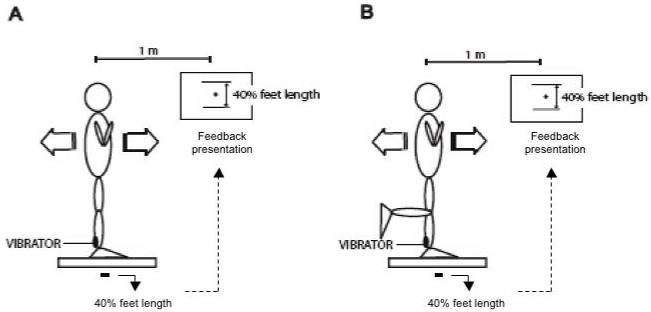
Schematic representation of the experimental set-up. Subjects were instructed to sway rhythmically while standing on both feet or on one foot (Panels A and B, respectively). Variations of these conditions included application of vibration to the Achilles tendon and closing the eyes. The nominal COP amplitude was 40% of the foot length, and the frequency was 0.5 Hz.

The instruction under all the conditions was to produce a continuous sway of the body in the AP direction in such a way that the displacement of the body’s COP was approximately 40% of the subject’s foot length. An auditory metronome paced the subject’s movements, and visual feedback on the AP location of the center of pressure (COP_AP) was provided by the monitor placed 1.0 m in front of the subject at the eye level. Subjects were asked to sway the body using mainly ankle rotation (“ankle strategy”, Horak and Nashner 1986; Alexandrov et al. 2001) and reach the most forward and backward point of the required distance at each metronome beat (Figure 2A and 2B); the metronome frequency was set at 1 Hz. Visual feedback was used only during the initial phase to promote similar peak-to-peak COP_AP displacement across the experimental conditions. The visual feedback was unavailable over the period of data recording.

A period of familiarization with the task was given to each subject prior to data collection. During the familiarization period, subjects performed the body sway for 3 minutes under each condition (except BV and UV) divided into 3 episodes of 60 s each. Since during the actual trials visual feedback was used only at the beginning of the trial, the subjects practiced to keep swaying while maintaining their pattern of COP displacement unchanged once the visual feedback was turned off. Vibration was not used during the familiarization period to avoid possible adaptation of its effects during the actual experiment. The sequence of conditions during the familiarization period was presented in a balanced order.

Each trial started with the subject standing upright quietly. Then, the metronome was turned on, and the subject was asked to begin swaying. Under the BO and UO conditions, data collection started after ten seconds of swaying and it lasted for 30 s. Under the other three conditions (BC, BV and, UV), data collection started 40 s after the initiation of sway. This was done to reach steady-state and avoid transient effects during either the eyes closed or vibration condition (Polonyova and Hlavacka 2001).

Only one trial was performed for each condition. From this single trial, twelve continuous sway cycles were taken for further analyzes (details in Data processing).The order of conditions was balanced across subjects (it was different for different subjects). Resting periods of two minutes were given between trials. A chair was placed behind the subject close to the force plate such that the subject could sit and take a rest without moving the feet.The average duration of the experiment was forty-five minutes, and none of the subjects complained of fatigue.

Data processing

All signals were processed off-line using LabView-5 and MatLab 6.5 software packages. Signals from the force platform were filtered with a 20 Hz low-pass, second order, zero-lag Butterworth filter, and COP_AP coordinate was computed using the following approximation:

$${\mathrm{COP}}_{\mathrm{AP}}=(-{\mathrm{M}}_{\mathrm{Y}}+({\mathrm{F}}_{\mathrm{X}}\ast \mathrm{h}))∕{\mathrm{F}}_{\mathrm{Z}},$$

where h is the distance between the force platform origin of coordinates and its top surface (h = 36 mm according to the manufacturer’s specifications)

For each experimental condition, twelve complete sway cycles recorded within a single trial were used for data analysis. The initiation (t₀) and end of each cycle (t₁) were defined by two consecutives extreme anterior positions of COP_AP. The duration of each cycle was time normalized such that the total duration of each cycle was always 100%. COP_AP coordinates within each 1% window were averaged resulting in a sequence of 100 points, each representing 1% of the sway cycle. COP_AP displacement was computed by subtracting the average COP_AP coordinate computed over the whole trial from the averaged COP_AP coordinate computed over each 1% window of the cycle.

EMG signals were first rectified and filtered with a 50 Hz low-pass, second-order, zero-lag Butterworth filter. Changes in muscle activation associated with COP_AP shift were quantified as follows. Rectified EMG signals were integrated over 1% time windows of each cycle (IEMG) as described in the previous paragraph. This procedure resulted in a sequence of 100 points for each muscles and each sway cycle.

In order to compare the IEMG indices across muscles and subjects, we normalized them by the EMG integrals computed for the control trials when the subjects stood and held the 5.0 Kg load. Within each of the two control trials, the rectified EMG signals were integrated over a time interval corresponding to the duration of 1% of the sway cycle as defined earlier. This time interval was selected in the middle of the control trials when all the muscles showed steady activation levels. IEMG indices for the dorsal muscles (SOL, GL, GM, BF, ST, ES) were divided by the EMG integrals computed for the control trial when the load was held quietly in front of the body. IEMG indices for the ventral muscles (TA, VM, VL, RF, RA) were divided by the EMG integrals computed for the control trial when the load was suspended behind the subject’s body. This method of normalization was used in earlier studies of muscle modes and synergies (Krishnamoorthy et al. 2003a,b; Wang et al. 2005; Danna-dos-Santos et al. 2007).

Statistics

Defining M-modes with principal component analysis (PCA)

For each subject and each experimental condition, the IEMG data formed a matrix with eleven columns corresponding to the eleven postural muscles and 1200 rows corresponding to 1% time windows of all twelve cycles analyzed. The correlation matrix among the IEMG was subjected to PCA (using SPSS software) with Varimax rotation. The factor analysis module with principal component extraction was employed. For each subject, the first five PCs were selected since PCs number six and higher did not have significantly loaded muscle activation indices in any of the conditions. Besides, analysis of the scree plots also showed that PCs number six and higher accounted for about the same amounts of the total variance across all the conditions.

We are going to address the first five PCs as muscle modes (M-modes, M₁, M₂, M₃, M₄, and M₅) and hypothesize that magnitudes of (gains at) the M-modes are manipulated by the controller to produce COP shifts. In other words, M-modes represent unitary vectors in the muscle activation space that can be recruited by the controller with different magnitudes.

The loadings at individual muscle activation indices were studied across the first five M-modes. In order to investigate qualitatively the structure of each M-mode, we analyzed how the loadings of IEMG indices of activation of the recorded postural muscles were organized within each M-mode and how they were distributed among the M-modes. We considered a muscle as part of a M-mode when its loading had an absolute value equal or larger than 0.50. We will refer to such cases as significant loadings (Krishnamoorthy et al. 2003a,b; Wang et al. 2005; Danna-dos-Santos et al. 2007).

Changes in the M-mode composition across conditions were studied using the number of occurrences of significant loadings in each M-mode. These were further studied with non-parametric methods. A Friedman’s test with the factors M-mode (M₁, M₂, M₃, M₄, and M₅) and Condition (BO, BC, BV, UO, and UV) was ran, and Mann-Whitney tests were used as post-hocs to explore significant effects. One-sample Wilcoxon’s tests were used as post-hocs in cases where no significant loadings were observed within a PC across all ten subjects; this happened in the BO and BC conditions.

Defining the Jacobian (J matrix) with multiple regression

Linear relations between changes in the magnitudes of M-modes (ΔM) and COP_AP shifts (ΔCOP_AP) were assumed and the corresponding multiple regression equations were computed over the 12 cycles performed by each subject and at each experimental condition. The coefficients in the regression equations were arranged in a Jacobian matrix (J):

$$\begin{array}{c}\Delta {\mathrm{COP}}_{\mathrm{AP}}={\mathrm{k}}_1\ast \Delta {\mathrm{M}}_1+{\mathrm{k}}_2\ast \Delta {\mathrm{M}}_2+{\mathrm{k}}_3\ast \Delta {\mathrm{M}}_3+{\mathrm{k}}_4\ast \Delta {\mathrm{M}}_4+{\mathrm{k}}_5\ast \Delta {\mathrm{M}}_5;\hfill \\ \mathbf{J}={\left[{\mathrm{k}}_1{\mathrm{k}}_2{\mathrm{k}}_3{\mathrm{k}}_4{\mathrm{k}}_5\right]}^{\mathbf{T}}\hfill \end{array}$$

Within this approach, the J matrices are reduced to (5×1) vector-columns. For each subject, this analysis was run over the twelve individual cycles for each time interval (each 1% of the total cycle). The analysis was run over full cycles (100 intervals per experimental condition).

UCM analysis: Computing the synergy index

The uncontrolled manifold (UCM) hypothesis assumes that the controller manipulates a set of elemental variables to stabilize a value or a time profile of a performance variable (Scholz and Schöner 1999; reviewed in Latash et al. 2002, 2007). In our analysis, gains at M-modes play the role of elemental variables, while COP_AP shift represents the performance variable. Hence, we analyze the variance in the M-mode space at each phase of the sway cycle and compare its two components. One component of the M-mode variance is compatible with a stable, i.e. reproducible from cycle to cycle, value of the COP_AP coordinate (estimated as its average value at that phase of the cycle). The other variance component led to changes in the COP_AP coordinate. To compute the two variance components, the following analysis was performed.

For each cycle (n), IEMG indices were computed and transformed into ΔM using the results of the PCA in Step-1 of the analysis. Further, two types of analysis were run. The first analysis used only the first three M-modes that satisfied the acceptance criteria under each of the five conditions. Under the three most challenging conditions (BV, UO, and UV), M₄ and M₅ were accepted as well. Hence, under those conditions the analysis was repeated for the complete set of five M-modes.

Hence, the ΔM space had the dimensionality of either n=3 or n=5. A hypothesis that a particular magnitude of ΔCOP_AP is stabilized by co-variation of ΔM magnitudes accounts for one degree of freedom (d=1). Thus, the system is redundant with respect to the task of stabilizing particular ΔCOP_AP values. The mean magnitudes of each ΔM were computed for each subject and each task separately across samples over a trial. Since the model relating ΔM to ΔCOP_AP is linear, the ΔM mean values were subtracted from each ΔM computed value and the residuals were subjected to further analysis as follows.

The UCM represents combinations of M-mode magnitudes that are consistent with a stable (reproducible from cycle to cycle) value of ΔCOP_AP. The UCM was calculated as the null-space of the corresponding J matrix (defined at Step-2 of the analysis). The null-space of J is a set of all vector solutions x of a system of equations Jx=0. This space is spanned by basis vectors, ε_i. The vector of individual mean-free Ms was resolved into its projection onto the null-space:

$$f_{\mathit{UCM}}=\sum _{i=1}^{n-d}({\underset{‒}{\epsilon }}_i^T\cdot \left(\Delta \mathbf{M}\right)){\underset{‒}{\epsilon }}_i$$

and component orthogonal to the null-space:

$$f_{\mathit{ORT}}=\left(\Delta \mathbf{M}\right)-f_{\mathit{UCM}}$$

The amount of variance per DOF within the UCM is:

$$V_{\mathit{UCM}}={\sigma }_{\mathit{UCM}}^2=\sum _{i=1}^N{f}_{\mathit{UCM}}^2∕\left((n-d)N_{\text{trials}}\right)$$

and orthogonal to the UCM is:

$$V_{\mathit{ORT}}={\sigma }_{\mathit{ORT}}^2=\sum _{i=1}^N{f}_{\mathit{ORT}}^2∕\left(d{N}_{\text{trials}}\right)$$

V_UCM and V_ORT were the main dependent variables used in this analysis. In lay terms, they correspond to “good variability” (V_UCM that does not affect ΔCOP_AP computed for a certain time interval during the oscillation cycle) and “bad variability” (V_ORT that changes ΔCOP_AP). Two-way mixed design ANOVA with the factors Condition (BO, BC, BV, UO, and UV) and Variance-Component (V_UCM and V_ORT) was performed to analyze the effects of experimental conditions on the two variance components.

To quantify the relative amount of the total variance that is compatible with stabilization of a particular COP_AP shift we used an index (ΔV) reflecting the difference between the variance within the UCM and orthogonal to the UCM. ΔV was computed as:

$$\Delta \mathrm{V}=(V_{\mathit{UCM}}-V_{\mathit{ORT}})∕V_{\mathit{TOT}}$$

where all variance indices are computed per degree of freedom; V_TOT stands for total variance. A one-way ANOVA with the factor Condition (BO, BC, BV, UO and UV) was used to test the effect of condition on ΔV when only the first three M-modes were considered. A two-way mixed design ANOVA with factors Condition (BV, UO and UV) and Dimensionality (n=3; n=5) was used to test the effect of condition and the use of either three or five M-mode sets during the data processing on ΔV.

Results

This section is organized in the following way. First, the basic patterns of COP_AP shifts and muscle activity are described. Further, the results of the PCA are presented, and M-modes are identified and analyzed. Finally, we describe the results of the UCM analysis applied to the M-mode data.

Patterns of COP_AP and muscle activity

Across all five conditions of body sway, the subjects were able to show qualitatively similar, sine-like time profiles of COP_AP. The average COP_AP displacements across the ten subjects are shown in Figure 3A (dark bars); they were 38.47 ± 1.30%, 46.99 ± 2.39%, 44.43 ± 2.17%, 41.10 ± 1.60%, and 39.70 ± 1.78% of foot length for the BO, BC, BV, UO, and UV conditions, respectively. To remind, the nominal target amplitude was 40% of the foot length. Figure 4 shows the COP_AP profile averaged across 12 cycles during body sway performed by a typical subject under all five experimental conditions. Note the similarity of the shapes across all five conditions. Figure 3A (dark bars) also presents the average mean velocity of COP_AP shift and its average frequency of oscillation across the ten subjects. The average mean velocity of COP_AP was 9.90 ± 0.45 cm/s, 12.07 ± 0.64 cm/s, 11.45 ± 0.58 cm/s, 10.96 ± 0.37 cm/s, and 10.62 ± 0.44 cm/s for the BO, BC, BV, UO, and UV conditions respectively. The average frequency of COP_AP was 0.50 ± 0.00 Hz, 0.50 ± 0.00 Hz, 0.49 ± 0.07 Hz, 0.50 ± 0.00 Hz, and 0.49 ± 0.00 Hz for the BO, BC, BV, UO, and UV conditions respectively (Figure 3B).

Figure 3.

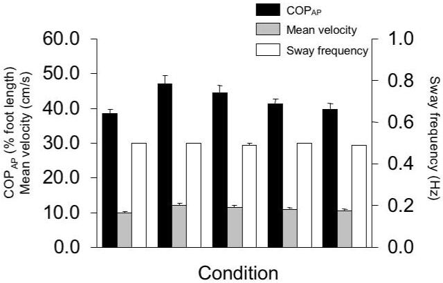
Means and standard errors (across subjects) of peak-to-peak COP_AP in % of foot length (Panel A, dark bars), mean velocity (Panel A, light bars), and frequency of body oscillation (Panel B) for the five different experimental conditions are shown. BO - bipedal stance with eyes open, BC - bipedal stance with eyes closed, BV - bipedal stance with eyes closed and vibration applied bilaterally to the Achilles tendons, UO - unipedal stance with eyes open (no vibration), UV - unipedal vibration with eyes open and vibration applied unilaterally to the Achilles tendon.

Figure 4.

Average COP_AP displacement across 12 cycles for a representative subject (subject 2). Different lines represent COP_AP patterns under the five experimental conditions. Note the similarity in the time profiles and similar sway amplitudes in the five tasks.

Effects of the five different experimental conditions on peak-to-peak COP_AP displacement, mean velocity, and oscillation frequency were tested with three one-way repeated measures ANOVAs with the factor Condition (BO, BC, BV, UO, and UV). ANOVA confirmed significant effect of Condition on peak-to-peak COP_AP displacement (F_{[4, 36]} = 5.63, p<0.01) and on the mean velocity of COP_AP (F_{[4, 36]} = 5.45, p<0.01). The pair-wise comparisons showed significant differences only between the BO and BC conditions (p<0.05). There were no significant effects of Condition on frequency of oscillation (F_{[4, 36]} = 1.06, p>0.05). Altogether, these results indicate that the subjects were able to keep the pace and COP_AP trajectories similar across the conditions.

There were regularities in the patterns of activation of the leg and trunk muscles across all five experimental conditions of sway. In particular, during the forward-to-backward part of the sway cycle (0 to 50%), there was a decrease in the level of activation of dorsal muscles (SOL, GL, GM, BF, ST, and ES) and an increase in the activity of ventral muscles (TA, VM, VL, RF, and RA). At the instant of the most backward COP location (50% of the cycle time), ventral muscle activity was typically high and the dorsal muscle activity was low. Over the backward-to-forward sway (51 to 100%), the ventral muscles activity decreased while the dorsal muscles exhibited an increase in their activity. This overall pattern is illustrated in Figure 5 that shows EMG profiles for ten postural muscles in a representative subject during body sway under BO (thick lines) and UV(dashed lines). Note that some muscles (SOL, GM, GL, ST, TA, RF, and VM) showed an increase in the peak EMG levels and also a shift from the smooth, sine-like changes in the muscle activity (at BO) to more abrupt bursts under the UV condition. However, other muscles (BF, ES, and VL) did not show any visible increase in the level of activity under more challenging conditions such as UV.

Figure 5.

Integrated over each 1% of the cycle and normalized muscle activation indices (IEMG) averaged across 12 cycles for a typical subject under the BO (bipedal stance, open eyes) and UO (unipedal stance, open eyes) conditions (solid and dashed lines, respectively). Panels A-F show IEMG of dorsal muscles (SOL, GM, GL, BF, ST, ES) and panels G-J show IEMG of ventral muscles (TA, VL, RF, VM, RA). IEMG is in arbitrary units, and sway cycle is percent of its total duration. Phases 0% and 100% indicate the most anterior COP position (‘Front’) and phase 50% indicates its most posterior position (‘Back’). The scales have been selected for better visualization.

Principal component analysis (PCA)

To identify groups of muscles whose activity was modulated in parallel during the sway, we used PCA (as described in the Methods). PCA was run on data combined over the whole cycle duration and over the 12 sway cycles, i.e. on the 1200×11 IEMG matrix. Based on the criteria described in the Methods, the first five PCs were chosen in each data set. The five first PCs were selected since under the BV, UO, and UV conditions, each of the first five PCs could contain significantly loaded muscle activation indexes. Across all conditions, PC6 through PC11 showed no significant loadings. Under the BO and BC conditions, virtually all significant loading were in the first three PCs with a few (for the total of six cases across all subjects) in PC4 and none in PC5.

The first five principal components (which we refer to as muscle modes, M₁, M₂, M₃, M₄, and M₅) accounted, on average, for 98.41% (± 0.18%) of the total variance during body sway performed under the BO condition, 98.64% (± 0.13%) under the BC condition, 97.82% (± 0.24%) under the BV condition, 96.07% (± 0.68) under the UO condition, and 95.39% (± 0.84%) under the UV condition. Figure 6A illustrates the total amount of variance explained by the first five M-modes averaged across subjects under each experimental condition. Note that there is a drop in the variance explained from BO and BC through UV. This drop was significant according to a one-way ANOVA with the factor Conditions (BO, BC, BV, UO, and UV) on the z-scores of the amount of variance explained by the first five M-modes (F_{[4, 45]}=12.08, p<0.001). Tukey’s pair-wise contrasts showed significant differences between the following comparisons: BC vs. UO and UV (p<0.001); BO vs. UO and UV (p<0.01); and BV vs. UV (p<0.05). However, we would like to emphasize that the total amount of explained variance was high across all conditions reaching values always over 90%.

Figure 6.

Panel A: Averaged across subjects amounts of variance explained by the five first principal components (M-Modes). Note the drop in the amount of variance from BC through UV conditions. Panel B: Averaged across subjects amounts of variance explained by each M-mode (M₁ through M₅). Note that there is a drop in the variance explained by the first two M-modes and an increase of the variance explained by the last three M-modes across the five conditions.

The amount of variance accounted for by each M-mode varied across the experimental conditions. Specifically, the first two M-modes (M₁ and M₂) showed a drop in the amount of variance from the relatively easy conditions (BO and BC) to the more challenging conditions (BV, UO, and UV), while the remaining three M-modes showed an opposite trend (Figure 6B). This finding is illustrated in Figure 6B were the average amount of variance explained by each M-mode across the ten subjects is shown. Note that both black and gray bars (M₁ and M₂, respectively) show a drop in their values from BO through UV while the striped, checkered and white bars representing M₃, M₄, and M₅ show an increase in their values. The average amount of variance explained by M₁ and M₂ combined (ΣVar(M₁,M₂)) was 81.37 ± 1.77%, 81.64 ± 2.08%, 68.61 ± 1.72%, 66.94 ± 3.47%, and 64.27 ± 2.66% for the BO, BC, BV, UO, and UV conditions, respectively. For the same conditions, the average amount of variance explained by the remaining 3 M-modes (ΣVar(M₃,M₄,M₅)) was 17.11 ± 1.68%, 17.00 ± 1.98%, 29.20 ± 1.64%, 29.13 ± 2.89%, and 31.12 ± 2.04% . This trend was confirmed by a two-way mixed-design ANOVA with factors Condition (BO, BC, BV, UO, and UV), and Variance (ΣVar(M₁,M₂); ΣVar(M₃,M₄,M₅)). There was a significant Conditio × Variance interaction (F_{[4, 90]} = 19.74, p<0.001) in addition to significant main effects of Condition (F_{[4, 90]} = 3.73, p<0.01) and Variance (F_{[1, 90]} = 697.41, p<0.001). The effect of Variance confirmed that ΣVar(M₁,M₂) was higher than ΣVar(M₃,M₄,M₅) across all conditions. The effects of Condition, reflected a significant difference between BC and UV (Tukey’s pair-wise comparisons, p<0.05). Condition × Variance interaction reflected a siginificant difference between changes in ΣVar(M₁,M₂) and ΣVar(M₃,M₄,M₅) between each of the two easier conditions (BO and BC) and each of the three more challenging conditions (BV, UO and UV) confirmed by Tukey’s pair-wise comparisons (p < 0.05).

The composition of individual M-modes was similar across subjects and between the BO and BC conditions; however, under the BV, UO, and UV conditions this composition showed modifications. In general, under the BO and BC conditions, subjects showed significant loadings of the muscle activation indices mainly concentrated in the first two M-modes. The third M-mode rarely had more than one significantly loaded muscle index. Commonly, significant loadings of the indices for the dorsal muscles (SOL, GM, GL, BF, ST, and ES) were united in one of the first two M-modes, while the indices for the ventral muscles (TA, VL, VM, and RF) were united in the other of the two first M-modes. Sometimes, indices for most muscles, dorsal and ventral, were found in the same M-mode (M₁), but in such cases the loading coefficients for the dorsal and ventral muscles always had opposite signs.

Substantial modifications of the M-mode composition were found under the BV, UO, and UV conditions. In particular, we observed a tendency of the significant loadings to emerge in the third, fourth, and fifth M-mode (M₃, M₄, and M₅).

Table 1 shows individual loadings for all muscles under the BO and UV conditions for a typical subject. Note that under the BO condition, two distinct subgroups of significant loadings can be seen in the first M-mode (significant loading values are shown with bold numbers). The first subgroup contains indices for all six dorsal muscles with positive loading factors while the second subgroup contains indices for four ventral muscles with negative loading values. M₂ shows one significant loading for a dorsal muscle (SOL) and four significant loadings of the opposite sign for the ventral muscles (TA, VL, RF, and VM). Under the UV condition, significant loadings were seen in M₃ (for BF and ST), M₄ (for RA), and M₅ (ES).

Table 1.

Loading coefficients for the PCA

	BO						BV
	PC1	PC2	PC3	PC4	PC5		PC1	PC2	PC3	PC4	PC5
SOL	0.85	-0.50	0.07	-0.06	-0.01	SOL	0.54	-0.77	-0.28	0.17	-0.01
GM	0.87	-0.46	0.13	0.00	-0.03	GM	0.60	-0.67	-0.37	0.17	-0.04
GL	0.90	-0.38	0.03	-0.13	-0.05	GL	0.39	-0.82	-0.34	0.20	0.01
BF	0.86	-0.42	0.18	0.12	0.09	BF	0.61	-0.49	-0.54	0.23	-0.14
ST	0.85	-0.45	0.18	0.00	0.04	ST	0.73	-0.51	-0.35	0.20	-0.20
ES	0.95	0.10	0.15	0.02	0.26	ES	0.06	-0.28	-0.95	0.01	0.01
TA	-0.61	0.71	-0.05	0.31	0.02	TA	-0.92	0.32	0.00	-0.06	0.13
VL	-0.58	0.77	-0.03	-0.17	0.08	VL	-0.91	0.31	0.14	-0.15	-0.13
RF	-0.60	0.79	-0.06	0.01	0.00	RF	-0.91	0.33	0.14	-0.18	-0.01
VM	-0.56	0.81	-0.03	0.03	0.00	VM	-0.92	0.27	0.13	-0.22	0.01
RA	0.05	-0.18	0.95	-0.02	-0.26	RA	-0.20	0.18	0.05	-0.96	0.01
	UO						UV
	PC1	PC2	PC3	PC4	PC5		PC1	PC2	PC3	PC4	PC5
SOL	-0.61	0.49	0.34	-0.50	0.06	SOL	0.85	-0.48	0.09	0.12	0.13
GM	-0.67	0.38	0.22	-0.57	0.08	GM	0.80	-0.54	0.13	0.10	0.10
GL	-0.57	0.53	0.36	-0.47	0.02	GL	0.85	-0.45	0.09	0.13	0.20
BF	-0.40	0.71	0.11	-0.53	0.06	BF	0.76	-0.27	0.51	0.17	0.13
ST	-0.18	0.98	-0.03	-0.09	-0.05	ST	0.22	0.04	0.95	0.08	-0.17
ES	0.32	0.02	-0.93	0.11	0.03	ES	-0.39	0.38	0.37	0.09	-0.74
TA	0.60	-0.34	-0.48	0.38	-0.11	TA	-0.71	0.52	-0.20	-0.06	-0.26
VL	0.94	-0.23	-0.14	0.10	-0.13	VL	-0.37	0.91	0.00	-0.04	-0.14
RF	0.91	-0.17	-0.29	0.21	-0.07	RF	-0.42	0.88	0.01	-0.07	-0.19
VM	0.88	-0.22	-0.29	0.25	-0.09	VM	-0.44	0.87	0.03	-0.09	-0.13
RA	0.13	0.02	0.01	0.04	-0.99	RA	0.15	-0.08	0.09	0.98	-0.04

Data for a typical subject under the BO (bipedal stance with eyes open), BV (bipedal stance with eyes open and vibration applied bilaterally to the Achilles tendon), UO (unipedal stance with eyes open), and UV (unipedal stance with eyes open and vibration applied unilaterally to the Achilles tendon) conditions are shown. Loadings with the absolute values over 0.5 are shown in bold. SOL - soleus, GM - medial gastrocnemius, GL - lateral gastrocnemius, BF - biceps femoris, ST - semitendinosus, ES - erector spinae, TA - tibialis anterior, VL - vastus lateralis, VM - vastus medialis, RF - rectus femoris, RA - rectus abdominis.

The data summarizing the total number of significant loadings observed in each M-mode for all ten subjects are shown in Figure 7. Note that, as compared to the BO and BC conditions, there is a decrease in the total number of significant loadings within M₁ and M₂ under the BV, UO, and UV conditions (black and gray bars, respectively) and a parallel increase in the number of significant loadings in M₄ and M₅ (white and checkered bars). This finding was confirmed by a series of non-parametric statistic tests. First, a Friedman’s test performed with factors M-mode (M₁, M₂, M₃, M₄, and M₅) and Condition (BO, BC, BV, UO, and UV) showed overall significance (χ²_[4]= 18.68, p<0.01). Kruskal-Wallis tests ran as post-hocs confirmed a significant effect of M-mode but not of Condition. Mann-Whitney tests showed significant differences for the following comparisons: M₁ vs. all other M-modes (p<0.01 for all comparisons), M₂ vs. all other M-modes (p<0.01 for all comparisons), M₃ vs. M₄ and M₅ (p<0.05), and M₄ vs. M₅ (p<0.05).

Figure 7.

The total number of significant loadings of the indices of muscle activation for each M-mode for all ten subjects under each experimental condition. Note a decrease in the number of significant loadings in the M₁- and M₂- modes from BC through UV conditions and a parallel increase in the number of significant loadings for the M₃- M₄-, and M₅-modes.

To analyze possible interactions between the factors M-mode (M₁, M₂, M₃, M₄, and M₅) and Condition (BO, BC, BV, UO, and UV) on the number of significant loadings observed, another series of Mann-Whitney tests were ran. For M₁, M₂, M₄, and M₅ the tests showed that the BO and BC conditions were significantly different from the BV, UO, and UV conditions (p<0.05 for all comparisons). For M₃, the BC condition was significantly different from the BV, UO, and UV conditions (p<0.05 for all comparisons). So, taken together these results suggest that under more challenging conditions, more significantly loaded muscle indices appeared in M₄ and M₅

UCM analysis

Data from twelve continuous sway cycles for each of the five experimental conditions were used to perform analysis of the structure of variability in the space of M-modes. The method partitions the total variance in the M-mode space across cycles into two components. The first component (V_UCM) is within an uncontrolled manifold (UCM) approximated as the null-space of the corresponding J matrix describing the linear relations between changes in the magnitude of M-modes (ΔM) and COP_AP shifts (ΔCOP_AP) (see Methods). The other component (V_ORT) is within a sub-space orthogonal to the UCM. Further, we computed an index (ΔV) reflecting the normalized difference between V_UCM and V_ORT. We interpret positive values of ΔV as reflecting a multi-M-mode synergy stabilizing the average COP shift.

Using the same data sets we performed two separated analyzes that differed in the number of accepted M-modes. First, we analyzed the variability in the 3-dimensional space of the first 3 M-modes across all five conditions. In the second analysis, we considered the 5-dimensional space of the first five M-modes (dimensionality n= 5). For this second analysis, only the data for the three most challenging experimental conditions were considered (BV, UO, and UV). We did not perform this analysis for the BO and BC conditions, because modes M₄ and M₅ accounted for little variance and had no significantly loaded muscle indices in those conditions.

The J matrix was computed using multiple linear regression of changes in the magnitudes of M-modes (ΔM) against COP_AP shifts (ΔCOP_AP) over the 12 cycles performed by each subject, for each experimental condition separately. The coefficients in the regression equations were arranged in a vector matrix (J matrix) and it null-space was used to approximate the uncontrolled manifold. In cases where we accepted only the first three M-modes for further analysis, the J matrix was a 3×1 vector-column. In cases where the five first M-modes were accepted, the J matrix was a 5×1 vector column.

Figure 8 shows the average across the ten subjects amount of variance in ΔCOP_AP explained by the regression model (with standard errors). The average amount of variance explained based on the first 3 M-modes was 50.55 ± 2.93%, 49.82 ± 2.60%, 47.25 ± 3.49%, 43.57 ± 3.03%, and 40.03 ± 4.08% for the BO, BC, BV, UO, and UV conditions, respectively. For the same conditions, the average amount of variance explained based on the first 5 M-modes was 53.26 ± 3.01%, 54.59 ± 2.61%, 49.75 ± 3.04%, 45.43 ± 3.03%, and 41.92 ± 3.85%. Note that there was a decrease in the amount of variance explained by the linear model from less challenging conditions through the more challenge ones (BO through UV). A two-way mixed design ANOVA with factors Condition (BO, BC, BV, UO and UV) and Dimensionality (n=3; n=5) was run on the z-scores of the variance accounted for by the linear model. There was only a significant effect of Condition (F_[4,90]=4.16, p<0.01). Tukey’s tests confirmed a significant difference between BO and UV, and between BC and UV.

Figure 8.

Variance explained by linear regression of ΔCOP_AP against changes in the three M-mode (black bars) and in the five M-mode magnitudes (white bars). Note the drop in the amount of variance explained from BO through UV.

In the three-M-mode analysis, there was an increase of V_UCM from BO through BV conditions; the averaged across subjects V_UCM values were similar for the UO and UV conditions but higher than those computed for the BO, BC, and BV conditions. These results are displayed in Figure 9A, which shows the V_UCM and V_ORT indices per degree-of-freedom averaged across all ten subjects. Note that V_UCM (black bars) was consistently larger than V_ORT.

Figure 9.

Panels A and B: Averaged across subjects V_UCM and V_ORT components of the total variance for each condition (with standard error bars) when 3 or 5 M-modes were considered. Dark bars represents V_UCM while light bars represent V_ORT. Panels C and D: Means and standard errors for ΔV across subjects when 3 or 5 M-modes were considered. Note that the values are positive and show inconsistent changes with the task. Panels E and F: Time profiles of ΔV averaged across subjects over the full sway cycle under all five experimental conditions of body sway when 3 or 5 M-modes were considered.

To analyze the effects of the experimental conditions on the two variance components for the three-M-mode analysis, a two-way mixed-design ANOVA with the factors Condition (BO, BC, BV, UO, and UV) and Variance-Component (V_UCM and V_ORT) was performed. There were significant main effects of both Condition (F_{[4, 90]}= 6.44, p<0.001) and Variance-Component (F_{[1, 90]}= 15.20, p<0.001) without a significant interaction (p>0.1). The effect of Variance-Component confirmed that V_UCM > V_ORT. Tukey’s pair-wise comparisons showed significant differences between the following pairs: BO and UO (p<0.001), BO and UV (p<0.01), BC and UO (p<0.01), BC and UV (p<0.01), BV and UO (p<0.01), BV and UV (p<0.01). All other pair-wise comparisons did not reach significance.

The five-M-mode analysis also showed lower V_UCM values in the BV condition as compared to the UO and UV conditions that were not different from each other (Figure 9B). This analysis confirmed significantly higher V_UCM values as compared to V_ORT. Two-way mixed-design ANOVA with the factors Condition (BV, UO, and UV) and Variance-Component (V_UCM and V_ORT) showed significant main effects of both Condition (F_{[2, 54]}= 3.48, p<0.05) and Variance-Component (F_{[1, 54]}= 15.86, p<0.001) without a significant interaction (p>0.1). The effect of Variance-Component confirmed that V_UCM > V_ORT. Tukey’s pair-wise comparisons showed significant differences between BV and UO conditions (p<0.05). All other pair-wise comparisons did not reach significance.

To test whether the two variance components changed similarly across the experimental condition, an index (ΔV) reflecting their normalized difference was used. The dependence of the average magnitude of ΔV on the experimental conditions is illustrated in Figures 9C and 9D. The ΔV index was always significantly larger than zero for all conditions and for both three-M-mode and five-M-mode analyses, which means that most variance within the M-mode space was within the UCM.

A one-way ANOVA with the factor Condition (BO, BC, BV, UO and UV) was used to test the effect of condition on ΔV when only the first three M-modes were considered. This ANOVA showed no effect of Condition (F_[4,45] = 0.68, p>0.5). A two-way mixed design ANOVA with factors Condition (BV, UO and UV) and Dimensionality (n=3; n=5) was used to test the effect of condition and the type of analysis (three or five M-modes) on ΔV. This two-way ANOVA shows significant main effect for Condition (F_[2,54] = 3.30, p<0.05) but no effect of Dimesionality (F_[1,54] = 0.70, p>0.5) and no interaction (p>0.1). Tukey’s pair-wise comparisons showed significant differences between the BV condition as compared to the UO and UV conditions (p<0.05). All other pair-wise comparisons did not reach significance.

Time changes of the ΔV index for all five conditions are shown in panels E and F of Figure 9. No clear pattern of ΔV modulation within the sway cycle was found.

Discussion

The results of the study provide support for the first hypothesis that the composition of M-modes could adjust under challenging conditions. However, the results speak against the second hypothesis that the index of M-mode co-variation would become weaker in more challenging conditions. In particular, in accordance with the first hypothesis, more challenging postural tasks were associated with an increase in the number of principal components (M-modes) that contained significantly loaded indices of muscle activation. However, the performance of more challenging tasks was not associated with a decrease in the index of the multi-M-mode synergy stabilizing COP shifts. The introduced index of the synergy was comparable across all conditions, and there was no modulation of this index over the sway cycle. Further in the Discussion, we analyze the findings with respect to the hierarchical organization of muscle groups in tasks that require keeping vertical posture.

Muscle modes in the hierarchy of postural control

At virtually any level of description, human bodies have more elements than necessary to perform typical motor tasks. Bernstein was arguably the first to make the redundancy of the neuromuscular system a central issue of motor control (Bernstein 1967). He suggested that the central nervous system united elements into groups (synergies) and used a fewer number of control variables partly solving the problem of motor redundancy.

A recent development of these ideas combined with the principle of abundance (Gelfand and Latash 1998) has allowed to introduce a definition of synergies that made possible their quantitative analysis (reviewed in Latash et al. 2002, 2007). At any level of a control hierarchy, synergies have been defined as neural organizations of elements that ensure low variability (high stability) of a particular overall output variable of that level. For example, in multi-digit studies, two levels of control have been identified. At the upper level, the task is distributed between the actions of the thumb and the virtual finger (VF, an imagined finger with the mechanical action equal to combined action of the four fingers, Arbib et al. 1985; Mackenzie and Iberall 1994). At the lower level, the action of VF is distributed among the actual fingers of the hand. Synergies stabilizing the overall mechanical action of the hand at the thumb-VF level and those stabilizing the VF action at the individual finger level have been described (reviewed in Zatsiorsky and Latash 2004).

The two-level hierarchical scheme of postural control mentioned in the Introduction may be viewed as similar to that of the hierarchical control of the hand. One may view M-modes as “virtual muscles” manipulated at the higher level of the control hierarchy, while mapping of M-modes on actual muscle activation is analogous to mapping of the VF action on individual finger actions. The only difference is that there are always two digits considered at the higher level of the hierarchy in hand studies, the thumb and VF, while the number of “virtual muscles” can vary at least between three and five as shown in our current study.

Recently, the idea that the neural controller unites muscles into groups to reduce the number of control variables (Hughlings Jackson 1889) has led to the emergence of a variety of methods identifying such muscle groups during whole-body tasks such as postural preparation and responses to perturbations, stepping, and swaying (Krishnamoorthy et al. 2003a,b; Ivanenko et al. 2004, 2005; Ting and Macpherson 2005; Torres-Oviedo et al. 2006; Torres-Oviedo and Ting 2007). Many of these studies used matrix factorization techniques to identify eigenvectors in the space of muscle activations including the principal component analysis with factor extraction (for comparison of different methods see Tresch et al. 2006). Such eigenvectors have been termed synergies or muscle modes (M-modes).

The term ‘muscles mode’ (or M-mode) was introduced to imply that such muscle groups play the role of elemental variables to construct synergies for the purpose of ensuring low variability (high stability) of important performance variables (Krishnamoorthy et al. 2003a,b). However, as mentioned in the Introduction, addressing a variable as a performance variable stabilized by a synergy or as an elemental variable depends on the level of analysis. For example, muscle activation level may be viewed as a performance variable stabilized by co-varied activity of motor units or as an elemental variable forming a multi-muscle synergy. Hence, in this study we accepted, as an axiom, that the control of whole-body movements is based on an at least two-level hierarchy. At the lower level, M-modes are formed by synergies in the space of individual muscle activations while at the higher level M-modes play the role of elemental variable and form synergies stabilizing physical variables important for the interaction with the environment.

This hypothesis implies, in particular, that M-mode composition may change under certain changes in external conditions of task execution. A few studies have indeed described atypical co-contraction M-modes when subjects performed whole-body tasks while standing on a board with a reduced support area (Krishnamoorthy et al. 2004b; Asaka et al. 2007).

In the current study, we used relatively minor complicating factors for the postural tasks. For example, closing eyes is known to increase postural sway (Allum and Pfaltz 1985; Fitzpatrick et al. 1992; Schumann et al. 1995) but it is not associated with losing balance in most persons. Standing on one foot is a more challenging task, (Tropp and Odenrick 1988; Goldie et al. 1992; Harrison et al. 1994), but most people can do it easily. Vibration applied to the Achilles tendons is known to produce major destabilizing effects on vertical posture during quiet standing (Lackner and Levine 1979; Nakagawa et al 1993; Calvin-Figuiere et al. 1999), likely because of the unusually high level of activity of primary muscle spindles (Lackner and Levine 1979). It is also known to lead to reorganization of postural adjustments to self-triggered perturbations (Kasai et al. 2002; Slijper and Latash 2004) and to produce significant changes in locomotor patterns (Ivanenko et al 2000). Note, however, that even in the most challenging condition of our study - swaying while standing on one foot with vibration of the Achilles tendon - the subjects were able to perform the task successfully without losing balance. This is in contrast to the frequent losses of balance reported in the mentioned studies by Krishnamoorthy, Asaka and their colleagues who used more challenging tasks performed while standing on a narrow support surface (Krishnamoorthy et al. 2004; Asaka et al. 2007).

While the two least challenging conditions (swaying with the eyes open and closed) were associated with three M-modes (similar to earlier studies, Krishnamoorthy et al. 2003a,b, Wang et al. 2005, Danna-Dos-Santos et al. 2007), the three more challenging ones were associated with the emergence of the fourth and fifth M-modes that showed significant loadings of muscles that used to be significantly loaded in one of the first three M-modes under the BO and BC conditions. Was this a split of one M-mode into two or a more complex reorganization? We cannot answer this question, partly because of the relatively arbitrary identification of significantly loaded muscle activations as those with the loading factors over 0.5. However, overall, the increase in the number of M-modes may be interpreted as an increase in the number of control variables manipulated by the controller at the higher level of the hierarchy as the tasks became more complex.

There was substantial variability across the subjects in the composition of the fourth and fifth M-modes; more frequently these M-modes contained significantly loaded indexes of activation for dorsal proximal muscles such as BF, ST, and ES (see Table 1). These observations fit the hypothesis on different roles of the distal and proximal muscles in anticipatory postural adjustments during challenging postural tasks (Shiratori and Latash 2000). They are also compatible with the reports on muscle groupings seen during balance recovery following an external perturbation that resemble the hip strategy of postural stabilization (Torres-Oviedo et al. 2006; Torres-Oviedo and Ting 2007).

The observed adjustments in the composition and number of M-modes corroborate the idea that M-modes represent not hard-wired muscle groupings but flexible combinations of muscle activations. On the other hand, several earlier studies have shown similarity of the M-mode composition across subjects and tasks when whole-body tasks were performed in natural standing conditions without any complicating factors (Krishnamoorthy et al. 2003b; Danna-Dos-Santos 2007). This combination of low variability and flexibility of the M-mode composition is a trademark of a synergy (Latash et al. 2007) supporting the hypothesis that M-modes represent synergies at the lower level of the assumed control hierarchy.

Reduction of motor variability and flexible motor patterns

Within our approach, synergies are viewed as neural organizations of elemental variables with the purpose to stabilize a performance variable (reviewed in Latash et al. 2007). This definition implies that the main purpose of a synergy is to decrease variability of the corresponding performance variable. Recent studies, however, have emphasized another important feature of synergies, namely that they allow the central nervous system to be flexible in performing motor tasks such that secondary tasks could be performed using the same set of elemental variables, without sacrificing accuracy of performing the primary task (Gorniak et al. 2008; Zhang et al. 2008). For example, a multi-joint synergy involved in carrying a cup of coffee allows to open the door with the elbow of the same arm without spilling the contents of the cup.

In postural studies, several performance variables could be stabilized by co-varied involvement of the same set of M-modes. In particular, COP trajectories in the anterior-posterior and in the medio-lateral direction could be stabilized simultaneously in preparation to stepping (Wang et al. 2005), while COP trajectory in the anterior-posterior direction and the shear force in the same direction could be stabilized simultaneously during an unusual task of producing a large shear force pulse (Robert et al. 2008). A priori, we hypothesized that an increase in the number of M-modes could make the task more challenging for the controller and would have adverse effects on its ability to form COP-stabilizing synergies. This prediction, however, has been falsified in the experiments (see Figure 8). With the benefit of a hindsight, this outcome makes sense. It fits the general view on motor redundancy as not a complicating factor for the controller but as a luxury that allows to ensure stable behaviors with respect to various performance variables and in various conditions (Latash et al. 2007; Zhang et al. 2008). Hence, adding elements at any level of a hierarchy is not expected to make control more complex, rather to make it more powerful.

In our study, the larger sets of M-modes could have allowed the same muscles to be used to stabilize not only the explicitly required variable (COP coordinate in the anterior-posterior direction) but also other variables that may be viewed as reflecting secondary tasks. For example, during swaying while standing on one leg, COP coordinate in the medio-lateral direction had to be kept within a relatively narrow range corresponding to the decreased support area. When tendon vibration was applied, the distorted sensory information from the calf muscles (Lackner and Levine 1979) could force the central nervous system to attend to other sources of sensory information (for example, from proximal leg muscles, as suggested by studies of patients with diabetes, Van Deursen and Simoneau 1999) and stabilize corresponding mechanical variables. Having a larger set of M-modes allowed the controller to attend to those secondary components of the task without a detrimental effect on the index of stabilization (ΔV, see Figure 9) of the performance variable related to the explicit, primary task component (COP coordinate in a sagittal plane).

Potential role of sensory and biomechanical factors

We manipulated both sensory signals and mechanical conditions for the main task of body sway. In particular, closing the eyes may be viewed as a purely sensory manipulation. Vibrating the Achilles tendons has a strong sensory effect, particularly mediated by the primary endings of the muscle spindles (Brown et al. 1967), but it can also lead to the tonic vibration reflex (Eklund and Hagbarth 1966), which may affect the mechanics of the movement. Performing the task while standing on one foot may be viewed as mechanically more challenging because of the smaller size of the support area in the medio-lateral direction. In unipedal conditions, however, there are also changes in the sensory information coming from both legs, the unloaded one and the double-loaded one.

Earlier studies have reported modifications in the composition of muscle modes in response to changes in both biomechanical (Krishnamoorthy et al. 2004) and sensory factors (Cheung et al. 2005; M-modes have beeed addressed as synergies in that study). In our study both, primarily sensory (vibration) and primarily mechanical (unipedal stance), factors had comparable effects on the M-mode composition.

There have also been reports of task-specific changes in the muscle groupings, for example during forward and backward pedalling (Raasch and Zajac 1999; Ting et al. 1999). In this study, we did not modify the explicit task. However, earlier studies used a variety of tasks such as quick arm motion, load release, stepping, and voluntary sway at a variety of frequencies, and, as long as the tasks were performed during natural bipedal stance, no differences were seen in the M-mode composition (Krishnamoorthy et al. 2003a; Wang et al. 2005, 2006; Danna-dos-Santos et al. 2007). There was a common feature across the tasks, that is they were all associated with reproducible COP shifts. In a recent study, different compositions of M-modes were seen when the subjects performed an unusual task that required the production of a large pulse of the shear force in a sagittal plane (Thomas et al. 2008). As such, this finding is similar to the cited studies of pedalling. Taken together, it is possible to conclude that substantial changes in the task and/or in the external conditions (both sensory and mechanical) may produce changes in the composition of M-modes.

Comments on methodological issues

Principal components analysis with factor extraction has been used in several studies of multi-muscle systems participating in postural tasks (Krishnamoorthy et al. 2003a,b; Ting and Macpherson 2005; Wang et al. 2005, 2006; Torres-Oviedo et al. 2006; Danna-dos-Santos et al. 2007; Torres-Oviedo and Ting 2007). Other matrix factorization tools have also been used, in particular non-negative matrix factorization techniques (Saltiel et al. 2001). A recent paper compared the results of a number of those methods and found that several of the methods led to comparable results including the PCA with factor extraction (Tresch et al. 2006). These tools use linear methods of data analysis and, as such, they may lead to unreliable or misleading results when aplied to sets of variables that show strong non-linear relations to each other.

The strongest argument in favor of applying linear methods of analysis is the large amount of variance that the method can account for. In that sense, the large amounts of total variance accounted for by the sets of M-modes (Figure 6) may be viewed as supporting applicability of the used method of M-mode identification. On the other hand, the amount of variance explained showed a tendency to decrease under more challenging conditions, which may be interpreted as a tendency towards more non-linear relations among muscle activation indices. Note, however, that even the lowest amount of variance explained was over 95% supporting the applicability of the method of M-mode identification.

References

- Alexandrov AV, Frolov AA, Massion J. Biomechanical analysis of movement strategies in human forward trunk bending. I. Modeling. Biol Cybern. 2001;84:425–434. doi: 10.1007/PL00007986. [DOI] [PubMed] [Google Scholar]
- Allum JH, Pfaltz CR. Visual and vestibular contributions to pitch sway stabilization in the ankle muscles of normals and patients with bilateral peripheral vestibular deficits. Exp Brain Res. 1985;58:82–94. doi: 10.1007/BF00238956. [DOI] [PubMed] [Google Scholar]
- Arbib MA, Iberall T, Lyons D. Coordinated control programs for movements of the hand. Exp Brain Res Suppl. 1985;10:111–129. [Google Scholar]
- Asaka T, Wang Y, Fukushima J, Latash ML. Learning effects on muscle modes and multi-mode postural synergies. Exp Brain Res. 2007 doi: 10.1007/s00221-007-1101-2. Epub ahead of print. PMID: 17724582. [DOI] [PMC free article] [PubMed] [Google Scholar]
- Bernstein NA. The Co-ordination and Regulation of Movements. Pergamon Press; Oxford: 1967. [Google Scholar]
- Brown MC, Engberg I, Matthews PB. The relative sensitivity to vibration of muscle receptors of the cat. J Physiol. 1967;192:773–800. doi: 10.1113/jphysiol.1967.sp008330. [DOI] [PMC free article] [PubMed] [Google Scholar]
- Calvin-Figuieri S, Romaiguere P, Gilhodes JC, Roll JP. Antagonist motor responses correlate with kinesthetic illusions induced by tendon vibration. Exp Brain Res. 1999;124:342–350. doi: 10.1007/s002210050631. [DOI] [PubMed] [Google Scholar]
- Cheung VA, d’Avela A, Tresch MC, Bizzi E. Central and sensory contributions to the activation and organization of muscle synergies during natural motor behaviors. J Neurosci. 2005;25:6419–6434. doi: 10.1523/JNEUROSCI.4904-04.2005. [DOI] [PMC free article] [PubMed] [Google Scholar]
- Danna-dos-Santos, Slomka K, Latash ML, Zatsiorky VM. Muscle modes and synergies during voluntary body sway. Exp Brain Res. 2007;179:533–550. doi: 10.1007/s00221-006-0812-0. [DOI] [PubMed] [Google Scholar]
- d’Avella A, Bizzi E. Shared and specific muscle synergies in natural motor behaviors. Proc Natl Acad Sci U S A. 2005;102:3076–3081. doi: 10.1073/pnas.0500199102. [DOI] [PMC free article] [PubMed] [Google Scholar]
- d’Avella A, Saltiel P, Bizzi E. Combinations of muscle synergies in the construction of a natural motor behavior. Nat Neurosci. 2003;6:300–308. doi: 10.1038/nn1010. [DOI] [PubMed] [Google Scholar]
- Day BL, Steiger MJ, Thompson PD, Marsden CD. Effect of vision and stance width on human body motion when standing: Implications for afferent control of lateral sway. J Physiol. 1993;469:479–499. doi: 10.1113/jphysiol.1993.sp019824. [DOI] [PMC free article] [PubMed] [Google Scholar]
- Eklund G, Hagbarth KE. Normal variability of tonic vibration reflexes in man. Exp Neurol. 1966;16:80–92. doi: 10.1016/0014-4886(66)90088-4. [DOI] [PubMed] [Google Scholar]
- Fitzpatrick RC, Gorman RB, Burke D, Gandevia SC. Postural proprioceptve reflexes in standing human subjects: bandwidth of response and transmission characteristics. J Physiol. 1992;458:69–83. doi: 10.1113/jphysiol.1992.sp019406. [DOI] [PMC free article] [PubMed] [Google Scholar]
- Gelfand IM, Latash ML. On the problem of adequate language in motor control. Motor Control. 1998;2:306–313. doi: 10.1123/mcj.2.4.306. [DOI] [PubMed] [Google Scholar]
- Gelfand IM, Tsetlin ML. On mathemathical modeling of the mechanisms of the central nervous system. In: Gelfan IM, Gurfinkel VS, Fomin SV, Tsetlin ML, editors. Models of the structural-functional organization organizationof certain biological systems. Nauka; Moscow: 1966. pp. 9–26. 1966. [Google Scholar]
- Goldie PA, Evans OM, Bach TM. Steadiness in one-legged stance: development of a reliable force-platform testing procedure. Arch Phys Med Rehab. 1992;73:348–354. doi: 10.1016/0003-9993(92)90008-k. [DOI] [PubMed] [Google Scholar]
- Goodwin GM, McCloskey DI, Matthews PB. The contribution of muscle afferents to kinaesthesia shown by vibration induced illusions of movement and by the effects of paralysing joint afferents. Brain. 1972;95:705–748. doi: 10.1093/brain/95.4.705. [DOI] [PubMed] [Google Scholar]
- Gorniak SL, Duarte M, Latash ML. Do synergies improve accuracy? A study of speed-accuracy trade-offs during finger force production. Motor Control. 2008 doi: 10.1123/mcj.12.2.151. in press. [DOI] [PMC free article] [PubMed] [Google Scholar]
- Harrison EL, Duenkel N, Dunlop PR, Rusell G. Evaluation of single leg stance following anterior cruciate ligament surgery and rehabilitation. Phys Ther. 1994;74:245–252. doi: 10.1093/ptj/74.3.245. [DOI] [PubMed] [Google Scholar]
- Horak FB, Nashner LM. Central programming of postural movements: adaptation to altered support-surface configurations. J Neurophysiol. 1986;55:1369–1381. doi: 10.1152/jn.1986.55.6.1369. [DOI] [PubMed] [Google Scholar]
- Hughlings Jackson J. On the comparative study of disease of the nervous system. Brit Med J. 1889 Aug 17;:355–362. [Google Scholar]
- Ivanenko YP, Grasso R, Lacquaniti F. Influence of leg muscle vibration on human walking. J Physiol. 2000;84:1737–1747. doi: 10.1152/jn.2000.84.4.1737. [DOI] [PubMed] [Google Scholar]
- Ivanenko YP, Poppele RE, Lacquaniti F. Five basic muscle activation patterns account for muscle activity during human locomotion. J Physiol. 2004;556:267–282. doi: 10.1113/jphysiol.2003.057174. [DOI] [PMC free article] [PubMed] [Google Scholar]
- Ivanenko YP, Cappellini G, Dominici N, Poppele RE, Lacquaniti F. Coordination of locomotion with voluntary movements in humans. J Neurosci. 2005;25:7238–7253. doi: 10.1523/JNEUROSCI.1327-05.2005. [DOI] [PMC free article] [PubMed] [Google Scholar]
- Kasai T, Yahagi S, Shimura K. Effect of vibration-induced postural illusion on anticipatory postural adjustment of voluntary arm movement in standing humans. Gait Posture. 2002;15:94–100. doi: 10.1016/s0966-6362(01)00177-1. [DOI] [PubMed] [Google Scholar]
- Krishnamoorthy V, Goodman SR, Latash ML, Zatsiorsky VM. Muscle synergies during shifts of the center of pressure by standing persons: Identification of muscle modes. Biol Cybern. 2003a;89:152–161. doi: 10.1007/s00422-003-0419-5. [DOI] [PubMed] [Google Scholar]
- Krishnamoorthy V, Latash ML, Scholz JP, Zatsiorsky VM. Muscle synergies during shifts of the center of pressure by standing persons. Exp Brain Res. 2003b;152:281–292. doi: 10.1007/s00221-003-1574-6. [DOI] [PubMed] [Google Scholar]
- Krishnamoorthy V, Latash ML, Scholz JP, Zatsiorsky VM. Muscle modes during shifts of the center of pressure by standing persons: Effects of instability and additional support. Exp Brain Res. 2004;157:18–31. doi: 10.1007/s00221-003-1812-y. [DOI] [PubMed] [Google Scholar]
- Lackner JR, Levine MS. Changes in apparent body orientation and sensory localization, induced by vibration of postural muscles; vibratory myesthetic illusions. Aviat Space Environ Med. 1979;50:346–354. [PubMed] [Google Scholar]
- Latash ML, Scholz JP, Schöner G. Motor control strategies revealed in the structure of motor variability. Exer Sport Sci Rev. 2002;30:26–31. doi: 10.1097/00003677-200201000-00006. [DOI] [PubMed] [Google Scholar]
- Latash ML, Scholz JP, Schöner G. Toward a new theory of motor synergies. Motor Control. 2007;11:275–307. doi: 10.1123/mcj.11.3.276. [DOI] [PubMed] [Google Scholar]
- MacKenzie CL, Iberall T. The grasping hand. North Holland; Amsterdam: 1994. [Google Scholar]
- Nakagawa H, Ohashi N, Watanabe Y, Mizukoshi K. The contribution of proprioception to posture control in normal subjects. Acta Otolaryngol Suppl. 1993;504:112–116. doi: 10.3109/00016489309128134. [DOI] [PubMed] [Google Scholar]
- Polonyova A, Hlavacka F. Human postural pesponses to different frequency vibrations of lower leg muscles. Physiol Res. 2001;50:405–410. [PubMed] [Google Scholar]
- Raasch CC, Zajac FE. Locomotor strategy for pedaling: muscle groups and biomechanical functions. J Neurophysiol. 1999;82:515–525. doi: 10.1152/jn.1999.82.2.515. [DOI] [PubMed] [Google Scholar]
- Roll JP, Vedel JP, Roll R. Eye, head and skeletal muscle spindle feedback in the elaboration of body references. Prog Brain Res. 1989;80:113–123. doi: 10.1016/s0079-6123(08)62204-9. [DOI] [PubMed] [Google Scholar]
- Saltiel P, Wyler-Duda K, D’Avella A, Tresch MC, Bizzi E. Muscle synergies encoded within the spinal cord: evidence from focal intraspinal NMDA iontophoresis in the frog. J Neurophysiol. 2001;85:605–619. doi: 10.1152/jn.2001.85.2.605. [DOI] [PubMed] [Google Scholar]
- Scholz JP, Schöner G. The uncontrolled manifold analysis concept identifying control variables for a functional task. Exp Brain Res. 1999;126:189–306. doi: 10.1007/s002210050738. [DOI] [PubMed] [Google Scholar]
- Schumann T, Redfern MS, Furman JM, el-Jaroudi A, Chaparro LF. Time-frequency analysis of postural sway. J Biomech. 1995;28:603–607. doi: 10.1016/0021-9290(94)00113-i. [DOI] [PubMed] [Google Scholar]
- Shiratori T, Latash ML. The roles of proximal and distal muscles in anticipatory postural adjustments under asymmetrical perturbations and during standing on rollerskates. Clin Neurophysiol. 2000;111:613–623. doi: 10.1016/s1388-2457(99)00300-4. [DOI] [PubMed] [Google Scholar]
- Slijper HP, Latash ML. The effects of muscle vibration on anticipatory postural adjustments. Brain Res. 2004;1015:57–72. doi: 10.1016/j.brainres.2004.04.054. [DOI] [PubMed] [Google Scholar]
- Robert T, Zatsiorsky VM, Latash ML. Multi-muscle synergies in an unusual postural task: Quick shear force production. Exp Brain Res. 2008 doi: 10.1007/s00221-008-1299-7. in press. [DOI] [PMC free article] [PubMed] [Google Scholar]
- Ting LH. Dimensional reduction in sensorimotor systems: a framework for understanding muscle coordination of posture. Prog Brain Res. 2007;165:299–321. doi: 10.1016/S0079-6123(06)65019-X. [DOI] [PMC free article] [PubMed] [Google Scholar]
- Ting LH, Kautz SA, Brown DA, Zajac FE. Phase reversal of biomechanical functions and muscle activity in backward pedaling. J Neurophysiol. 1999;81:544–551. doi: 10.1152/jn.1999.81.2.544. [DOI] [PubMed] [Google Scholar]
- Ting LH, Macpherson JM. A limited set of muscle synergies for force control during a postural task. J Neurophysiol. 2005;93:609–613. doi: 10.1152/jn.00681.2004. [DOI] [PubMed] [Google Scholar]
- Torres-Oviedo G, Macpherson JM, Ting L. Muscle synergy organization is robust across a variety of postural perturbations. J Neurophysiol. 2006;96:1530–1546. doi: 10.1152/jn.00810.2005. [DOI] [PubMed] [Google Scholar]
- Torres-Oviedo G, Ting L. Muscle synergies characterizing human postural responses. J Neurophysiol. 2007;98:2144–2156. doi: 10.1152/jn.01360.2006. [DOI] [PubMed] [Google Scholar]
- Tresch MC, Cheung VC, d’Avella A. Matrix factorization algorithms for the identification of muscle synergies: evaluation on simulated and experimental data sets. J Neurophysiol. 2006;95:2199–212. doi: 10.1152/jn.00222.2005. [DOI] [PubMed] [Google Scholar]
- Tropp H, Odenrinck P. Postural control in single limb stance. J Orthop Res. 1988;6:833–839. doi: 10.1002/jor.1100060607. [DOI] [PubMed] [Google Scholar]
- Van Deursen RW, Simoneau GG. Foot and ankle sensory neuropathy, proprioception, and postural stability. J Orthop Sports Phys Ther. 1999;29:718–726. doi: 10.2519/jospt.1999.29.12.718. [DOI] [PubMed] [Google Scholar]
- Wang Y, Asaka T, Zatsiorsky VM, Latash ML. Muscle synergies during voluntary body sway: Combining across-trials and within-a-trial analyses. Exp Brain Res. 2006;174:679–693. doi: 10.1007/s00221-006-0513-8. [DOI] [PubMed] [Google Scholar]
- Wang Y, Zatsiorsky VM, Latash ML. Muscle synergies involved in shifting center of pressure during making a first step. Exp Brain Res. 2005;167:196–210. doi: 10.1007/s00221-005-0012-3. [DOI] [PubMed] [Google Scholar]
- Zatsiorsky VM, Latash ML. Prehension synergies. Exerc Sport Sci Rev. 2004;32:75–80. doi: 10.1097/00003677-200404000-00007. [DOI] [PMC free article] [PubMed] [Google Scholar]
- Zhang W, Zatsiorsky VM, Latash ML. What do synergies do? Effects of secondary constraints on multi-digit synergies in accurate force-production tasks. J Neurophysiol. 2008 doi: 10.1152/jn.01029.2007. in press. [DOI] [PMC free article] [PubMed] [Google Scholar]